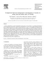
Comparision between background concentration of arsenic in urban and non urban areas of florida

Advances in Environmental Research 8 (2003) 137–146
1093-0191/03/$ - see front matter ᮊ 2003 Elsevier Science Ltd. All rights reserved.
doi:10.1016/S1093-0191(02)00138-7
Comparison between background concentrations of arsenic in
urban and non-urban areas of Florida
Tait Chirenje *, Lena Q. Ma , Ming Chen , Edward J. Zillioux
a, aa b
Soil and Water Science Department, University of Florida, Gainesville, FL 32611, USA
a
Florida Power and Light, 700 Universe Boulevard, Juno Beach, FL 33408, USA
b
Received 10 April 2002; received in revised form 5 November 2002; accepted 17 November 2002
Abstract
Arsenic contamination is of great environmental concern due to its toxic effects as a carcinogen. Knowledge of
arsenic background concentrations is important for land application of wastes and for making remediation decisions.
The soil clean-up target level for arsenic in Florida (0.8 and 3.7 mg kg for residential and commercial areas,
y1
respectively) lies within the range of both background and analytical quantification limits. The objective of this study
was to compare arsenic distribution in urban and non-urban areas of Florida. Approximately 440 urban and 448 non-
urban Florida soil samples were compared. For urban areas, soil samples were collected from three land-use classes
(residential, commercial and public land) in two cities, Gainesville and Miami. For the non-urban areas, samples
were collected from relatively undisturbed non-inhabited areas. Arsenic concentrations varied greatly in Gainesville,
ranging from 0.21 to approximately 660 mg kg with a geometric mean (GM) of 0.40 mg kg , which were lower
y1 y1
than Miami samples (ranging from 0.32 to 112 mg kg ; GMs2.81 mg kg ). Arsenic background concentrations
y1 y1
in urban soils were significantly greater and showed greater variation than those from relatively undisturbed non-
urban soils (GMs0.27 mg kg ) in general.
y1
ᮊ 2003 Elsevier Science Ltd. All rights reserved.
Keywords: Background concentration; Natural and anthropogenic; Arsenic; Florida

1. Introduction
Arsenic occurs naturally in a wide range of minerals
in soils. This, coupled with the once widespread use of
arsenic pigments, insecticides, herbicides, and industrial
wastes, makes it a common trace constituent of most
soils. In fact, arsenic is the 20th most abundant element
Abbreviations: AM, arithmetic mean; ASD, arithmetic
standard deviation; CEC, cation exchange capacity; FCSSP,
the Florida Cooperative Soil Survey Program; GM, geometric
mean; GSD, geometric standard deviation; OC, organic carbon;
SCTL, soil clean-up target level.
*Corresponding author. Tel.: q1-352-392-1951; fax: q1-
352-392-3902.
E-mail address: (T. Chirenje).
in the earth’s crust and is a major constituent of )245
different minerals with sulfur deposits being the most
common culprits (Woolson, 1983). Arsenic concentra-
tions are variable even in virgin components of the
environment including soils, sediments, bodies of water,
animals, and plants.
Since arsenic is a known human carcinogen, its
distribution and behavior in soils needs to be docu-
mented to better understand its human exposure. The
United States Environmental Protection Agency (USE-
PA) has set the levels of arsenic allowed in oral intake,
drinking water and breathing air at 0.0003
mg kg d , 0.050 mg l and 0.0043 mg m , respec-
y1 y1 y1 y3
tively, (USEPA, 1998). The World Health Organization
(WHO) has, in fact, recommended lowering the primary

drinking water standard to 0.010 mg l .
y1
138 T. Chirenje et al. / Advances in Environmental Research 8 (2003) 137–146
Arsenic was widely used in Florida during the early
part of the 20th century as an insecticide to control
disease-carrying ticks on cattle. Arsenic was also used,
along with copper and chromium as a wood preservative
(CCA, Grant and Dobbs, 1977). The most common
present day uses of arsenic compounds include pesti-
cides, wood preservatives and as growth promoters for
poultry and pigs (O’Neill, 1990). Mining activities,
smelters and fuel combustion also contribute significant
amounts of arsenic to the environment.
Arsenic distribution in Florida soils is likely to
encompass at least three populations of concentrations,
which may or may not be easily distinguishable. These
include (1) natural background, (2) a diffuse anthro-
pogenic influence, or ‘anthropogenic background,’ and
(3) localized point sources. The relative proportion of
each population varies between urban and non-urban
areas. Therefore, knowing the distribution of arsenic in
these three populations in both urban and non-urban
soils aids our understanding of the impacts of human
activity on natural concentrations of arsenic in soils
(O’Neill, 1990).
Significant land-use changes have occurred over the
decades due to the migration of people to Florida in
search of warmer climate and better economic oppor-
tunities. Currently, 11% of the total land area in Florida
(total area 14 258 000 ha) is considered urbanized

(Nizeyimana et al., 2001) and this urbanization trend
continues to increase. This is relatively greater than the
national urbanized area of 3%.
Unlike natural areas, arsenic concentrations in urban
soils vary considerably over short intervals. Urban soils
are complex and heterogeneous in their structure and
composition (Craul, 1985; Davies et al., 1987). Human
activity is the predominant active agent in the modifi-
cation of these soils (Barrett, 1987). A fitting definition
of an urban soil is, a soil material having a non-
agricultural, usually manmade surface layer more than
50 cm thick, that has been produced by mixing or
filling of the land surface in urban and suburban areas
(Craul, 1985). There is a greater probability of historic
anthropogenic contamination, vertical mixing during
development, use of fill from different geologic areas,
deposition andyor contributions from the use of pesti-
cides or amendments from other sources in urban areas
than non-urban areas (Craul, 1985; Thornton, 1987).
Intensive human activity significantly alters the original
native soils, making it difficult to describe urban soils
using typical soil classification schemes.
Arsenic concentrations in relatively undisturbed areas
can still be attributed to purely geological factors with
a few exceptions where non-point sources due to agri-
cultural use of arsenic-containing pesticidesyherbicides
and aerial deposition are significant. It may still be
reasonable to consider the arsenic concentrations in
these soils as the true natural arsenic background con-
centrations. Areas that have had significant human

activity (urban soils in general) are likely to exhibit
what we may call ‘anthropogenic background concen-
trations’ of arsenic.
Background concentrations of arsenic in relatively
undisturbed Florida soils are established and they vary
from 0.01 to 61.1 mg kg , with a geometric mean
y1
(GM) of 0.27 mg kg (Chen et al., 1999). Typical soil
y1
arsenic concentrations range between 0.1 and 40
mg kg worldwide, with an arithmetic mean (AM)
y1
concentration of 5–6 mg kg (Kabata-Pendias and
y1
Pendias, 1992). A survey of soils in the US indicated
that arsenic levels for undisturbed soils ranged from
-0.1 to 97 mg kg with a GM arsenic concentration
y1
of 5.2 mg kg (Shacklette and Boerngen, 1984).
y1
This investigation was conducted to (i) compare
arsenic background concentrations in urban and non-
urban soils in Florida, and (ii) investigate the relation-
ship between arsenic background concentrations and the
extent of human activity and other soil properties. A
medium-sized city (Gainesville) and a relatively large
city (Miami, in terms of population and level of devel-
opment) were used to represent urban areas.
2. Methodology
Three different sets of samples (i) urban soils col-

lected from a medium-sized city, Gainesville (popula-
tion, 96 000; size, 93 km ), (ii) urban soils collected
2
from a relatively large city, Miami (population, 370 000;
size, 91 km ), and (iii) natural soils from relatively
2
undisturbed non-urban soils, were used.
2.1. Soils from undisturbed areas
The non-urban soils used in this study were sampled
and characterized as a part of the Florida Cooperative
Soil Survey Program conducted jointly by the University
of Florida Soil and Water Science Department and the
United States Department of Agriculture–Natural
Resources Conservation Service (USDA–NRCS). Dur-
ing sampling, great care was taken to select sites without
known sources of anthropogenic contamination. Soil
horizons were delineated and sampled using USDA
guidelines (Soil Survey Division Staff, 1993). Based on
the mean coefficient of variation from a previous study
(Ma et al., 1997), a minimum of 214 soil samples were
required to establish a statistically valid database for
Florida soils (with 95% confidence level and 20%
accepted variability between samples). However, a total
of 448 archived soil samples were selected to assure
both taxonomic and geographic representation.
The overall taxonomic representation was achieved
by weighting the number of samples for each soil order
by their estimated areal occurrences in Florida. The
total mapped area was 11 265 530 ha and covered
139T. Chirenje et al. / Advances in Environmental Research 8 (2003) 137–146

approximately 80% of Florida’s total land area. Seven
soil orders were identified from 51 to 67 counties and
their approximate coverage was: Spodosols (28%), Enti-
sols (22%), Ultisols (19%), Alfisols (14%), Histosols
(10%), Mollisols (4%), and Inceptisols (3%). Based on
the areal occurrence of each soil order, the samples
included surface horizons from 122 Spodosols, 107
Entisols, 90 Ultisols, 60 Alfisols, 39 Histosols, 17
Mollisols, and 13 Inceptisols.
2.2. Soils from urban areas (Gainesville and Miami)
The Gainesville study was done as a pilot test to
develop a comprehensive sampling protocol for other
cities. The number of samples collected was based on
soil heterogeneity and determined using the following
Eq. (1):
2
wz
x|
Ns S=t yR (1)
Ž.
a
y~
where N is the number of samples, S is the estimated
standard deviation of the AM of all single values (in
this case, S was calculated from the 25 samples collected
from the University of Florida campus in Gainesville),
t is the Student t value for a given confidence interval
a
(1.96 for the 95% confidence interval) and R is the
accepted variability in mean estimation (usually 10–

20% depending on the scale and budget of project).A
value of 20% was used and the minimum number of
samples needed for Gainesville was determined to be
130.
Three land-uses were selected for sampling. These
were residential, commercial and public land. These
were chosen because they cover the largest area in most
urban settings. Differentiating the samples from these
three land-use classes enabled us to test for differences
among them. The number of categories selected from
these three land-uses depends on the depth of detail
required in the final sample.
Five categories were chosen from the three land-uses
in Gainesville (i.e. residential right-of-way, residential
yards, public buildings, public parks and commercial
areas). Forty surface samples (0–20 cm depth) were
collected in May 2000 from each category, resulting in
a total of 200 samples. One out of every 5 samples
taken from each category was duplicated (for compari-
son of reproducibility), bringing the total number of
samples to 240. However, at least three cores were
taken and composited at each of the remaining sites.
The sites for sample collection were randomly selected
within each category of land-use using a set of strict
exclusion criteria to avoid any potentially contaminated
areas. Chirenje et al. (2001) discuss both the randomi-
zation process and the exclusion criteria in detail.
Based on the pilot study, no significant difference
was observed in arsenic concentrations between soils in
residential-yard and residential-right-of-way, thus the

latter was used to represent residential soil, reducing
land-use categories to four for all subsequent studies. It
was also later determined that the focus of such back-
ground studies should produce a good estimate of the
overall concentration distribution in each stratum with-
out primarily focusing on the central tendency of each
stratum. Therefore the precision target would be set on
an upper percentile of the concentration distribution.
Conover (1980) described a method for calculating the
minimum number of samples needed for a given per-
centile of a distribution to be exceeded by the maximum
observed sample value with a given confidence level.
For example, the sample size needed to assure exceed-
ence of the upper 95th percentile with 95% confidence
is 59. Based on this, 60 samples (0–10 cm depth) were
collected in January, 2001 from four land-use categories
in the Miami study (residential areas, commercial areas,
public parks and public buildings). The change in depth
was instituted after the revision of the sampling protocol
and depths of 0–10, 10–30 and 30–60 cm were subse-
quently sampled in Miami and other cities that followed.
However, results from the top 10 cm only are discussed
in this publication. These changes are discussed in detail
by Chirenje et al. (2001).
2.3. Sample preparation and trace element analysis
All soil samples were air dried, ground, and passed
through a 2-mm sieve. The screened samples were
stored in sealed polyethylene containers before analysis.
The non-urban soils were digested using USEPA Meth-
od 3051a whereas for the urban soils, USEPA Method

3051 was used. A simpler protocol, USEPA Method
3051, was instituted after the non-urban soils study,
therefore the new method was used for the urban soils
study. The soils were digested in a microwave digester
using USEPA Method 3051 (or 3051a), which is com-
parable to USEPA Method 3050, the hotplate digestion
method (USEPA, 1996). In summary, 0.5–2 g of soil
samples were weighed into 120-ml Teflon tubes and
digested in 9 ml of concentrated HNO for Method
3
3051 (or 9 ml of concentrated HNO plus 3 ml of
3
concentrated HCl for Method 3051a) in a CEM MDS-
2000 microwave digester (Matthews, NC). For Histo-
sols rich in organic matter, only 0.5 g of sample was
used and 1.0 ml of H O was added prior to digestion.
22
The resulting solution was filtered through a Whatman
No. 42 filter paper and made up to 100 ml. Arsenic
concentrations in the digests (or digested samples) were
determined on a SIMAA 6000 graphite furnace atomic
absorption spectrophotometer (GFAAS, Perkin-Elmer,
Norwalk, CT) using USEPA method 7060A (USEPA,
1995).
140 T. Chirenje et al. / Advances in Environmental Research 8 (2003) 137–146
Table 1
Summary statistics for soil arsenic concentrations in different land-uses in Gainesville and Miami (all concentrations in mg kg )
y1
Urban soils Non-urban soils
Residential Commercial Public parks Public buildings Combined South Florida

c
North Florida
c
Miami
࠻ of samples 58 60 60 59 237 65 158
AM
a
5.37 2.56 0.52 3.46 4.00 2.71 0.85
Median 3.47 2.11 3.29 2.39 2.60 0.24 0.20
GM
b
3.72 1.93 3.49 2.49 2.80 0.44 0.21
GSD
b
2.25 1.99 2.13 2.24 2.24 7.37 4.09
Gainesville
࠻ of samples 79 39 38 40 196 65 158
AM 0.68 1.19 0.52 0.57 0.73 2.71 0.85
Median 0.52 0.52 0.35 0.48 0.50 0.24 0.20
GM 0.46 0.63 0.23 0.34 0.40 0.44 0.21
GSD
b
2.27 0.88 2.58 1.33 1.57 7.37 4.09
AM, arithmetic mean.
a
GM, geometric mean; GSD, geometric standard deviation.
b
South Florida includes Miami and North Florida includes Gainesville.
c
In addition, soil properties that have been shown to

affect arsenic concentrations (pH, clay content, total
organic carbon (OC), and total Fe and Al) were meas-
ured using internationally accepted standard procedures
(Page et al., 1982). The concentrations of Fe and Al
were determined using a Thermo-Jerroll Ash 61E Induc-
tively Coupled Plasma Atomic Emission Spectropho-
tometer (ICP-AES, Spectro, Fitchburg, MA).
2.4. Data analyses
All element concentrations are presented on a dry
matter basis. Both AM and GM were used to describe
the central tendency of the data. Baseline concentrations
of arsenic were calculated using GMyGSD and
2
GM=GSD (upper baseline limit (UBL)) of the sam-
2
ples, which include 97.5% of the sample population
(Dudka et al., 1995). Chen et al. (1999) provide details
on definition and calculation of baseline concentrations.
All statistical analyses were performed using SAS
᭨
(SAS Institute, 2000). The generalized linear model
was used in preference to the analysis of variance
procedure to account for the unequal number of samples
within each class and quantile–quantile (QQ) plots were
used to eliminate outliers from our dataset. These
outliers represented samples with abnormally high
arsenic concentrations that could not be attributed to the
background levels. However, outliers were not eliminat-
ed when distribution graphs were plotted. The Shapiro-
Wilks test was used to test for normality. Because the

distribution of arsenic concentrations was not normal
(data not shown), the data were log-transformed before
analysis to meet the assumption of normality required
for the regression model.
Spatial analyses were done using Spatial Analyst
tools in Arcview Geographical Information Systems
᭨
software (ESRI, Redlands, CA). Pathfinder (Trimble,
᭨
Sunnyvale, CA) was used to geoprocess the Global
Positioning System unit-logged positions and transform
them into forms that could be read by Arcview . These
᭨
images were used to assess spatial distribution, and
graphically display the analytical results from the study
on a digital map (not shown).
3. Results and discussion
It is important to note that most Florida soils are very
sandy. This leads to low retention of trace elements in
general, with important implications on regulatory con-
centrations for many trace elements. Furthermore, the
populations in this study only approached the normal
distribution after log-transformation. Therefore, the 95%
upper confidence limit (UCL) of the mean was calcu-
lated using the H-statistic from Eq. (2):
22 0.5
wx
UCL sexp(x q0.5s qs =H y ny1 )(2)
1ya y1ya
where x is the AM of the log-transformed data, s is

y
the standard deviation of the log-transformed data, n is
the number of samples, H and H are the H-statistic
1yaa
from tables provided by Land (1975) for the UCL. The
UCL depends on x , n and the chosen confidence limit
y
(Gilbert, 1987). Therefore, the calculated UBL, dis-
cussed previously, was also based on the GM.
3.1. Comparison of soil arsenic concentrations between
urban and non-urban areas
Table 1 summarizes the mean concentrations and
other relevant descriptive statistics for soil arsenic con-
141T. Chirenje et al. / Advances in Environmental Research 8 (2003) 137–146
Fig. 1. Soil arsenic concentration (raw data) distribution in (a)
Gainesville (ns200), (b) Miami (ns240), and non-urban
areas (ns448) in Florida.
Table 2
The UCL, 95th percentile and percentage of soil samples with arsenic concentrations exceeding the SCTL (residential and com-
mercial) in different areas in Florida
Gainesville North Florida Miami South Florida
AM 0.73 0.85 4.00 2.71
UCL
a
as0.05
0.99 2.14 4.30 11.6
UBL
b
as0.05
2.30 3.32 14.3 22.1

%)0.8 (mg kg )
c y1
29.4 16.5 94.6 43.8
%)3.7 (mg kg )
d y1
4.00 5.06 32.5 14.1
UCL : upper confidence limit of the mean at as0.05.
a
as0.05
UBL : upper baseline limit at as0.05.
b
as0.05
0.8 mg kg : the Florida SCTL for residential areas.
c y1
3.7 mg kg : the Florida SCTL for commercial areas.
d y1
centrations in non-urban areas surrounding the two cities
and land-use categories analyzed within the two urban
areas. The distributions of arsenic concentrations in the
three separate classes, with the exception of values
greater than 60 mg kg , are shown in Fig. 1. For the
y1
non-urban soils, samples from South Florida (ns65)
and North Florida (ns158) were used to compare with
Miami and Gainesville samples, respectively. Arsenic
concentrations from the urban areas of Miami and
Gainesville were significantly greater than those from
non-urban soils (as0.05) in the same regions
(GM s0.44 vs. GM s2.80 and
South Florida Miami

GM s0.21 vs. GM s0.40 mg kg ;
y1
North Florida Gainesville
Table 1). As discussed earlier, non-urban soils have
lesser anthropogenic disturbances than urban areas as
they are not exposed to the same activities that often
lead to increases in concentrations of trace elements in
urban soils. In general, the differences in the distribution
of arsenic in urban areas can be attributed to land-use,
while those in non-urban areas can be attributed to soil
forming factors.
Based on the GM, the upper baseline limit
(UBL , 95% of all data fall below this value) and
as0.05
the 95% upper confidence level (UCL) of the GM for
both urban and non-urban soils were calculated (Table
2). The combined UBL for all the land-use cate-
as0.05
gories for Miami (14.3 mg kg ) was more than 6
y1
times greater than for Gainesville (2.3 mg kg ; Table
y1
2). Both the UCL and UBL are dependent on the
variation of the data set, hence these results demonstrate
the greater variation in urban areas than non-urban
areas. The UCL is not a very reliable measure of the
confidence level of the mean for background studies
because it is highly dependent on the number of sam-
ples, approaching the mean as the number of samples
increases. Table 1 demonstrates this point for both

Gainesville and Miami. The UCL is generally useful
for site-specific measurements of arsenic concentrations.
Comparison of properties of soils from Gainesville
with soils collected from non-urban areas close to the
city and on the same parent material did not show any
significant difference, except for pH. This is discussed
in more detail in a later section. There was a significant
difference between urban soils from Miami and non-
urban soils from the surrounding areas. The non-urban
areas surrounding Miami had significantly greater arsen-
142 T. Chirenje et al. / Advances in Environmental Research 8 (2003) 137–146
Table 3
Comparison of pH, OC and siltqclay content between urban
and non-urban soils
Non-urban Gainesville Miami
pH 5.04 6.31 7.23
Siltqclay (%)
a
10.6 9.30 28.0
OC (%)
b
4.50 1.40 5.70
Siltqclay: represents the sum of silt and clay as a
a
percentage.
Organic carbon.
b
ic background concentrations than both the non-urban
and urban areas in Gainesville (Fig. 1; Table 1). These
differences can be attributed to the different soils, which

are a manifestation of different parent materials in these
two regions. The comparison between public parks in
each city and non-urban soils in areas surrounding the
same city provided the best results because public parks
in most urban areas have very little human disturbance.
However, it must be noted that most of the parks in
Miami had significant fill in them, unlike parks in
Gainesville.
Another comparison was also made between ‘dis-
turbed’ and ‘undisturbed’ non-urban soils, where dis-
turbed soils represented areas that had significant
anthropogenic influence e.g. farmland, managed plan-
tations etc. There was no significant difference between
undisturbed and disturbed non-urban soils (GMs0.25
and 0.29 mg kg , respectively). This can be explained
y1
by the fact that, although disturbed non-urban soils have
some anthropogenic influence, these activities do not
directly lead to contamination by point sources, as is
the case in most urban areas.
There were significant interactions between cities and
land-use categories, hence comparisons of the combined
land-use categories from the two cities from non-urban
areas were not possible. Nonetheless, all four land-use
classes in Miami had significantly greater arsenic con-
centrations than the corresponding land-use classes in
Gainesville (Table 1). In fact, the land-use category
with the lowest arsenic concentration in Miami (public
parks) had significantly greater arsenic concentrations
than the land-use category with the highest arsenic

concentration in Gainesville (commercial areas).
Approximately a third of all samples collected in Miami
had arsenic concentrations greater than the Florida soil
clean-up target level (SCTL) for commercial areas, 3.7
mg kg . Gainesville, on the other hand, had approxi-
y1
mately 29% samples above the Florida SCTL for resi-
dential areas and only 4% were above the SCTL of 3.7
mg kg for commercial areas. Corresponding propor-
y1
tions of samples falling above the SCTL for residential
and commercial areas in both North and South Florida
non-urban areas were lower than those of Gainesville
and Miami, respectively (with the notable exception of
North Florida for the commercial SCTL, Table 2).
The differences in the arsenic concentrations between
Gainesville and Miami soils can be explained by several
factors. First, the depth of sampling for the top layer of
soil was different between the two cities. The sampling
depth for the analyzed samples in Gainesville was 0–
20 cm while that in Miami was 0–10 cm. This has
important implications on the observed concentrations
because arsenic concentrations generally decrease with
depth in the top 30 cm of soil. However, we can still
compare results from these two cities because a smaller
subsample (ns30) that was reanalyzed in Miami
showed a difference in arsenic concentration of less
than 30% between 0–10 and 10–20 cm depths. This
difference is relatively smaller in magnitude than the
difference between the two cities (Gainesville and

Miami). Comparisons of arsenic concentrations between
the depths of 0–10 and 10–20 cm in Daytona Beach
(ns64) also showed very small differences, possibly
due the to the extensive mixing in the top 50 cm in
urban soils (data not shown). Secondly, Gainesville
soils have greater sand (quartz) content than Miami
soils (91 vs. 72%, Table 3) which is expected to
facilitate greater arsenic leaching or loss with runoff.
The presence of significant amounts of carbonate in
South Florida soils, 30–94% CaCO (Li, 2001) would
3
also help retain trace elements and hence such soils are
expected to show greater accumulation of anthropogen-
ically-added trace elements such as arsenic.
The high background concentrations of soil arsenic
observed in the urban areas in Florida are supported by
observations in studies from other parts of the US and
in other countries (Murphy and Aucott, 1998; Tiller,
1992; Tripathi et al., 1997). For example, Folkes and
Kuehster (2001) observed very high baseline concentra-
tions of arsenic in the suburban areas of Denver,
Colorado (residential areas had GM ;6 mg kg while
y1
urban areas in general had GM ;7mgkg ). However,
y1
the rural background concentrations of arsenic in Colo-
rado were also significantly greater than those of Florida
soils (GMs3.7 vs. 0.4 mg kg , respectively). This
y1
difference may be attributed to geologic factors, e.g.

Colorado soils are derived from parent materials with
higher concentrations of arsenic than parent materials
from which Florida soils are derived.
In New Jersey, Murphy and Aucott (1998) attributed
the high arsenic concentrations in residential areas to
historical land-use and former heavily sprayed orchards.
The importance of historical land-use was also demon-
strated by Tiller (1992) in a similar background study
in Australian urban areas. Tiller (1992) avoided areas
whose historical land-uses increase their probability of
being contaminated. In spite of these efforts, arsenic
concentration ranges of -1–8 mg kg were observed.
y1
The relative contributions of both natural and anthro-
143T. Chirenje et al. / Advances in Environmental Research 8 (2003) 137–146
Fig. 2. QQ plots for (a) Gainesville (ns200), (b) Miami (ns
240), and (c) non-urban areas (ns448), for transformed data.
pogenic activities in the distributions of soil arsenic
concentrations were investigated in detail by Bak et al.
(1997). Not surprisingly, they concluded that sludge
application contributed the greatest amount of arsenic
to the soil annually. This has important ramifications
because land spreading of sludge is a common practice
in many urban areas worldwide, and the regulations
governing these applications often have loopholes that
can be exploited by many unscrupulous waste managers.
3.2. Soil arsenic distribution characteristics
The complexity of urban soils often leads to distinct
patterns in arsenic distribution. The distinction between
natural background, anthropogenic background, and

contaminated arsenic concentrations is more discernible
in urban areas than in non-urban areas (Fig. 2). There
is a greater possibility of finding contaminated areas in
urban environments due to greater human disturbance
than in non-urban areas (Fig. 2a). On the other hand,
non-urban areas are likely to exhibit mostly natural
background concentrations of trace elements.
The most critical shortcoming of these distribution
plots is that not all soils that have high concentrations
of arsenic have been exposed to contamination. Some
soils naturally have high arsenic concentrations from
their parent material. The determination of pollution can
only be done if the parent material is known or if the
historical land-use of the sites in question suggests
contamination. Furthermore, some sites with sandy soils
(e.g. most Gainesville sites) may be exposed to contam-
ination, but the arsenic is not retained in the soil long
enough to be picked up in studies like the current one.
In such cases, the low concentration observed is not
necessarily the natural background. Such a determina-
tion can only be made if the groundwater at all sites is
analyzed. However, analyzing groundwater may not
provide the clues needed if enough time elapses between
the pollution and sampling events.
Censoring data on both ends (non-detects and outli-
ers) can also have a significant impact on the shape and
nature of the distributions. The plots of the Gainesville
data demonstrate this point. Lower end censoring (non-
detects) may yield a set of ‘equal’ concentrations
leading to clumping on the lower (left tail) end of the

curve. Furthermore, if the data are also censored at the
high end before plotting the distributions, the ‘contam-
inated sites’ disappear from the distribution. Nonethe-
less, the slope of the curves gives us a clear indication
of the variation in each sample stratum.
3.3. Correlation between soil arsenic concentrations
with soil properties
Correlation is widely used in trace element analyses
(Bradford et al., 1996; Dudka et al., 1995; Lee et al.,
1997) because of its ability to quantify how one factor
changes in response to the other. Correlation analyses
between elemental concentrations and soil properties
(total Fe, total Al, pH, clay, OC, and cation exchange
capacity (CEC)) of both the urban and non-urban soils
were conducted in this study. The correlation between
pH and arsenic concentrations in urban areas was both
very low statistically insignificant.
There was higher correlation between clay content
and arsenic concentration in the non-urban soils than
urban soils (Table 4, significant at as0.05). This is
consistent with previously published data by Ma et al.
(1997). They reported that arsenic concentrations were
strongly correlated with clay content in 40 Florida
surface soils. Higher correlation was also reported
between clay content and concentrations of arsenic in
Canadian (Mermut et al., 1996), Polish (Dudka, 1993)
and Dutch soils (Forstner, 1995; Edelman and de Bruin,
1986) suggesting that clay content is important in
controlling the level and distribution of trace metal
concentrations in soils. A study conducted in both urban

and non-urban areas in Denmark and Holland showed
144 T. Chirenje et al. / Advances in Environmental Research 8 (2003) 137–146
Table 4
Correlation coefficients of arsenic concentrations with soil
a
properties in urban and non-urban areas
Element pH Clay OC Total Fe Total Al
Non-urban 0.14 0.33* 0.58* 0.66* 0.60*
Gainesville 0.10 0.01 y0.05 y0.04 0.02
Miami 0.09 0.04 y0.08 -0.09 y0.06
Correlations coefficients denoted with ‘*’ are significant at
a
as0.05.
low correlation coefficients for soil texture although
clay soils consistently had higher arsenic concentration
than sandy soils in the non-urban areas (Bak et al.,
1997). The investigation concluded that arsenic concen-
trations in studied areas were more sensitive to soil
factors (e.g. clay content) than anthropogenic activities.
Anthropogenic activities in urban areas, especially the
use of fill, tend to interfere with the relationship between
soil forming factors and trace element concentrations.
In contrast to urban soils, there was significant cor-
relation between OC and arsenic concentrations in non-
urban areas (Table 4). Humic substances in organic
soils (peat) can serve as strong reducing and complexing
agents and influence the processes controlling mobili-
zation of many toxic elements including arsenic (Gough
et al., 1996). Similar to the results from the non-urban
soils, other researchers have reported strong positive

correlation between trace element concentrations and
OC and the siltqclay content of the soil (Aloupi and
Angelidis, 2001; Chirenje, 2000; Wilcke et al., 1998).
There was significant (as0.05) correlation between
arsenic concentrations and total Fe and Al concentra-
tions in non-urban soils (Table 4). Both Fe and Al react
with the arsenate to form stable, immobile compounds
in the soil, and oxides and hydroxides of both elements
also provide reactive surfaces on which arsenic can be
adsorbed. However, the same trend was not observed in
urban soils, possibly due to the increased use of fill.
Dudka (1993) found good correlation between concen-
trations of arsenic and concentrations of Al and Fe in
surface soils of Poland. He concluded that levels of
most elements were mainly controlled by the minerals
(Fe and Al oxides) present in the soils (Dudka, 1992).
Total Fe and Al concentrations (2300 and 2200
mg kg ) in Florida soil are 16–32 times lower than
y1
the average concentrations reported for other soils
(38 000 and 71 000 mg kg ; Lindsay, 1979). Nonethe-
y1
less, total Fe and Al, even at such low concentrations,
are significant in controlling metal concentrations in
Florida soils.
Multiple regression of concentrations of trace elemen-
ts against clay, OC, pH, CEC, and total concentrations
of Al and Fe supported the relationships of trace
elements with important soil properties (data not
shown). Regressions of log-transformed concentrations

of arsenic against six soil variables explained between
9 and 65% of the total variance. However, no such
correlation was observed in urban areas. In the non-
urban soils, partial correlation analyses confirmed that
total Fe and total Al were the two major variables
controlling concentrations and distributions of arsenic
in Florida surface soils as demonstrated previously using
simple correlation analysis.
4. Conclusions
This study compared the distribution of arsenic in
soils from urban and non-urban areas. In general, arsenic
concentrations in urban areas were higher than those in
non-urban areas. Arsenic concentrations varied signifi-
cantly with land-use in Miami but only parks had lower
arsenic concentration than the other land-uses in Gaines-
ville. Soil arsenic concentrations in non-urban areas
showed significant correlation with natural soil proper-
ties (clay content, OC, and total Fe and Al) because
they are exposed to relatively lower disturbance than
urban soils. Knowledge of classical pedology can easily
be employed to predict arsenic distribution in these
areas. On the other hand, land-use categories can serve
as good indicators of arsenic distribution in urban areas.
More research is needed to better understand the tem-
poral variation of arsenic in different compartments in
both urban and non-urban areas so that better decisions
can be made about land application of waste and
remediation of possibly contaminated soils.
Acknowledgments
This research was sponsored in part by the Florida

Center for Solid and Hazardous Waste Management
(Contract No. 96011017) and Florida Power and Light.
Helpful discussions and consultations with Dr John
Thomas of the Soil and Water Science Department at
the University of Florida, and Drs Patricia Cline (Golder
Associates) and Thomas Potter (USDA) are gratefully
acknowledged. The authors would also like to thank Dr
Peter Hooda for his help in improving the manuscript
after initial review.
References
Aloupi, M., Angelidis, M.O., 2001. Geochemistry of natural
and anthropogenic metals in the coastal sediments of the
island of Lesvos, Aegean Sea. Environ. Pollut. 133,
211–219.
Bak, J., Jensen, J., Larsen, M.M., Pritz, G., Scott-Fordsmand,
J., 1997. A heavy metal monitoring programme in Denmark.
Sci. Total Environ. 207, 179–186.
145T. Chirenje et al. / Advances in Environmental Research 8 (2003) 137–146
Barrett, I., 1987. Research in Urban Ecology. Report to the
Nature Conservancy Council.
Bradford, G.R., Chang, A.C., Page, A.L., 1996. Background
concentrations of trace and major elements in California
soils. Kearney Foundation Special Report, University of
California, Riverside, March 1996, pp. 1–52.
Chen, M., Ma, L.Q., Hornsby, A.G., Harris, W.G., 1999.
Background concentrations of trace metals in Florida surface
soils: taxonomic and geographic distributions of total–total
and total recoverable concentrations of selected trace metals.
Florida Center for Solid and Hazardous Waste Management.
Report 99–7.

Chirenje, T., 2000. Chemical and physical changes in a wood
ash-amended forest soil. Ph.D. Dissertation, University of
Florida, Gainesville, Florida.
Chirenje, T., Ma, L.Q., Harris, W.G., Hornsby, H.G., Zillioux,
E.Z., Latimer, S., 2001. Protocol development for assessing
arsenic background concentrations in urban areas. Environ.
Forensics 2, 141–153.
Conover, W.J., 1980. Practical Nonparametric Statistics. Wiley,
New York.
Craul, P.J., 1985. A description of urban soils and their desired
characteristics. J. Arboric. 11, 330–339.
Davies, D.J.A., Watt, J.M., Thornton, I., 1987. Lead levels in
Birmingham dusts and soils. Sci. Total Environ. 67,
177–185.
Dudka, S., 1992. Factor analysis of total element concentra-
tions in surface soils of Poland. Sci. Total Environ. 121,
39–52.
Dudka, S., 1993. Baseline concentrations of As, Co, Cr, Cu,
Ga, Mn, Ni and Se in surface soils, Poland. Appl. Geochem.
2, 23–28.
Dudka, S., Ponce-Hernandez, R., Hutchinson, T.C., 1995.
Current levels of total element concentrations in the surface
layer of Sudbury’s soils. Sci. Total Environ. 162, 161–172.
Edelman, T., de Bruin, M., 1986. Background values of 32
elements in Dutch topsoils, determined with non-destructive
neutron activation analysis. In: Assink, J.W., van den Brink,
J. (Eds.), Contaminated Soil. Martinus Nijhoff Publishers,
Dordrecht, pp. 88–98.
Folkes, D.J., Kuehster, T.E., 2001. Contributions of pesticide
use to urban background concentrations of arsenic in Den-

ver, Colorado, USA. Environ. Forensics 2, 127–139.
Forstner, U., 1995. Land contamination by metals: global
scope and magnitude of problem. In: Allen, H.E., Huang,
C.P., Bailey, G.W., Bowers, A.R. (Eds.), Metal Speciation
and Contamination of Soil. Lewis Publishers, Boca Raton,
FL, pp. 1–33.
Gilbert, R.O., 1987. Statistical Methods for Environmental
Pollution Monitoring. Wiley, New York, NY.
Gough, L.P., Kotra, R.K., Holmes, C.W., et al., 1996. Chemical
analysis results for mercury and trace elements in vegetation,
water, and organic-rich sediments, South Florida. USGS
Openfile Report 96-091. Denver Federal Center, Denver,
CO.
Grant, C., Dobbs, A.J., 1977. The growth and metal content
of plants grown in soil contaminated by a copperychromey
arsenic wood preservative. Environ. Pollut. 14, 213–226.
Kabata-Pendias, A., Pendias, H., 1992. Trace Elements in Soils
and Plants. second ed. CRC Press, Boca Raton, FL.
Land, C.E., 1975. Tables of confidence limits for linear
functions of the normal mean and variance. Selected Tables
in Mathematical Statistics, vol. 3. American Statistical Soci-
ety, Providence, RI, pp. 385–419.
Lee, B.D., Carter, B.J., Basta, N.T., Weaver, B., 1997. Factors
influencing heavy metal distribution in six Oklahoma bench-
mark soils. Soil Sci. Soc. Am. J. 61, 218–233.
Li, Y., 2001. Calcareous Soils in Miami-Dade County. Florida
Coop. SL 183. Fla. Coop. Ext. Ser. IFAS, University of
Florida, Gainesville, FL.
Lindsay, W.L. (Ed.), 1979. Chemical Equilibria in Soils.
Wiley, New York.

Ma, L.Q., Tan, F., Harris, W.G., 1997. Concentrations and
distributions of eleven elements in Florida soils. J. Environ.
Qual. 26, 769–775.
Mermut, A.R., Jain, J.C., Song, L., Kerrich, R., Kozak, L.,
Jana, S., 1996. Trace element concentrations of selected
soils and fertilizers in Saskatchewan, Canada. J. Environ.
Qual. 25, 845–853.
Murphy, E.A., Aucott, M., 1998. An assessment of the amounts
of arsenical pesticides used historically in a geographic area.
Sci. Total Environ. 218, 89–101.
Nizeyimana, E.L., Petersen, G.W., Imhoff, M.L., et al., 2001.
Assessing the impact of land conversion to urban use on
soils with different productivity levels in the USA. Soil Sci.
Soc. Am. J. 65, 391–402.
O’Neill, P., 1990. Arsenic. Heavy Metals in Soils. Wiley, New
York, NY, pp. 83–99.
Aravind, P.G., 1982. In: Page, A.L., Miller, R.H., Keeney,
D.R. (Eds.), Methods of Soil Analysis. Part 2-Chemical and
Microbiological Properties. second ed. American Society of
Agronomy, Madison, WI.
SAS Institute, 2000. SAS Users Guide: Statistics. SAS Insti-
tute, Gary, NC.
Shacklette, H.T., Boerngen, J.G., 1984. Element concentrations
in soils and other surficial materials of the conterminous
United States. USGS Professional Paper 1270. US Govt.
Print. Office, Washington, DC.
Soil Survey Division Staff, 1993. Soil Survey Manual. USDA
Handbook No. 18. US Govt. Print. Office, Washington, DC.
Thornton, I., 1987. Metal contamination of soils in urban
areas. In: Bullock, P., Gregory, P.J. (Eds.), Soils in the

Urban Environment. Blackwell Scientific Publications, Lon-
don, UK.
Tiller, K.G., 1992. Urban soil contamination in Australia. Aust.
J. Soil Res. 30, 937–957.
Tripathi, R.M., Raghunath, R., Krishnamorthy, T.M., 1997.
Arsenic intake by the adult population in Bombay City. Sci.
Total Environ. 208, 89–95.
US Environmental Protection Agency, 1995. Test Methods for
Evaluating Solid Waste. Vol IA: Laboratory Manual Physi-
calyChemical Methods SW846, third ed. USEPA Office of
Solid Waste and Emergency Response, Washington DC.
US Environmental Protection Agency, 1996. Microwave
Assisted Acid Dissolution of Sediments, Sludges, Soils and
Oils, second ed. USEPA Office of Solid Waste and Emer-
gency Response, Washington DC, June 1996, pp. 1–22.
146 T. Chirenje et al. / Advances in Environmental Research 8 (2003) 137–146
US Environmental Protection Agency, 1998. Integrated Risk
Information System (IRIS). Arsenic, inorganic. CASRN
7440-38-2. April. Cincinnati, OH.
Wilcke, W., Miller, S., Kanchanakool, N., Zech, W., 1998.
Urban soil contamination in Bangkok: heavy metal and
aluminium partitioning in topsoils. Geoderma 86, 211–228.
Woolson, E.A., 1983. Emissions, Cycling, and Effects of
Arsenic in Soil Ecosystems. Biological and Environmental
Effects of Arsenic. Elservier Science Publishers, Fowler, pp.
52–125.