- Trang chủ >>
- Khoa Học Tự Nhiên >>
- Vật lý
Weak gravitational lensing m bartelmann, p schneider
Bạn đang xem bản rút gọn của tài liệu. Xem và tải ngay bản đầy đủ của tài liệu tại đây (1.6 MB, 225 trang )
arXiv:astro-ph/9912508 v1 23 Dec 1999
Weak Gravitational Lensing
Matthias Bartelmann and Peter Schneider
Max-Planck-Institut f
¨
ur Astrophysik, P.O. Box 1523, D–85740 Garching, Germany
Abstract
We review theory and applications of weak gravitational lensing. After summarising
Friedmann-Lemaˆıtre cosmological models, we present the formalism of gravitational lens-
ing and light propagation in arbitrary space-times. We discuss how weak-lensing effects
can be measured. The formalism is then applied to reconstructions of galaxy-cluster mass
distributions, gravitational lensing by large-scale matter distributions, QSO-galaxy corre-
lations induced by weak lensing, lensing of galaxies by galaxies, and weak lensing of the
cosmic microwave background.
Preprint submitted to Elsevier Preprint 12 July 2006
Contents
1 Introduction 5
1.1 Gravitational Light Deflection 5
1.2 Weak Gravitational Lensing 6
1.3 Applications of Gravitational Lensing 8
1.4 Structure of this Review 10
2 Cosmological Background 12
2.1 Friedmann-Lemaˆıtre Cosmological Models 12
2.2 Density Perturbations 24
2.3 Relevant Properties of Lenses and Sources 33
2.4 Correlation Functions, Power Spectra, and their Projections 41
3 Gravitational Light Deflection 45
3.1 Gravitational Lens Theory 45
3.2 Light Propagation in Arbitrary Spacetimes 52
4 Principles of Weak Gravitational Lensing 58
4.1 Introduction 58
4.2 Galaxy Shapes and Sizes, and their Transformation 59
4.3 Local Determination of the Distortion 61
4.4 Magnification Effects 70
4.5 Minimum Lens Strength for its Weak Lensing Detection 74
4.6 Practical Consideration for Measuring Image Shapes 76
5 Weak Lensing by Galaxy Clusters 86
5.1 Introduction 86
5.2 Cluster Mass Reconstruction from Image Distortions 87
2
5.3 Aperture Mass and Multipole Measures 96
5.4 Application to Observed Clusters 101
5.5 Outlook 106
6 Weak Cosmological Lensing 117
6.1 Light Propagation; Choice of Coordinates 118
6.2 Light Deflection 119
6.3 Effective Convergence 122
6.4 Effective-Convergence Power Spectrum 124
6.5 Magnification and Shear 128
6.6 Second-Order Statistical Measures 129
6.7 Higher-Order Statistical Measures 144
6.8 Cosmic Shear and Biasing 148
6.9 Numerical Approach to Cosmic Shear, Cosmological Parameter
Estimates, and Observations 151
7 QSO Magnification Bias and Large-Scale Structure 156
7.1 Introduction 156
7.2 Expected Magnification Bias from Cosmological Density
Perturbations 158
7.3 Theoretical Expectations 162
7.4 Observational Results 167
7.5 Outlook 172
8 Galaxy-Galaxy Lensing 174
8.1 Introduction 174
8.2 The Theory of Galaxy-Galaxy Lensing 175
8.3 Results 178
3
8.4 Galaxy-Galaxy Lensing in Galaxy Clusters 183
9 The Impact of Weak Gravitational Light Deflection on the Microwave
Background Radiation 187
9.1 Introduction 187
9.2 Weak Lensing of the CMB 189
9.3 CMB Temperature Fluctuations 190
9.4 Auto-Correlation Function of the Gravitationally Lensed CMB 190
9.5 Deflection-Angle Variance 194
9.6 Change of CMB Temperature Fluctuations 200
9.7 Discussion 203
10 Summary and Outlook 205
References 211
4
1 Introduction
1.1 Gravitational Light Deflection
Light rays are deflected when they propagate through an inhomogeneous gravita-
tional field. Although several researchers had speculated about such an effect well
before the advent of General Relativity (see Schneider et al. 1992 for a historical
account), it was Einstein’s theory which elevated the deflection of light by masses
from a hypothesis to a firm prediction. Assuming light behaves like a stream of
particles, its deflection can be calculated within Newton’s theory of gravitation, but
General Relativity predicts that the effect is twice as large. A light ray grazing the
surface of the Sun is deflected by 1.75arc seconds compared to the 0.87arc sec-
onds predicted by Newton’s theory. The confirmation of the larger value in 1919
was perhaps the most important step towards accepting General Relativity as the
correct theory of gravity (Eddington 1920).
Cosmic bodies more distant, more massive, or more compact than the Sun can bend
light rays from a single source sufficiently strongly so that multiple light rays can
reach the observer. The observer sees an image in the direction of each ray arriv-
ing at their position, so that the source appears multiply imaged. In the language
of General Relativity, there may exist more than one null geodesic connecting the
world-line of a source with the observation event. Although predicted long before,
the first multiple-image system was discovered only in 1979 (Walsh et al. 1979).
From then on, the field of gravitational lensing developed into one of the most ac-
tive subjects of astrophysical research. Several dozens of multiply-imaged sources
have since been found. Their quantitative analysis provides accurate masses of,
and in some cases detailed information on, the deflectors. An example is shown in
Fig. 1.
Tidal gravitational fields lead to differential deflection of light bundles. The size
and shape of their cross sections are therefore changed. Since photons are neither
emitted nor absorbed in the process of gravitational light deflection, the surface
brightness of lensed sources remains unchanged. Changing the size of the cross
section of a light bundle therefore changes the flux observed from a source. The
different images in multiple-image systems generally have different fluxes. The
images of extended sources, i.e. sources which can observationally be resolved, are
deformed by the gravitational tidal field. Since astronomical sources like galaxies
are not intrinsically circular, this deformation is generally very difficult to identify
in individual images. In some cases, however, the distortion is strong enough to be
readily recognised, most noticeably in the case of Einstein rings (see Fig. 2) and
arcs in galaxy clusters (Fig. 3).
If the light bundles from some sources are distorted so strongly that their images
5
Fig. 1. The gravitational lens system 2237+0305 consists of a nearby spiral galaxy at red-
shift z
d
= 0.039 and four images of a background quasar with redshift z
s
= 1.69. It was
discovered by Huchra et al. (1985). The image was taken by the Hubble Space Telescope
and shows only the innermost region of the lensing galaxy. The central compact source is
the bright galaxy core, the other four compact sources are the quasar images. They differ in
brightness because they are magnified by different amounts. The four images roughly fall
on a circle concentric with the core of the lensing galaxy. The mass inside this circle can be
determined with very high accuracy (Rix et al. 1992). The largest separation between the
images is 1.8
′′
.
appear as giant luminous arcs, one may expect many more sources behind a cluster
whose images are only weakly distorted. Although weak distortions in individual
images can hardly be recognised, the net distortion averaged over an ensemble of
images can still be detected. As we shall describe in Sect. 2.3, deep optical expo-
sures reveal a dense population of faint galaxies on the sky. Most of these galaxies
are at high redshift, thus distant, and their image shapes can be utilised to probe the
tidal gravitational field of intervening mass concentrations. Indeed, the tidal gravi-
tational field can be reconstructed from the coherent distortion apparent in images
of the faint galaxy population, and from that the density profile of intervening clus-
ters of galaxies can be inferred (see Sect. 4).
1.2 Weak Gravitational Lensing
This review deals with weak gravitational lensing. There is no generally applica-
ble definition of weak lensing despite the fact that it constitutes a flourishing area
of research. The common aspect of all studies of weak gravitational lensing is that
measurements of its effects are statistical in nature. While a single multiply-imaged
source provides information on the mass distribution of the deflector, weak lensing
effects show up only across ensembles of sources. One example was given above:
6
Fig. 2. The radio source MG 1131+0456 was discovered by Hewitt et al. (1988) as the
first example of a so-called Einstein ring. If a source and an axially symmetric lens are
co-aligned with the observer, the symmetry of the system permits the formation of a
ring-like image of the source centred on the lens. If the symmetry is broken (as expected for
all realistic lensing matter distributions), the ring is deformed or broken up, typically into
four images (see Fig. 1). However, if the source is sufficiently extended, ring-like images
can be formed even if the symmetry is imperfect. The 6 cm radio map of MG 1131+0456
shows a closed ring, while the ring breaks up at higher frequencies where the source is
smaller. The ring diameter is 2.1
′′
.
The shape distribution of an ensemble of galaxy images is changed close to a mas-
sive galaxy cluster in the foreground, because the cluster’s tidal field polarises the
images. We shall see later that the size distribution of the background galaxy pop-
ulation is also locally changed in the neighbourhood of a massive intervening mass
concentration.
Magnification and distortion effects due to weak lensing can be used to probe the
statistical properties of the matter distribution between us and an ensemble of dis-
tant sources, provided some assumptions on the source properties can be made.
For example, if a standard candle
1
at high redshift is identified, its flux can be
1
The term standard candle is used for any class of astronomical objects whose intrin-
sic luminosity can be inferred independently of the observed flux. In the simplest case, all
members of the class have the same luminosity. More typically, the luminosity depends
on some other known and observable parameters, such that the luminosity can be inferred
from them. The luminosity distance to any standard candle can directly be inferred from the
square root of the ratio of source luminosity and observed flux. Since the luminosity dis-
tance depends on cosmological parameters, the geometry of the Universe can then directly
be investigated. Probably the best current candidates for standard candles are supernovae
of Type Ia. They can be observed to quite high redshifts, and thus be utilised to estimate
7
Fig. 3. The cluster Abell 2218 hosts one of the most impressive collections of arcs. This
HST image of the cluster’s central region shows a pattern of strongly distorted galaxy im-
ages tangentially aligned with respect to the cluster centre, which lies close to the bright
galaxy in the upper part of this image. The frame measures about 80
′′
×160
′′
.
used to estimate the magnification along its line-of-sight. It can be assumed that
the orientation of faint distant galaxies is random. Then, any coherent alignment of
images signals the presence of an intervening tidal gravitational field. As a third ex-
ample, the positions on the sky of cosmic objects at vastly different distances from
us should be mutually independent. A statistical association of foreground objects
with background sources can therefore indicate the magnification caused by the
foreground objects on the background sources.
All these effects are quite subtle, or weak, and many of the current challenges in
the field are observational in nature. A coherent alignment of images of distant
galaxies can be due to an intervening tidal gravitational field, but could also be due
to propagation effects in the Earth’s atmosphere or in the telescope. A variation
in the number density of background sources around a foreground object can be
due to a magnification effect, but could also be due to non-uniform photometry or
obscuration effects. These potential systematic effects have to be controlled at a
level well below the expected weak-lensing effects. We shall return to this essential
point at various places in this review.
1.3 Applications of Gravitational Lensing
Gravitational lensing has developed into a versatile tool for observational cosmol-
ogy. There are two main reasons:
cosmological parameters (e.g. Riess et al. 1998).
8
(1) The deflection angle of a light ray is determined by the gravitational field of
the matter distribution along its path. According to Einstein’s theory of Gen-
eral Relativity, the gravitational field is in turn determined by the stress-energy
tensor of the matter distribution. For the astrophysically most relevant case of
non-relativistic matter, the latter is characterised by the density distribution
alone. Hence, the gravitational field, and thus the deflection angle, depend
neither on the nature of the matter nor on its physical state. Light deflection
probes the total matter density, without distinguishing between ordinary (bary-
onic) matter or dark matter. In contrast to other dynamical methods for probing
gravitational fields, no assumption needs to be made on the dynamical state of
the matter. For example, the interpretation of radial velocity measurements in
terms of the gravitating mass requires the applicability of the virial theorem
(i.e., the physical system is assumed to be in virial equilibrium), or knowledge
of the orbits (such as the circular orbits in disk galaxies). However, as will be
discussed in Sect. 3, lensing measures only the mass distribution projected
along the line-of-sight, and is therefore insensitive to the extent of the mass
distribution along the light rays, as long as this extent is small compared to
the distances from the observer and the source to the deflecting mass. Keeping
this in mind, mass determinations by lensing do not depend on any symmetry
assumptions.
(2) Once the deflection angle as a function of impact parameter is given, gravi-
tational lensing reduces to simple geometry. Since most lens systems involve
sources (and lenses) at moderate or high redshift, lensing can probe the ge-
ometry of the Universe. This was noted by Refsdal (1964), who pointed out
that lensing can be used to determine the Hubble constant and the cosmic
density parameter. Although this turned out later to be more difficult than
anticipated at the time, first measurements of the Hubble constant through
lensing have been obtained with detailed models of the matter distribution
in multiple-image lens systems and the difference in light-travel time along
the different light paths corresponding to different images of the source (e.g.,
Kundi´c et al. 1997; Schechter et al. 1997; Biggs et al. 1998). Since the vol-
ume element per unit redshift interval and unit solid angle also depends on
the geometry of space-time, so does the number of lenses therein. Hence, the
lensing probability for distant sources depends on the cosmological parame-
ters (e.g., Press & Gunn 1973). Unfortunately, in order to derive constraints
on the cosmological model with this method, one needs to know the evolu-
tion of the lens population with redshift. Nevertheless, in some cases, sig-
nificant constraints on the cosmological parameters (Kochanek 1993, 1996;
Maoz & Rix 1993; Bartelmann et al. 1998; Falco et al. 1998), and on the evo-
lution of the lens population (Mao & Kochanek 1994) have been derived from
multiple-image and arc statistics.
The possibility to directly investigate the dark-matter distribution led to sub-
stantial results over recent years. Constraints on the size of the dark-matter
haloes of spiral galaxies were derived (e.g., Brainerd et al. 1996), the pres-
9
ence of dark-matter haloes in elliptical galaxies was demonstrated (e.g.,
Maoz & Rix 1993; Griffiths et al. 1996), and the projected total mass distribution in
many cluster of galaxies was mapped (e.g., Kneib et al. 1996; Hoekstra et al. 1998;
Kaiser et al. 1998). These results directly impact on our understanding of structure
formation, supporting hierarchical structure formation in cold dark matter (CDM)
models. Constraints on the nature of dark matter were also obtained. Compact
dark-matter objects, such as black holes or brown dwarfs, cannot be very abun-
dant in the Universe, because otherwise they would lead to observable lensing ef-
fects (e.g., Schneider 1993; Dalcanton et al. 1994). Galactic microlensing experi-
ments constrained the density and typical mass scale of massive compact halo ob-
jects in our Galaxy (see Paczy´nski 1996, Roulet & Mollerach 1997 and Mao 2000
for reviews). We refer the reader to the reviews by Blandford & Narayan (1992),
Schneider (1996a) and Narayan & Bartelmann (1997) for a detailed account of the
cosmological applications of gravitational lensing.
We shall concentrate almost entirely on weak gravitational lensing here. Hence,
the flourishing fields of multiple-image systems and their interpretation, Galactic
microlensing and its consequences for understanding the nature of dark matter in
the halo of our Galaxy, and the detailed investigations of the mass distribution
in the inner parts of galaxy clusters through arcs, arclets, and multiply imaged
background galaxies, will not be covered in this review. In addition to the refer-
ences given above, we would like to point the reader to Refsdal & Surdej (1994),
Fort & Mellier (1994), and Wu (1996) for more recent reviews on various aspects
of gravitational lensing, to Mellier (1998) for a very recent review on weak lensing,
and to the monograph (Schneider et al. 1992) for a detailed account of the theory
and applications of gravitational lensing.
1.4 Structure of this Review
Many aspects of weak gravitational lensing are intimately related to the cosmo-
logical model and to the theory of structure formation in the Universe. We there-
fore start the review by giving some cosmological background in Sect. 2. After
summarising Friedmann-Lemaˆıtre-Robertson-Walker models, we sketch the the-
ory of structure formation, introduce astrophysical objects like QSOs, galaxies,
and galaxy clusters, and finish the Section with a general discussion of correla-
tion functions, power spectra, and their projections. Gravitational light deflection
in general is the subject of Sect. 3, and the specialisation to weak lensing is de-
scribed in Sect. 4. One of the main aspects there is how weak lensing effects can be
quantified and measured. The following two sections describe the theory of weak
lensing by galaxy clusters (Sect. 5) and cosmological mass distributions (Sect. 6).
Apparent correlations between background QSOs and foreground galaxies due to
the magnification bias caused by large-scale matter distributions are the subject of
Sect. 7. Weak lensing effects of foreground galaxies on background galaxies are
10
reviewed in Sect. 8, and Sect. 9 finally deals with weak lensing of the most distant
and most extended source possible, i.e. the Cosmic Microwave Background. We
present a brief summary and an outlook in Sect. 10.
We use standard astronomical units throughout: 1M
⊙
= 1solar mass = 2×10
33
g;
1Mpc = 1megaparsec = 3.1×10
24
cm.
11
2 Cosmological Background
We review in this section those aspects of the standard cosmological model which
are relevant for our further discussion of weak gravitational lensing. This standard
model consists of a description for the cosmological background which is a homo-
geneous and isotropic solution of the field equations of General Relativity, and a
theory for the formation of structure.
The background model is described by the Robertson-Walker metric
(Robertson 1935; Walker 1935), in which hypersurfaces of constant time are
homogeneous and isotropic three-spaces, either flat or curved, and change with
time according to a scale factor which depends on time only. The dynamics of the
scale factor is determined by two equations which follow from Einstein’s field
equations given the highly symmetric form of the metric.
Current theories of structure formation assume that structure grows via gravita-
tional instability from initial seed perturbations whose origin is yet unclear. Most
common hypotheses lead to the prediction that the statistics of the seed fluctua-
tions is Gaussian. Their amplitude is low for most of their evolution so that lin-
ear perturbation theory is sufficient to describe their growth until late stages. For
general references on the cosmological model and on the theory of structure for-
mation, cf. Weinberg (1972), Misner et al. (1973), Peebles (1980), B¨orner (1988),
Padmanabhan (1993), Peebles (1993), and Peacock (1999).
2.1 Friedmann-Lema
ˆ
ıtre Cosmological Models
2.1.1 Metric
Two postulates are fundamental to the standard cosmological model, which are:
(1) When averaged over sufficiently large scales, there exists a mean motion of
radiation and matter in the Universe with respect to which all averaged ob-
servable properties are isotropic.
(2) All fundamental observers, i.e. imagined observers which follow this mean
motion, experience the same history of the Universe, i.e. the same averaged
observable properties, provided they set their clocks suitably. Such a universe
is called observer-homogeneous.
General Relativity describes space-time as a four-dimensional manifold whose met-
ric tensor g
αβ
is considered as a dynamical field. The dynamics of the metric
is governed by Einstein’s field equations, which relate the Einstein tensor to the
stress-energy tensor of the matter contained in space-time. Two events in space-
time with coordinates differing by dx
α
are separated by ds, with ds
2
= g
αβ
dx
α
dx
β
.
12
The eigentime (proper time) of an observer who travels by ds changes by c
−1
ds.
Greek indices run over 0 3 and Latin indices run over the spatial indices 1 3
only.
The two postulates stated above considerably constrain the admissible form of the
metric tensor. Spatial coordinates which are constant for fundamental observers are
called comoving coordinates. In these coordinates, the mean motion is described by
dx
i
= 0, and hence ds
2
= g
00
dt
2
. If we require that the eigentime of fundamental
observers equal the cosmic time, this implies g
00
= c
2
.
Isotropy requires that clocks can be synchronised such that the space-time compo-
nents of the metric tensor vanish, g
0i
= 0. If this was impossible, the components of
g
0i
identified one particular direction in space-time, violating isotropy. The metric
can therefore be written
ds
2
= c
2
dt
2
+ g
ij
dx
i
dx
j
, (2.1)
where g
ij
is the metric of spatial hypersurfaces. In order not to violate isotropy,
the spatial metric can only isotropically contract or expand with a scale function
a(t) which must be a function of time only, because otherwise the expansion would
be different at different places, violating homogeneity. Hence the metric further
simplifies to
ds
2
= c
2
dt
2
−a
2
(t)dl
2
, (2.2)
where dl is the line element of the homogeneous and isotropic three-space. A spe-
cial case of the metric (2.2) is the Minkowski metric, for which dl is the Euclidian
line element and a(t) is a constant. Homogeneity also implies that all quantities
describing the matter content of the Universe, e.g. density and pressure, can be
functions of time only.
The spatial hypersurfaces whose geometry is described by dl
2
can either be flat or
curved. Isotropy only requires them to be spherically symmetric, i.e. spatial sur-
faces of constant distance from an arbitrary point need to be two-spheres. Homo-
geneity permits us to choose an arbitrary point as coordinate origin. We can then in-
troduce two angles θ,φ which uniquely identify positions on the unit sphere around
the origin, and a radial coordinate w. The most general admissible form for the
spatial line element is then
dl
2
= dw
2
+ f
2
K
(w)
dφ
2
+ sin
2
θdθ
2
≡ dw
2
+ f
2
K
(w)dω
2
. (2.3)
Homogeneity requires that the radial function f
K
(w) is either a trigonometric, lin-
ear, or hyperbolic function of w, depending on whether the curvature K is positive,
13
zero, or negative. Specifically,
f
K
(w) =
K
−1/2
sin(K
1/2
w) (K > 0)
w (K = 0)
(−K)
−1/2
sinh[(−K)
1/2
w] (K < 0)
. (2.4)
Note that f
K
(w) and thus |K|
−1/2
have the dimension of a length. If we define the
radius r of the two-spheres by f
K
(w) ≡ r, the metric dl
2
takes the alternative form
dl
2
=
dr
2
1−Kr
2
+ r
2
dω
2
. (2.5)
2.1.2 Redshift
Due to the expansion of space, photons are redshifted while they propagate from
the source to the observer. Consider a comoving source emitting a light signal at
t
e
which reaches a comoving observer at the coordinate origin w = 0 at time t
o
.
Since ds = 0 for light, a backward-directed radial light ray propagates according to
|cdt| = adw, from the metric. The (comoving) coordinate distance between source
and observer is constant by definition,
w
eo
=
e
o
dw =
t
o
(t
e
)
t
e
cdt
a
= constant , (2.6)
and thus in particular the derivative of w
eo
with respect to t
e
is zero. It then follows
from eq. (2.6)
dt
o
dt
e
=
a(t
o
)
a(t
e
)
. (2.7)
Identifying the inverse time intervals (dt
e,o
)
−1
with the emitted and observed light
frequencies ν
e,o
, we can write
dt
o
dt
e
=
ν
e
ν
o
=
λ
o
λ
e
. (2.8)
Since the redshift z is defined as the relative change in wavelength, or 1+z= λ
o
λ
−1
e
,
we find
1+z =
a(t
o
)
a(t
e
)
. (2.9)
This shows that light is redshifted by the amount by which the Universe has ex-
panded between emission and observation.
14
2.1.3 Expansion
To complete the description of space-time, we need to know how the scale func-
tion a(t) depends on time, and how the curvature K depends on the matter which
fills space-time. That is, we ask for the dynamics of the space-time. Einstein’s field
equations relate the Einstein tensor G
αβ
to the stress-energy tensor T
αβ
of the mat-
ter,
G
αβ
=
8πG
c
2
T
αβ
+ Λg
αβ
. (2.10)
The second term proportional to the metric tensor g
αβ
is a generalisation intro-
duced by Einstein to allow static cosmological solutions of the field equations. Λ
is called the cosmological constant. For the highly symmetric form of the metric
given by (2.2) and (2.3), Einstein’s equations imply that T
αβ
has to have the form
of the stress-energy tensor of a homogeneous perfect fluid, which is characterised
by its density ρ(t) and its pressure p(t). Matter density and pressure can only de-
pend on time because of homogeneity. The field equations then simplify to the two
independent equations
˙a
a
2
=
8πG
3
ρ−
Kc
2
a
2
+
Λ
3
(2.11)
and
¨a
a
= −
4
3
πG
ρ+
3p
c
2
+
Λ
3
. (2.12)
The scale factor a(t) is determined once its value at one instant of time is fixed. We
choose a = 1 at the present epoch t
0
. Equation (2.11) is called Friedmann’s equation
(Friedmann 1922, 1924). The two equations (2.11) and (2.12) can be combined to
yield the adiabatic equation
d
dt
a
3
(t)ρ(t)c
2
+ p(t)
da
3
(t)
dt
= 0 , (2.13)
which has an intuitiveinterpretation. The first term a
3
ρ is proportional to the energy
contained in a fixed comoving volume, and hence the equation states that the change
in ‘internal’ energy equals the pressure times the change in proper volume. Hence
eq. (2.13) is the first law of thermodynamics in the cosmological context.
A metric of the form given by eqs. (2.2), (2.3), and (2.4) is called the Robertson-
Walker metric. If its scale factor a(t) obeys Friedmann’s equation (2.11) and the
adiabatic equation (2.13), it is called the Friedmann-Lemaˆıtre-Robertson-Walker
metric, or the Friedmann-Lemaˆıtre metric for short. Note that eq. (2.12) can also
be derived from Newtonian gravity except for the pressure term in (2.12) and the
cosmological constant. Unlike in Newtonian theory, pressure acts as a source of
gravity in General Relativity.
15
2.1.4 Parameters
The relative expansion rate ˙aa
−1
≡H is called the Hubble parameter, and its value
at the present epoch t = t
0
is the Hubble constant, H(t
0
) ≡H
0
. It has the dimension
of an inverse time. The value of H
0
is still uncertain. Current measurements roughly
fall into the range H
0
= (50−80)km s
−1
Mpc
−1
(see Freedman 1996 for a review),
and the uncertainty in H
0
is commonly expressed as H
0
= 100hkm s
−1
Mpc
−1
,
with h = (0.5−0.8). Hence
H
0
≈ 3.2×10
−18
hs
−1
≈ 1.0×10
−10
hyr
−1
. (2.14)
The time scale for the expansion of the Universe is the inverse Hubble constant, or
H
−1
0
≈ 10
10
h
−1
years.
The combination
3H
2
0
8πG
≡ ρ
cr
≈ 1.9×10
−29
h
2
gcm
−3
(2.15)
is the critical density of the Universe, and the density ρ
0
in units of ρ
cr
is the density
parameter Ω
0
,
Ω
0
=
ρ
0
ρ
cr
. (2.16)
If the matter density in the universe is critical, ρ
0
= ρ
cr
or Ω
0
= 1, and if the cos-
mological constant vanishes, Λ = 0, spatial hypersurfaces are flat, K = 0, which
follows from (2.11) and will become explicit in eq. (2.30) below. We further define
Ω
Λ
≡
Λ
3H
2
0
. (2.17)
The deceleration parameter q
0
is defined by
q
0
= −
¨aa
˙a
2
(2.18)
at t = t
0
.
2.1.5 Matter Models
For a complete description of the expansion of the Universe, we need an equation
of state p = p(ρ), relating the pressure to the energy density of the matter. Ordinary
matter, which is frequently called dust in this context, has p ≪ρc
2
, while p = ρc
2
/3
for radiation or other forms of relativistic matter. Inserting these expressions into
eq. (2.13), we find
ρ(t) = a
−n
(t)ρ
0
, (2.19)
16
with
n =
3 for dust, p = 0
4 for relativistic matter, p = ρc
2
/3
. (2.20)
The energy density of relativistic matter therefore drops more rapidly with time
than that of ordinary matter.
2.1.6 Relativistic Matter Components
There are two obvious candidates for relativistic matter today, photons and neutri-
nos. The energy density contained in photons today is determined by the temper-
ature of the Cosmic Microwave Background, T
CMB
= 2.73K (Fixsen et al. 1996).
Since the CMB has an excellent black-body spectrum, its energy density is given
by the Stefan-Boltzmann law,
ρ
CMB
=
1
c
2
π
2
15
(kT
CMB
)
4
(c)
3
≈ 4.5×10
−34
gcm
−3
. (2.21)
In terms of the cosmic density parameter Ω
0
[eq. (2.16)], the cosmic density con-
tributed by the photon background is
Ω
CMB,0
= 2.4×10
−5
h
−2
. (2.22)
Like photons, neutrinos were produced in thermal equilibrium in the hot early phase
of the Universe. Interacting weakly, they decoupled from the cosmic plasma when
the temperature of the Universe was kT ≈ 1MeV because later the time-scale of
their leptonic interactions became larger than the expansion time-scale of the Uni-
verse, so that equilibrium could no longer be maintained. When the temperature
of the Universe dropped to kT ≈ 0.5MeV, electron-positron pairs annihilated to
produce γ rays. The annihilation heated up the photons but not the neutrinos which
had decoupled earlier. Hence the neutrino temperature is lower than the photon
temperature by an amount determined by entropy conservation. The entropy S
e
of
the electron-positron pairs was dumped completely into the entropy of the photon
background S
γ
. Hence,
(S
e
+ S
γ
)
before
= (S
γ
)
after
, (2.23)
where “before” and “after” refer to the annihilation time. Ignoring constant factors,
the entropy per particle species is S ∝ gT
3
, where g is the statistical weight of
the species. For bosons g = 1, and for fermions g = 7/8 per spin state. Before
annihilation, we thus have g
before
= 4·7/8+2 = 11/2, while after the annihilation
17
g = 2 because only photons remain. From eq. (2.23),
T
after
T
before
3
=
11
4
. (2.24)
After the annihilation, the neutrino temperature is therefore lower than the photon
temperature by the factor (11/4)
1/3
. In particular, the neutrino temperature today
is
T
ν,0
=
4
11
1/3
T
CMB
= 1.95K . (2.25)
Although neutrinos have long been out of thermal equilibrium, their distribution
function remained unchanged since they decoupled, except that their temperature
gradually dropped in the course of cosmic expansion. Their energy density can thus
be computed from a Fermi-Dirac distribution with temperature T
ν
, and be converted
to the equivalent cosmic density parameter as for the photons. The result is
Ω
ν,0
= 2.8×10
−6
h
−2
(2.26)
per neutrino species.
Assuming three relativistic neutrino species, the total density parameter in relativis-
tic matter today is
Ω
R,0
= Ω
CMB,0
+ 3 ×Ω
ν,0
= 3.2×10
−5
h
−2
. (2.27)
Since the energy density in relativistic matter is almost five orders of magnitude
less than the energy density of ordinary matter today if Ω
0
is of order unity, the
expansion of the Universe today is matter-dominated, or ρ = a
−3
(t)ρ
0
. The energy
densities of ordinary and relativistic matter were equal when the scale factor a(t)
was
a
eq
=
Ω
R,0
Ω
0
= 3.2×10
−5
Ω
−1
0
h
−2
, (2.28)
and the expansion was radiation-dominated at yet earlier times, ρ = a
−4
ρ
0
. The
epoch of equality of matter and radiation density will turn out to be important for
the evolution of structure in the Universe discussed below.
2.1.7 Spatial Curvature and Expansion
With the parameters defined previously, Friedmann’s equation (2.11) can be written
H
2
(t) = H
2
0
a
−4
(t)Ω
R,0
+ a
−3
(t)Ω
0
−a
−2
(t)
Kc
2
H
2
0
+ Ω
Λ
. (2.29)
18
Since H(t
0
) ≡ H
0
, and Ω
R,0
≪ Ω
0
, eq. (2.29) implies
K =
H
0
c
2
(Ω
0
+ Ω
Λ
−1) , (2.30)
and eq. (2.29) becomes
H
2
(t) = H
2
0
a
−4
(t)Ω
R,0
+ a
−3
(t)Ω
0
+ a
−2
(t)(1−Ω
0
−Ω
Λ
) +Ω
Λ
. (2.31)
The curvature of spatial hypersurfaces is therefore determined by the sum of the
density contributions from matter, Ω
0
, and from the cosmological constant, Ω
Λ
.
If Ω
0
+ Ω
Λ
= 1, space is flat, and it is closed or hyperbolic if Ω
0
+ Ω
Λ
is larger
or smaller than unity, respectively. The spatial hypersurfaces of a low-density uni-
verse are therefore hyperbolic, while those of a high-density universe are closed
[cf. eq. (2.4)]. A Friedmann-Lemaˆıtre model universe is thus characterised by four
parameters: the expansion rate at present (or Hubble constant) H
0
, and the density
parameters in matter, radiation, and the cosmological constant.
Dividing eq. (2.12) by eq. (2.11), using eq. (2.30), and setting p = 0, we obtain for
the deceleration parameter q
0
q
0
=
Ω
0
2
−Ω
Λ
. (2.32)
The age of the universe can be determined from eq. (2.31). Since dt = da ˙a
−1
=
da(aH)
−1
, we have, ignoring Ω
R,0
,
t
0
=
1
H
0
1
0
da
a
−1
Ω
0
+ (1−Ω
0
−Ω
Λ
) +a
2
Ω
Λ
−1/2
. (2.33)
It was assumed in this equation that p = 0 holds for all times t, while pressure is not
negligible at early times. The corresponding error, however, is very small because
the universe spends only a very short time in the radiation-dominated phase where
p > 0.
Figure 4 shows t
0
in units of H
−1
0
as a function of Ω
0
, for Ω
Λ
= 0 (solid curve) and
Ω
Λ
= 1−Ω
0
(dashed curve). The model universe is older for lower Ω
0
and higher
Ω
Λ
because the deceleration decreases with decreasing Ω
0
and the acceleration
increases with increasing Ω
Λ
.
In principle, Ω
Λ
can have either sign. We have restricted ourselves in Fig. 4 to non-
negative Ω
Λ
because the cosmological constant is usually interpreted as the energy
density of the vacuum, which is positive semi-definite.
The time evolution (2.31) of the Hubble function H(t) allows one to determine the
dependence of Ω and Ω
Λ
on the scale function a. For a matter-dominated universe,
we find
19
Fig. 4. Cosmic age t
0
in units of H
−1
0
as a function of Ω
0
, for Ω
Λ
= 0 (solid curve) and
Ω
Λ
= 1−Ω
0
(dashed curve).
Ω(a) =
8πG
3H
2
(a)
ρ
0
a
−3
=
Ω
0
a+Ω
0
(1−a) + Ω
Λ
(a
3
−a)
,
Ω
Λ
(a) =
Λ
3H
2
(a)
=
Ω
Λ
a
3
a+Ω
0
(1−a) + Ω
Λ
(a
3
−a)
. (2.34)
These equations show that, whatever the values of Ω
0
and Ω
Λ
are at the present
epoch, Ω(a) → 1 and Ω
Λ
→ 0 for a → 0. This implies that for sufficiently early
times, all matter-dominated Friedmann-Lemaˆıtre model universes can be described
by Einstein-de Sitter models, for which K = 0 and Ω
Λ
= 0. For a ≪ 1, the right-
hand side of Friedmann’s equation (2.31) is therefore dominated by the matter and
radiation terms because they contain the strongest dependences on a
−1
. The Hubble
function H(t) can then be approximated by
H(t) = H
0
Ω
R,0
a
−4
(t) +Ω
0
a
−3
(t)
1/2
. (2.35)
Using the definition of a
eq
, a
−4
eq
Ω
R,0
= a
−3
eq
Ω
0
[cf. eq. (2.28)], eq. (2.35) can be
written
H(t) = H
0
Ω
1/2
0
a
−3/2
1+
a
eq
a
1/2
. (2.36)
20
Hence,
H(t) = H
0
Ω
1/2
0
a
1/2
eq
a
−2
(a ≪ a
eq
)
a
−3/2
(a
eq
≪ a ≪ 1)
. (2.37)
Likewise, the expression for the cosmic time reduces to
t(a) =
2
3H
0
Ω
−1/2
0
a
3/2
1−2
a
eq
a
1+
a
eq
a
1/2
+ 2a
3/2
eq
, (2.38)
or
t(a) =
1
H
0
Ω
−1/2
0
1
2
a
−1/2
eq
a
2
(a ≪ a
eq
)
2
3
a
3/2
(a
eq
≪ a ≪ 1)
. (2.39)
Equation (2.36) is called the Einstein-de Sitter limit of Friedmann’s equation.
Where not mentioned otherwise, we consider in the following only cosmic epochs
at times much later than t
eq
, i.e., when a ≫ a
eq
, where the Universe is dominated
by dust, so that the pressure can be neglected, p = 0.
2.1.8 Necessity of a Big Bang
Starting from a = 1 at the present epoch and integrating Friedmann’s equation
(2.11) back in time shows that there are combinations of the cosmic parameters
such that a > 0 at all times. Such models would have no Big Bang. The neces-
sity of a Big Bang is usually inferred from the existence of the cosmic microwave
background, which is most naturally explained by an early, hot phase of the Uni-
verse. B¨orner & Ehlers (1988) showed that two simple observational facts suffice
to show that the Universe must have gone through a Big Bang, if it is properly de-
scribed by the class of Friedmann-Lemaˆıtre models. Indeed, the facts that there are
cosmological objects at redshifts z > 4, and that the cosmic density parameter of
non-relativistic matter, as inferred from observed galaxies and clusters of galaxies
is Ω
0
> 0.02, exclude models which have a(t) > 0 at all times. Therefore, if we
describe the Universe at large by Friedmann-Lemaˆıtre models, we must assume a
Big Bang, or a = 0 at some time in the past.
2.1.9 Distances
The meaning of “distance” is no longer unique in a curved space-time. In contrast
to the situation in Euclidian space, distance definitions in terms of different mea-
surement prescriptions lead to different distances. Distance measures are therefore
defined in analogy to relations between measurable quantities in Euclidian space.
We define here four different distance scales, the proper distance, the comoving
distance, the angular-diameter distance, and the luminosity distance.
21
Distance measures relate an emission event and an observation event on two sep-
arate geodesic lines which fall on a common light cone, either the forward light
cone of the source or the backward light cone of the observer. They are therefore
characterised by the times t
2
and t
1
of emission and observation respectively, and
by the structure of the light cone. These times can uniquely be expressed by the
values a
2
= a(t
2
) and a
1
= a(t
1
) of the scale factor, or by the redshifts z
2
and z
1
corresponding to a
2
and a
1
. We choose the latter parameterisation because red-
shifts are directly observable. We also assume that the observer is at the origin of
the coordinate system.
The proper distance D
prop
(z
1
,z
2
) is the distance measured by the travel time of
a light ray which propagates from a source at z
2
to an observer at z
1
< z
2
. It is
defined by dD
prop
= −cdt, hence dD
prop
= −cda˙a
−1
= −cda(aH)
−1
. The minus
sign arises because, due to the choice of coordinates centred on the observer, dis-
tances increase away from the observer, while the time t and the scale factor a
increase towards the observer. We get
D
prop
(z
1
,z
2
) =
c
H
0
a(z
1
)
a(z
2
)
a
−1
Ω
0
+ (1−Ω
0
−Ω
Λ
) +a
2
Ω
Λ
−1/2
da . (2.40)
The comoving distance D
com
(z
1
,z
2
) is the distance on the spatial hypersurfacet = t
0
between the worldlines of a source and an observer comoving with the cosmic flow.
Due to the choice of coordinates, it is the coordinate distance between a source at z
2
and an observer at z
1
, dD
com
= dw. Since light rays propagate with ds = 0, we have
cdt = −adw from the metric, and therefore dD
com
= −a
−1
cdt = −cda(a˙a)
−1
=
−cda(a
2
H)
−1
. Thus
D
com
(z
1
,z
2
) =
c
H
0
a(z
1
)
a(z
2
)
aΩ
0
+ a
2
(1−Ω
0
−Ω
Λ
) +a
4
Ω
Λ
−1/2
da
= w(z
1
,z
2
) . (2.41)
The angular-diameter distance D
ang
(z
1
,z
2
) is defined in analogy to the relation in
Euclidian space between the physical cross section δA of an object at z
2
and the
solid angle δω that it subtends for an observer at z
1
, δωD
2
ang
= δA. Hence,
δA
4πa
2
(z
2
) f
2
K
[w(z
1
,z
2
)]
=
δω
4π
, (2.42)
where a(z
2
) is the scale factor at emission time and f
K
[w(z
1
,z
2
)] is the radial coor-
dinate distance between the observer and the source. It follows
D
ang
(z
1
,z
2
) =
δA
δω
1/2
= a(z
2
) f
K
[w(z
1
,z
2
)] . (2.43)
22
According to the definition of the comoving distance, the angular-diameter distance
therefore is
D
ang
(z
1
,z
2
) = a(z
2
) f
K
[D
com
(z
1
,z
2
)] . (2.44)
The luminosity distance D
lum
(a
1
,a
2
) is defined by the relation in Euclidian space
between the luminosity L of an object at z
2
and the flux S received by an observer
at z
1
. It is related to the angular-diameter distance through
D
lum
(z
1
,z
2
) =
a(z
1
)
a(z
2
)
2
D
ang
(z
1
,z
2
) =
a(z
1
)
2
a(z
2
)
f
K
[D
com
(z
1
,z
2
)] . (2.45)
The first equality in (2.45), which is due to Etherington (1933), is valid in ar-
bitrary space-times. It is physically intuitive because photons are redshifted by
a(z
1
)a(z
2
)
−1
, their arrival times are delayed by another factor a(z
1
)a(z
2
)
−1
, and
the area of the observer’s sphere on which the photons are distributed grows be-
tween emission and absorption in proportion to [a(z
1
)a(z
2
)
−1
]
2
. This accounts for
a total factor of [a(z
1
)a(z
2
)
−1
]
4
in the flux, and hence for a factor of [a(z
1
)a(z
2
)
−1
]
2
in the distance relative to the angular-diameter distance.
We plot the four distances D
prop
, D
com
, D
ang
, and D
lum
for z
1
= 0 as a function of z
in Fig. 5.
The distances are larger for lower cosmic density and higher cosmological constant.
Evidently, they differ by a large amount at high redshift. For small redshifts, z ≪ 1,
they all follow the Hubble law,
distance =
cz
H
0
+ O(z
2
) . (2.46)
2.1.10 The Einstein-de Sitter Model
In order to illustrate some of the results obtained above, let us now specialise
to a model universe with a critical density of dust, Ω
0
= 1 and p = 0, and
with zero cosmological constant, Ω
Λ
= 0. Friedmann’s equation then reduces to
H(t) = H
0
a
−3/2
, and the age of the Universe becomes t
0
= 2(3H
0
)
−1
. The distance
measures are
23
Fig. 5. Four distance measures are plotted as a function of source redshift for two cosmo-
logical models and an observer at redshift zero. These are the proper distance D
prop
(1, solid
line), the comoving distance D
com
(2, dotted line), the angular-diameter distance D
ang
(3,
short-dashed line), and the luminosity distance D
lum
(4, long-dashed line).
D
prop
(z
1
,z
2
) =
2c
3H
0
(1+z
1
)
−3/2
−(1+z
2
)
−3/2
(2.47)
D
com
(z
1
,z
2
) =
2c
H
0
(1+z
1
)
−1/2
−(1+z
2
)
−1/2
D
ang
(z
1
,z
2
) =
2c
H
0
1
1+z
2
(1+z
1
)
−1/2
−(1+z
2
)
−1/2
D
lum
(z
1
,z
2
) =
2c
H
0
1+z
2
(1+z
1
)
2
(1+z
1
)
−1/2
−(1+z
2
)
−1/2
.
2.2 Density Perturbations
The standard model for the formation of structure in the Universe assumes that
there were small fluctuations at some very early initial time, which grew by gravi-
tational instability. Although the origin of the seed fluctuations is yet unclear, they
possibly originated from quantum fluctuations in the very early Universe, which
were blown up during a later inflationary phase. The fluctuations in this case are
uncorrelated and the distribution of their amplitudes is Gaussian. Gravitational in-
stability leads to a growth of the amplitudes of the relative density fluctuations. As
24
long as the relative density contrast of the matter fluctuations is much smaller than
unity, they can be considered as small perturbations of the otherwise homogeneous
and isotropic background density, and linear perturbation theory suffices for their
description.
The linear theory of density perturbations in an expanding universe is gener-
ally a complicated issue because it needs to be relativistic (e.g. Lifshitz 1946;
Bardeen 1980). The reason is that perturbations on any length scale are compa-
rable to or larger than the size of the horizon
2
at sufficiently early times, and
then Newtonian theory ceases to be applicable. In other words, since the hori-
zon scale is comparable to the curvature radius of space-time, Newtonian theory
fails for larger-scale perturbations due to non-zero spacetime curvature. The main
features can nevertheless be understood by fairly simple reasoning. We shall not
present a rigourous mathematical treatment here, but only quote the results which
are relevant for our later purposes. For a detailed qualitative and quantitative dis-
cussion, we refer the reader to the excellent discussion in chapter 4 of the book by
Padmanabhan (1993).
2.2.1 Horizon Size
The size of causally connected regions in the Universe is called the horizon size.
It is given by the distance by which a photon can travel in the time t since the Big
Bang. Since the appropriate time scale is provided by the inverse Hubble parameter
H
−1
(a), the horizon size is d
′
H
= cH
−1
(a), and the comoving horizon size is
d
H
=
c
aH(a)
=
c
H
0
Ω
−1/2
0
a
1/2
1+
a
eq
a
−1/2
, (2.48)
where we have inserted the Einstein-de Sitter limit (2.36) of Friedmann’s equation.
The length cH
−1
0
= 3h
−1
Gpc is called the Hubble radius. We shall see later that
the horizon size at a
eq
plays a very important rˆole for structure formation. Inserting
a = a
eq
into eq. (2.48), yields
d
H
(a
eq
) =
c
√
2H
0
Ω
−1/2
0
a
1/2
eq
≈ 12(Ω
0
h
2
)
−1
Mpc , (2.49)
where a
eq
from eq. (2.28) has been inserted.
2.2.2 Linear Growth of Density Perturbations
We adopt the commonly held view that the density of the Universe is dominated
by weakly interacting dark matter at the relatively late times which are relevant for
2
In this context, the size of the horizon is the distance ct by which light can travel in the
time t since the big bang.
25