- Trang chủ >>
- Khoa Học Tự Nhiên >>
- Vật lý
Lecture notes on general relativity s carroll
Bạn đang xem bản rút gọn của tài liệu. Xem và tải ngay bản đầy đủ của tài liệu tại đây (1.3 MB, 238 trang )
arXiv:gr-qc/9712019 v1 3 Dec 1997
Lecture Notes on General Relativity
Sean M. Carroll
Institute for Theoretical Physics
University of California
Santa Barbara, CA 93106
December 1997
Abstract
These notes represent approximately one semester’s worth of lectures on intro-
ductory general relativity for beginning graduate students in physics. Topics include
manifolds, Riemannian geometry, Einstein’s equations, and three applications: grav-
itational radiation, black holes, and cosmology. Individual chapters, and potentially
updated versions, can be found at />NSF-ITP/97-147 gr-qc/9712019
i
Table of Contents
0. Introduction
table of contents — preface — bibliography
1. Special Relativity and Flat Spacetime
the spacetime interval — the metric — Lorentz transformations — spacetime diagrams
— vectors — the tangent space — dual vectors — tensors — tensor products — the
Levi-Civita tensor — index manipulation — electromagnetism — differential forms —
Hodge duality — worldlines — proper time — energy-momentum vector — energy-
momentum tensor — perfect fluids — energy-momentum conservation
2. Manifolds
examples — non-examples — maps — continuity — the chain rule — open sets —
charts and atlases — manifolds — examples of charts — differentiation — vectors as
derivatives — coordinate bases — the tensor transformation law — partial derivatives
are not tensors — the metric again — canonical form of the metric — Riemann normal
coordinates — tensor densities — volume forms and integration
3. Curvature
covariant derivatives and connections — connection coefficients — transformation
properties — the Christoffel connection — structures on manifolds — parallel trans-
port — the parallel propagator — geodesics — affine parameters — the exponential
map — the Riemann curvature tensor — symmetries of the Riemann tensor — the
Bianchi identity — Ricci and Einstein tensors — Weyl tensor — simple examples
— geodesic deviation — tetrads and non-coordinate bases — the spin connection —
Maurer-Cartan structure equations — fiber bundles and gauge transformations
4. Gravitation
the Principle of Equivalence — gravitational redshift — gravitation as spacetime cur-
vature — the Newtonian limit — physics in curved spacetime — Einstein’s equations
— the Hilbert action — the energy-momentum tensor again — the Weak Energy Con-
dition — alternative theories — the initial value problem — gauge invariance and
harmonic gauge — domains of dependence — causality
5. More Geometry
pullbacks and pushforwards — diffeomorphisms — integral curves — Lie derivatives
— the energy-momentum tensor one more time — isometries and Killing vectors
ii
6. Weak Fields and Gravitational Radiation
the weak-field limit defined — gauge transformations — linearized Einstein equations
— gravitational plane waves — transverse traceless gauge — polarizations — gravita-
tional radiation by sources — energy loss
7. The Schwarzschild Solution and Black Holes
spherical symmetry — the Schwarzschild metric — Birkhoff’s theorem — geodesics
of Schwarzschild — Newtonian vs. relativistic orbits — perihelion precession — the
event horizon — black holes — Kruskal coordinates — formation of black holes —
Penrose diagrams — conformal infinity — no hair — charged black holes — cosmic
censorship — extremal black holes — rotating black holes — Killing tensors — the
Penrose process — irreducible mass — black hole thermodynamics
8. Cosmology
homogeneity and isotropy — the Robertson-Walker metric — forms of energy and
momentum — Friedmann equations — cosmological parameters — evolution of the
scale factor — redshift — Hubble’s law
iii
Preface
These lectures represent an introductory graduate course in general relativity, both its foun-
dations and applications. They are a lightly edited version of notes I handed out while
teaching Physics 8.962, the graduate course in GR at MIT, during the Spring of 1996. Al-
though they are appropriately called “lecture notes”, the level of detail is fairly high, either
including all necessary steps or leaving gaps that can readily be filled in by the reader. Never-
theless, there are various ways in which these notes differ from a textbook; most importantly,
they are not organized into short sections that can be approached in various orders, but are
meant to be gone through from start to finish. A special effort has been made to maintain
a conversational tone, in an attempt to go slightly beyond the bare results themselves and
into the context in which they belong.
The primary question facing any introductory treatment of general relativity is the level
of mathematical rigor at which to operate. There is no uniquely proper solution, as different
students will respond with different levels of understanding and enthusiasm to different
approaches. Recognizing this, I have tried to provide something for everyone. The lectures
do not shy away from detailed formalism (as for example in the introduction to manifolds),
but also attempt to include concrete examples and informal discussion of the concepts under
consideration.
As these are advertised as lecture notes rather than an original text, at times I have
shamelessly stolen from various existing books on the subject (especially those by Schutz,
Wald, Weinberg, and Misner, Thorne and Wheeler). My philosophy was never to try to seek
originality for its own sake; however, originality sometimes crept in just because I thought
I could be more clear than existing treatments. None of the substance of the material in
these notes is new; the only reason for reading them is if an individual reader finds the
explanations here easier to understand than those elsewhere.
Time constraints during the actual semester prevented me from covering some topics in
the depth which they deserved, an obvious example being the treatment of cosmology. If
the time and motivation come to pass, I may expand and revise the existing notes; updated
versions will be available at Of course I will
appreciate having my attention drawn to any typographical or scientific errors, as well as
suggestions for improvement of all sorts.
Numerous people have contributed greatly both to my own understanding of general
relativity and to these notes in particular — too many to acknowledge with any hope of
completeness. Special thanks are due to Ted Pyne, who learned the subject along with me,
taught me a great deal, and collaborated on a predecessor to this course which we taught
as a seminar in the astronomy department at Harvard. Nick Warner taught the graduate
course at MIT which I took before ever teaching it, and his notes were (as comparison will
iv
reveal) an important influence on these. George Field offered a great deal of advice and
encouragement as I learned the subject and struggled to teach it. Tam´as Hauer struggled
along with me as the teaching assistant for 8.962, and was an invaluable help. All of the
students in 8.962 deserve thanks for tolerating my idiosyncrasies and prodding me to ever
higher levels of precision.
During the course of writing these notes I was supported by U.S. Dept. of Energy con-
tract no. DE-AC02-76ER03069 and National Science Foundation grants PHY/92-06867 and
PHY/94-07195.
v
Bibliography
The typical level of difficulty (especially mathematical) of the books is indicated by a number
of asterisks, one meaning mostly introductory and three being advanced. The asterisks are
normalized to these lecture notes, which would be given [**]. The first four books were
frequently consulted in the preparation of these notes, the next seven are other relativity texts
which I have found to be useful, and the last four are mathematical background references.
• B.F. Schutz, A First Course in General Relativity (Cambridge, 1985) [*]. This is a
very nice introductory text. Especially useful if, for example, you aren’t quite clear on
what the energy-momentum tensor really means.
• S. Weinberg, Gravitation and Cosmology (Wiley, 1972) [**]. A really good book at
what it does, especially strong on astrophysics, cosmology, and experimental tests.
However, it takes an unusual non-geometric approach to the material, and doesn’t
discuss black holes.
• C. Misner, K. Thorne and J. Wheeler, Gravitation (Freeman, 1973) [**]. A heavy book,
in various senses. Most things you want to know are in here, although you might have
to work hard to get to them (perhaps learning something unexpected in the process).
• R. Wald, General Relativity (Chicago, 1984) [***]. Thorough discussions of a number
of advanced topics, including black holes, global structure, and spinors. The approach
is more mathematically demanding than the previous books, and the basics are covered
pretty quickly.
• E. Taylor and J. Wheeler, Spacetime Physics (Freeman, 1992) [*]. A good introduction
to special relativity.
• R. D’Inverno, Introducing Einstein’s Relativity (Oxford, 1992) [**]. A book I haven’t
looked at very carefully, but it seems as if all the right topics are covered without
noticeable ideological distortion.
• A.P. Lightman, W.H. Press, R.H. Price, and S.A. Teukolsky, Problem Book in Rela-
tivity and Gravitation (Princeton, 1975) [**]. A sizeable collection of problems in all
areas of GR, with fully worked solutions, making it all the more difficult for instructors
to invent problems the students can’t easily find the answers to.
• N. Straumann, General Relativity and Relativistic Astrophysics (Springer-Verlag, 1984)
[***]. A fairly high-level book, which starts out with a good deal of abstract geometry
and goes on to detailed discussions of stellar structure and other astrophysical topics.
vi
• F. de Felice and C. Clarke, Relativity on Curved Manifolds (Cambridge, 1990) [***].
A mathematical approach, but with an excellent emphasis on physically measurable
quantities.
• S. Hawking and G. Ellis, The Large-Scale Structure of Space-Time (Cambridge, 1973)
[***]. An advanced book which emphasizes global techniques and singularity theorems.
• R. Sachs and H. Wu, General Relativity for Mathematicians (Springer-Verlag, 1977)
[***]. Just what the title says, although the typically dry mathematics prose style
is here enlivened by frequent opinionated asides about both physics and mathematics
(and the state of the world).
• B. Schutz, Geometrical Methods of Mathematical Physics (Cambridge, 1980) [**].
Another good book by Schutz, this one covering some mathematical points that are
left out of the GR book (but at a very accessible level). Included are discussions of Lie
derivatives, differential forms, and applications to physics other than GR.
• V. Guillemin and A. Pollack, Differential Topology (Prentice-Hall, 1974) [**]. An
entertaining survey of manifolds, topology, differential forms, and integration theory.
• C. Nash and S. Sen, Topology and Geometry for Physicists (Academic Press, 1983)
[***]. Includes homotopy, homology, fiber bundles and Morse theory, with applications
to physics; somewhat concise.
• F.W. Warner, Foundations of Differentiable Manifolds and Lie Groups (Springer-
Verlag, 1983) [***]. The standard text in the field, includes basic topics such as
manifolds and tensor fields as well as more advanced subjects.
December 1997 Lecture Notes on General Relativity Sean M. Carroll
1 Special Relativity and Flat Spacetime
We will begin with a whirlwind tour of special relativity (SR) and life in flat spacetime.
The point will be both to recall what SR is all about, and to introduce tensors and related
concepts that will be crucial later on, without the extra complications of curvature on top
of everything else. Therefore, for this section we will always be working in flat spacetime,
and furthermore we will only use orthonormal (Cartesian-like) coordinates. Needless to say
it is possible to do SR in any coordinate system you like, but it turns out that introducing
the necessary tools for doing so would take us halfway to curved spaces anyway, so we will
put that off for a while.
It is often said that special relativity is a theory of 4-dimensional spacetime: three of
space, one of time. But of course, the pre-SR world of Newtonian mechanics featured three
spatial dimensions and a time parameter. Nevertheless, there was not much temptation to
consider these as different aspects of a single 4-dimensional spacetime. Why not?
space at a
fixed time
t
x, y, z
Consider a garden-variety 2-dimensional plane. It is typically convenient to label the
points on such a plane by introducing coordinates, for example by defining orthogonal x and
y axes and projecting each point onto these axes in the usual way. However, it is clear that
most of the interesting geometrical facts about the plane are independent of our choice of
coordinates. As a simple example, we can consider the distance between two points, given
1
1 SPECIAL RELATIVITY AND FLAT SPACETIME 2
by
s
2
= (∆x)
2
+ (∆y)
2
. (1.1)
In a different Cartesian coordinate system, defined by x
and y
axes which are rotated with
respect to the originals, the formula for the distance is unaltered:
s
2
= (∆x
)
2
+ (∆y
)
2
. (1.2)
We therefore say that the distance is invariant under such changes of coordinates.
∆
∆
∆
y
x’
x
y
y’
x
x’
s
y’
∆
∆
This is why it is useful to think of the plane as 2-dimensional: although we use two distinct
numbers to label each point, the numbers are not the essence of the geometry, since we can
rotate axes into each other while leaving distances and so forth unchanged. In Newtonian
physics this is not the case with space and time; there is no useful notion of rotating space
and time into each other. Rather, the notion of “all of space at a single moment in time”
has a meaning independent of coordinates.
Such is not the case in SR. Let us consider coordinates (t, x, y, z) on spacetime, set up in
the following way. The spatial coordinates (x, y, z) comprise a standard Cartesian system,
constructed for example by welding together rigid rods which meet at right angles. The rods
must be moving freely, unaccelerated. The time coordinate is defined by a set of clocks which
are not moving with respect to the spatial coordinates. (Since this is a thought experiment,
we imagine that the rods are infinitely long and there is one clock at every point in space.)
The clocks are synchronized in the following sense: if you travel from one point in space to
any other in a straight line at constant speed, the time difference between the clocks at the
1 SPECIAL RELATIVITY AND FLAT SPACETIME 3
ends of your journey is the same as if you had made the same trip, at the same speed, in the
other direction. The coordinate system thus constructed is an inertial frame.
An event is defined as a single moment in space and time, characterized uniquely by
(t, x, y, z). Then, without any motivation for the moment, let us introduce the spacetime
interval between two events:
s
2
= −(c∆t)
2
+ (∆x)
2
+ (∆y)
2
+ (∆z)
2
. (1.3)
(Notice that it can be positive, negative, or zero even for two nonidentical points.) Here, c
is some fixed conversion factor between space and time; that is, a fixed velocity. Of course
it will turn out to be the speed of light; the important thing, however, is not that photons
happen to travel at that speed, but that there exists a c such that the spacetime interval
is invariant under changes of coordinates. In other words, if we set up a new inertial frame
(t
, x
, y
, z
) by repeating our earlier procedure, but allowing for an offset in initial position,
angle, and velocity between the new rods and the old, the interval is unchanged:
s
2
= −(c∆t
)
2
+ (∆x
)
2
+ (∆y
)
2
+ (∆z
)
2
. (1.4)
This is why it makes sense to think of SR as a theory of 4-dimensional spacetime, known
as Minkowski space. (This is a special case of a 4-dimensional manifold, which we will
deal with in detail later.) As we shall see, the coordinate transformations which we have
implicitly defined do, in a sense, rotate space and time into each other. There is no absolute
notion of “simultaneous events”; whether two things occur at the same time depends on the
coordinates used. Therefore the division of Minkowski space into space and time is a choice
we make for our own purposes, not something intrinsic to the situation.
Almost all of the “paradoxes” associated with SR result from a stubborn persistence of
the Newtonian notions of a unique time coordinate and the existence of “space at a single
moment in time.” By thinking in terms of spacetime rather than space and time together,
these paradoxes tend to disappear.
Let’s introduce some convenient notation. Coordinates on spacetime will be denoted by
letters with Greek superscript indices running from 0 to 3, with 0 generally denoting the
time coordinate. Thus,
x
µ
:
x
0
= ct
x
1
= x
x
2
= y
x
3
= z
(1.5)
(Don’t start thinking of the superscripts as exponents.) Furthermore, for the sake of sim-
plicity we will choose units in which
c = 1 ; (1.6)
1 SPECIAL RELATIVITY AND FLAT SPACETIME 4
we will therefore leave out factors of c in all subsequent formulae. Empirically we know that
c is the speed of light, 3×10
8
meters per second; thus, we are working in units where 1 second
equals 3 ×10
8
meters. Sometimes it will be useful to refer to the space and time components
of x
µ
separately, so we will use Latin superscripts to stand for the space components alone:
x
i
:
x
1
= x
x
2
= y
x
3
= z
(1.7)
It is also convenient to write the spacetime interval in a more compact form. We therefore
introduce a 4 ×4 matrix, the metric, which we write using two lower indices:
η
µν
=
−1 0 0 0
0 1 0 0
0 0 1 0
0 0 0 1
. (1.8)
(Some references, especially field theory books, define the metric with the opposite sign, so
be careful.) We then have the nice formula
s
2
= η
µν
∆x
µ
∆x
ν
. (1.9)
Notice that we use the summation convention, in which indices which appear both as
superscripts and subscripts are summed over. The content of (1.9) is therefore just the same
as (1.3).
Now we can consider coordinate transformations in spacetime at a somewhat more ab-
stract level than before. What kind of transformations leave the interval (1.9) invariant?
One simple variety are the translations, which merely shift the coordinates:
x
µ
→ x
µ
= x
µ
+ a
µ
, (1.10)
where a
µ
is a set of four fixed numbers. (Notice that we put the prime on the index, not on
the x.) Translations leave the differences ∆x
µ
unchanged, so it is not remarkable that the
interval is unchanged. The only other kind of linear transformation is to multiply x
µ
by a
(spacetime-independent) matrix:
x
µ
= Λ
µ
ν
x
ν
, (1.11)
or, in more conventional matrix notation,
x
= Λx . (1.12)
These transformations do not leave the differences ∆x
µ
unchanged, but multiply them also
by the matrix Λ. What kind of matrices will leave the interval invariant? Sticking with the
matrix notation, what we would like is
s
2
= (∆x)
T
η(∆x) = (∆x
)
T
η(∆x
)
= (∆x)
T
Λ
T
ηΛ(∆x) , (1.13)
1 SPECIAL RELATIVITY AND FLAT SPACETIME 5
and therefore
η = Λ
T
ηΛ , (1.14)
or
η
ρσ
= Λ
µ
ρ
Λ
ν
σ
η
µ
ν
. (1.15)
We want to find the matrices Λ
µ
ν
such that the components of the matrix η
µ
ν
are the
same as those of η
ρσ
; that is what it means for the interval to be invariant under these
transformations.
The matrices which satisfy (1.14) are known as the Lorentz transformations; the set
of them forms a group under matrix multiplication, known as the Lorentz group. There is
a close analogy between this group and O(3), the rotation group in three-dimensional space.
The rotation group can be thought of as 3 × 3 matrices R which satisfy
1 = R
T
1R , (1.16)
where 1 is the 3 × 3 identity matrix. The similarity with (1.14) should be clear; the only
difference is the minus sign in the first term of the metric η, signifying the timelike direction.
The Lorentz group is therefore often referred to as O(3,1). (The 3 × 3 identity matrix is
simply the metric for ordinary flat space. Such a metric, in which all of the eigenvalues are
positive, is called Euclidean, while those such as (1.8) which feature a single minus sign are
called Lorentzian.)
Lorentz transformations fall into a number of categories. First there are the conventional
rotations, such as a rotation in the x-y plane:
Λ
µ
ν
=
1 0 0 0
0 cos θ sin θ 0
0 −sin θ cos θ 0
0 0 0 1
. (1.17)
The rotation angle θ is a periodic variable with period 2π. There are also boosts, which
may be thought of as “rotations between space and time directions.” An example is given
by
Λ
µ
ν
=
cosh φ −sinh φ 0 0
−sinh φ cosh φ 0 0
0 0 1 0
0 0 0 1
. (1.18)
The boost parameter φ, unlike the rotation angle, is defined from −∞ to ∞. There are
also discrete transformations which reverse the time direction or one or more of the spa-
tial directions. (When these are excluded we have the proper Lorentz group, SO(3,1).) A
general transformation can be obtained by multiplying the individual transformations; the
1 SPECIAL RELATIVITY AND FLAT SPACETIME 6
explicit expression for this six-parameter matrix (three boosts, three rotations) is not suffi-
ciently pretty or useful to bother writing down. In general Lorentz transformations will not
commute, so the Lorentz group is non-abelian. The set of both translations and Lorentz
transformations is a ten-parameter non-abelian group, the Poincar´e group.
You should not be surprised to learn that the boosts correspond to changing coordinates
by moving to a frame which travels at a constant velocity, but let’s see it more explicitly.
For the transformation given by (1.18), the transformed coordinates t
and x
will be given
by
t
= t cosh φ −x sinh φ
x
= −t sinh φ + x cosh φ . (1.19)
From this we see that the point defined by x
= 0 is moving; it has a velocity
v =
x
t
=
sinh φ
cosh φ
= tanh φ . (1.20)
To translate into more pedestrian notation, we can replace φ = tanh
−1
v to obtain
t
= γ(t − vx)
x
= γ(x − vt) (1.21)
where γ = 1/
√
1 −v
2
. So indeed, our abstract approach has recovered the conventional
expressions for Lorentz transformations. Applying these formulae leads to time dilation,
length contraction, and so forth.
An extremely useful tool is the spacetime diagram, so let’s consider Minkowski space
from this point of view. We can begin by portraying the initial t and x axes at (what are
conventionally thought of as) right angles, and suppressing the y and z axes. Then according
to (1.19), under a boost in the x-t plane the x
axis (t
= 0) is given by t = x tanh φ, while
the t
axis (x
= 0) is given by t = x/ tanh φ. We therefore see that the space and time axes
are rotated into each other, although they scissor together instead of remaining orthogonal
in the traditional Euclidean sense. (As we shall see, the axes do in fact remain orthogonal
in the Lorentzian sense.) This should come as no surprise, since if spacetime behaved just
like a four-dimensional version of space the world would be a very different place.
It is also enlightening to consider the paths corresponding to travel at the speed c = 1.
These are given in the original coordinate system by x = ±t. In the new system, a moment’s
thought reveals that the paths defined by x
= ±t
are precisely the same as those defined
by x = ±t; these trajectories are left invariant under Lorentz transformations. Of course
we know that light travels at this speed; we have therefore found that the speed of light is
the same in any inertial frame. A set of points which are all connected to a single event by
1 SPECIAL RELATIVITY AND FLAT SPACETIME 7
x’
x
t
t’
x = -t
x’ = -t’
x = t
x’ = t’
straight lines moving at the speed of light is called a light cone; this entire set is invariant
under Lorentz transformations. Light cones are naturally divided into future and past; the
set of all points inside the future and past light cones of a point p are called timelike
separated from p, while those outside the light cones are spacelike separated and those
on the cones are lightlike or null separated from p. Referring back to (1.3), we see that the
interval between timelike separated points is negative, between spacelike separated points is
positive, and between null separated points is zero. (The interval is defined to be s
2
, not the
square root of this quantity.) Notice the distinction between this situation and that in the
Newtonian world; here, it is impossible to say (in a coordinate-independent way) whether a
point that is spacelike separated from p is in the future of p, the past of p, or “at the same
time”.
To probe the structure of Minkowski space in more detail, it is necessary to introduce
the concepts of vectors and tensors. We will start with vectors, which should be familiar. Of
course, in spacetime vectors are four-dimensional, and are often referred to as four-vectors.
This turns out to make quite a bit of difference; for example, there is no such thing as a
cross product between two four-vectors.
Beyond the simple fact of dimensionality, the most important thing to emphasize is that
each vector is located at a given point in spacetime. You may be used to thinking of vectors
as stretching from one point to another in space, and even of “free” vectors which you can
slide carelessly from point to point. These are not useful concepts in relativity. Rather, to
each point p in spacetime we associate the set of all possible vectors located at that point;
this set is known as the tangent space at p, or T
p
. The name is inspired by thinking of the
set of vectors attached to a point on a simple curved two-dimensional space as comprising a
1 SPECIAL RELATIVITY AND FLAT SPACETIME 8
plane which is tangent to the point. But inspiration aside, it is important to think of these
vectors as being located at a single point, rather than stretching from one point to another.
(Although this won’t stop us from drawing them as arrows on spacetime diagrams.)
p
manifold
M
T
p
Later we will relate the tangent space at each point to things we can construct from the
spacetime itself. For right now, just think of T
p
as an abstract vector space for each point
in spacetime. A (real) vector space is a collection of objects (“vectors”) which, roughly
speaking, can be added together and multiplied by real numbers in a linear way. Thus, for
any two vectors V and W and real numbers a and b, we have
(a + b)(V + W) = aV + bV + aW + bW . (1.22)
Every vector space has an origin, i.e. a zero vector which functions as an identity element
under vector addition. In many vector spaces there are additional operations such as taking
an inner (dot) product, but this is extra structure over and above the elementary concept of
a vector space.
A vector is a perfectly well-defined geometric object, as is a vector field, defined as a
set of vectors with exactly one at each point in spacetime. (The set of all the tangent spaces
of a manifold M is called the tangent bundle, T (M).) Nevertheless it is often useful for
concrete purposes to decompose vectors into components with respect to some set of basis
vectors. A basis is any set of vectors which both spans the vector space (any vector is
a linear combination of basis vectors) and is linearly independent (no vector in the basis
is a linear combination of other basis vectors). For any given vector space, there will be
an infinite number of legitimate bases, but each basis will consist of the same number of
1 SPECIAL RELATIVITY AND FLAT SPACETIME 9
vectors, known as the dimension of the space. (For a tangent space associated with a point
in Minkowski space, the dimension is of course four.)
Let us imagine that at each tangent space we set up a basis of four vectors ˆe
(µ)
, with
µ ∈ {0, 1, 2, 3} as usual. In fact let us say that each basis is adapted to the coordinates x
µ
;
that is, the basis vector ˆe
(1)
is what we would normally think of pointing along the x-axis,
etc. It is by no means necessary that we choose a basis which is adapted to any coordinate
system at all, although it is often convenient. (We really could be more precise here, but
later on we will repeat the discussion at an excruciating level of precision, so some sloppiness
now is forgivable.) Then any abstract vector A can be written as a linear combination of
basis vectors:
A = A
µ
ˆe
(µ)
. (1.23)
The coefficients A
µ
are the components of the vector A. More often than not we will forget
the basis entirely and refer somewhat loosely to “the vector A
µ
”, but keep in mind that
this is shorthand. The real vector is an abstract geometrical entity, while the components
are just the coefficients of the basis vectors in some convenient basis. (Since we will usually
suppress the explicit basis vectors, the indices will usually label components of vectors and
tensors. This is why there are parentheses around the indices on the basis vectors, to remind
us that this is a collection of vectors, not components of a single vector.)
A standard example of a vector in spacetime is the tangent vector to a curve. A param-
eterized curve or path through spacetime is specified by the coordinates as a function of the
parameter, e.g. x
µ
(λ). The tangent vector V (λ) has components
V
µ
=
dx
µ
dλ
. (1.24)
The entire vector is thus V = V
µ
ˆe
(µ)
. Under a Lorentz transformation the coordinates
x
µ
change according to (1.11), while the parameterization λ is unaltered; we can therefore
deduce that the components of the tangent vector must change as
V
µ
→ V
µ
= Λ
µ
ν
V
ν
. (1.25)
However, the vector itself (as opposed to its components in some coordinate system) is
invariant under Lorentz transformations. We can use this fact to derive the transformation
properties of the basis vectors. Let us refer to the set of basis vectors in the transformed
coordinate system as ˆe
(ν
)
. Since the vector is invariant, we have
V = V
µ
ˆe
(µ)
= V
ν
ˆe
(ν
)
= Λ
ν
µ
V
µ
ˆe
(ν
)
. (1.26)
But this relation must hold no matter what the numerical values of the components V
µ
are.
Therefore we can say
ˆe
(µ)
= Λ
ν
µ
ˆe
(ν
)
. (1.27)
1 SPECIAL RELATIVITY AND FLAT SPACETIME 10
To get the new basis ˆe
(ν
)
in terms of the old one ˆe
(µ)
we should multiply by the inverse
of the Lorentz transformation Λ
ν
µ
. But the inverse of a Lorentz transformation from the
unprimed to the primed coordinates is also a Lorentz transformation, this time from the
primed to the unprimed systems. We will therefore introduce a somewhat subtle notation,
by writing using the same symbol for both matrices, just with primed and unprimed indices
adjusted. That is,
(Λ
−1
)
ν
µ
= Λ
ν
µ
, (1.28)
or
Λ
ν
µ
Λ
σ
µ
= δ
σ
ν
, Λ
ν
µ
Λ
ν
ρ
= δ
µ
ρ
, (1.29)
where δ
µ
ρ
is the traditional Kronecker delta symbol in four dimensions. (Note that Schutz uses
a different convention, always arranging the two indices northwest/southeast; the important
thing is where the primes go.) From (1.27) we then obtain the transformation rule for basis
vectors:
ˆe
(ν
)
= Λ
ν
µ
ˆe
(µ)
. (1.30)
Therefore the set of basis vectors transforms via the inverse Lorentz transformation of the
coordinates or vector components.
It is worth pausing a moment to take all this in. We introduced coordinates labeled by
upper indices, which transformed in a certain way under Lorentz transformations. We then
considered vector components which also were written with upper indices, which made sense
since they transformed in the same way as the coordinate functions. (In a fixed coordinate
system, each of the four coordinates x
µ
can be thought of as a function on spacetime, as
can each of the four components of a vector field.) The basis vectors associated with the
coordinate system transformed via the inverse matrix, and were labeled by a lower index.
This notation ensured that the invariant object constructed by summing over the components
and basis vectors was left unchanged by the transformation, just as we would wish. It’s
probably not giving too much away to say that this will continue to be the case for more
complicated objects with multiple indices (tensors).
Once we have set up a vector space, there is an associated vector space (of equal dimen-
sion) which we can immediately define, known as the dual vector space. The dual space
is usually denoted by an asterisk, so that the dual space to the tangent space T
p
is called
the cotangent space and denoted T
∗
p
. The dual space is the space of all linear maps from
the original vector space to the real numbers; in math lingo, if ω ∈ T
∗
p
is a dual vector, then
it acts as a map such that:
ω(aV + bW ) = aω(V ) + bω(W ) ∈ R , (1.31)
where V , W are vectors and a, b are real numbers. The nice thing about these maps is that
they form a vector space themselves; thus, if ω and η are dual vectors, we have
(aω + bη)(V ) = aω(V ) + bη(V ) . (1.32)
1 SPECIAL RELATIVITY AND FLAT SPACETIME 11
To make this construction somewhat more concrete, we can introduce a set of basis dual
vectors
ˆ
θ
(ν)
by demanding
ˆ
θ
(ν)
(ˆe
(µ)
) = δ
ν
µ
. (1.33)
Then every dual vector can be written in terms of its components, which we label with lower
indices:
ω = ω
µ
ˆ
θ
(µ)
. (1.34)
In perfect analogy with vectors, we will usually simply write ω
µ
to stand for the entire dual
vector. In fact, you will sometime see elements of T
p
(what we have called vectors) referred to
as contravariant vectors, and elements of T
∗
p
(what we have called dual vectors) referred
to as covariant vectors. Actually, if you just refer to ordinary vectors as vectors with upper
indices and dual vectors as vectors with lower indices, nobody should be offended. Another
name for dual vectors is one-forms, a somewhat mysterious designation which will become
clearer soon.
The component notation leads to a simple way of writing the action of a dual vector on
a vector:
ω(V ) = ω
µ
V
ν
ˆ
θ
(µ)
(ˆe
(ν)
)
= ω
µ
V
ν
δ
µ
ν
= ω
µ
V
µ
∈ R . (1.35)
This is why it is rarely necessary to write the basis vectors (and dual vectors) explicitly; the
components do all of the work. The form of (1.35) also suggests that we can think of vectors
as linear maps on dual vectors, by defining
V (ω) ≡ ω(V ) = ω
µ
V
µ
. (1.36)
Therefore, the dual space to the dual vector space is the original vector space itself.
Of course in spacetime we will be interested not in a single vector space, but in fields of
vectors and dual vectors. (The set of all cotangent spaces over M is the cotangent bundle,
T
∗
(M).) In that case the action of a dual vector field on a vector field is not a single number,
but a scalar (or just “function”) on spacetime. A scalar is a quantity without indices, which
is unchanged under Lorentz transformations.
We can use the same arguments that we earlier used for vectors to derive the transfor-
mation properties of dual vectors. The answers are, for the components,
ω
µ
= Λ
µ
ν
ω
ν
, (1.37)
and for basis dual vectors,
ˆ
θ
(ρ
)
= Λ
ρ
σ
ˆ
θ
(σ)
. (1.38)
1 SPECIAL RELATIVITY AND FLAT SPACETIME 12
This is just what we would expect from index placement; the components of a dual vector
transform under the inverse transformation of those of a vector. Note that this ensures that
the scalar (1.35) is invariant under Lorentz transformations, just as it should be.
Let’s consider some examples of dual vectors, first in other contexts and then in Minkowski
space. Imagine the space of n-component column vectors, for some integer n. Then the dual
space is that of n-component row vectors, and the action is ordinary matrix multiplication:
V =
V
1
V
2
·
·
·
V
n
, ω = (ω
1
ω
2
··· ω
n
) ,
ω(V ) = (ω
1
ω
2
··· ω
n
)
V
1
V
2
·
·
·
V
n
= ω
i
V
i
. (1.39)
Another familiar example occurs in quantum mechanics, where vectors in the Hilbert space
are represented by kets, |ψ. In this case the dual space is the space of bras, φ|, and the
action gives the number φ|ψ. (This is a complex number in quantum mechanics, but the
idea is precisely the same.)
In spacetime the simplest example of a dual vector is the gradient of a scalar function,
the set of partial derivatives with respect to the spacetime coordinates, which we denote by
“d”:
dφ =
∂φ
∂x
µ
ˆ
θ
(µ)
. (1.40)
The conventional chain rule used to transform partial derivatives amounts in this case to the
transformation rule of components of dual vectors:
∂φ
∂x
µ
=
∂x
µ
∂x
µ
∂φ
∂x
µ
= Λ
µ
µ
∂φ
∂x
µ
, (1.41)
where we have used (1.11) and (1.28) to relate the Lorentz transformation to the coordinates.
The fact that the gradient is a dual vector leads to the following shorthand notations for
partial derivatives:
∂φ
∂x
µ
= ∂
µ
φ = φ,
µ
. (1.42)
1 SPECIAL RELATIVITY AND FLAT SPACETIME 13
(Very roughly speaking, “x
µ
has an upper index, but when it is in the denominator of a
derivative it implies a lower index on the resulting object.”) I’m not a big fan of the comma
notation, but we will use ∂
µ
all the time. Note that the gradient does in fact act in a natural
way on the example we gave above of a vector, the tangent vector to a curve. The result is
ordinary derivative of the function along the curve:
∂
µ
φ
∂x
µ
∂λ
=
dφ
dλ
. (1.43)
As a final note on dual vectors, there is a way to represent them as pictures which is
consistent with the picture of vectors as arrows. See the discussion in Schutz, or in MTW
(where it is taken to dizzying extremes).
A straightforward generalization of vectors and dual vectors is the notion of a tensor.
Just as a dual vector is a linear map from vectors to R, a tensor T of type (or rank) (k, l)
is a multilinear map from a collection of dual vectors and vectors to R:
T : T
∗
p
× ···×T
∗
p
× T
p
× ···×T
p
→ R
(k times) (l times) (1.44)
Here, “×” denotes the Cartesian product, so that for example T
p
×T
p
is the space of ordered
pairs of vectors. Multilinearity means that the tensor acts linearly in each of its arguments;
for instance, for a tensor of type (1, 1), we have
T (aω + bη, cV + dW ) = acT(ω, V ) + adT(ω, W ) + bcT (η, V ) + bdT (η, W ) . (1.45)
From this point of view, a scalar is a type (0, 0) tensor, a vector is a type (1, 0) tensor, and
a dual vector is a type (0, 1) tensor.
The space of all tensors of a fixed type (k, l) forms a vector space; they can be added
together and multiplied by real numbers. To construct a basis for this space, we need to
define a new operation known as the tensor product, denoted by ⊗. If T is a (k, l) tensor
and S is a (m, n) tensor, we define a (k + m, l + n) tensor T ⊗S by
T ⊗ S(ω
(1)
, . . . , ω
(k)
, . . . , ω
(k+m)
, V
(1)
, . . . , V
(l)
, . . . , V
(l+n)
)
= T (ω
(1)
, . . . , ω
(k)
, V
(1)
, . . . , V
(l)
)S(ω
(k+1)
, . . . , ω
(k+m)
, V
(l+1)
, . . . , V
(l+n)
) . (1.46)
(Note that the ω
(i)
and V
(i)
are distinct dual vectors and vectors, not components thereof.)
In other words, first act T on the appropriate set of dual vectors and vectors, and then act
S on the remainder, and then multiply the answers. Note that, in general, T ⊗ S = S ⊗T .
It is now straightforward to construct a basis for the space of all (k, l) tensors, by taking
tensor products of basis vectors and dual vectors; this basis will consist of all tensors of the
form
ˆe
(µ
1
)
⊗ ···⊗ ˆe
(µ
k
)
⊗
ˆ
θ
(ν
1
)
⊗ ···⊗
ˆ
θ
(ν
l
)
. (1.47)
1 SPECIAL RELATIVITY AND FLAT SPACETIME 14
In a 4-dimensional spacetime there will be 4
k+l
basis tensors in all. In component notation
we then write our arbitrary tensor as
T = T
µ
1
···µ
k
ν
1
···ν
l
ˆe
(µ
1
)
⊗ ···⊗ ˆe
(µ
k
)
⊗
ˆ
θ
(ν
1
)
⊗ ···⊗
ˆ
θ
(ν
l
)
. (1.48)
Alternatively, we could define the components by acting the tensor on basis vectors and dual
vectors:
T
µ
1
···µ
k
ν
1
···ν
l
= T (
ˆ
θ
(µ
1
)
, . . . ,
ˆ
θ
(µ
k
)
, ˆe
(ν
1
)
, . . . , ˆe
(ν
l
)
) . (1.49)
You can check for yourself, using (1.33) and so forth, that these equations all hang together
properly.
As with vectors, we will usually take the shortcut of denoting the tensor T by its com-
ponents T
µ
1
···µ
k
ν
1
···ν
l
. The action of the tensors on a set of vectors and dual vectors follows
the pattern established in (1.35):
T (ω
(1)
, . . . , ω
(k)
, V
(1)
, . . . , V
(l)
) = T
µ
1
···µ
k
ν
1
···ν
l
ω
(1)
µ
1
···ω
(k)
µ
k
V
(1)ν
1
···V
(l)ν
l
. (1.50)
The order of the indices is obviously important, since the tensor need not act in the same way
on its various arguments. Finally, the transformation of tensor components under Lorentz
transformations can be derived by applying what we already know about the transformation
of basis vectors and dual vectors. The answer is just what you would expect from index
placement,
T
µ
1
···µ
k
ν
1
···ν
l
= Λ
µ
1
µ
1
···Λ
µ
k
µ
k
Λ
ν
1
ν
1
···Λ
ν
l
ν
l
T
µ
1
···µ
k
ν
1
···ν
l
. (1.51)
Thus, each upper index gets transformed like a vector, and each lower index gets transformed
like a dual vector.
Although we have defined tensors as linear maps from sets of vectors and tangent vectors
to R, there is nothing that forces us to act on a full collection of arguments. Thus, a (1, 1)
tensor also acts as a map from vectors to vectors:
T
µ
ν
: V
ν
→ T
µ
ν
V
ν
. (1.52)
You can check for yourself that T
µ
ν
V
ν
is a vector (i.e. obeys the vector transformation law).
Similarly, we can act one tensor on (all or part of) another tensor to obtain a third tensor.
For example,
U
µ
ν
= T
µρ
σ
S
σ
ρν
(1.53)
is a perfectly good (1, 1) tensor.
You may be concerned that this introduction to tensors has been somewhat too brief,
given the esoteric nature of the material. In fact, the notion of tensors does not require a
great deal of effort to master; it’s just a matter of keeping the indices straight, and the rules
for manipulating them are very natural. Indeed, a number of books like to define tensors as
1 SPECIAL RELATIVITY AND FLAT SPACETIME 15
collections of numbers transforming according to (1.51). While this is operationally useful, it
tends to obscure the deeper meaning of tensors as geometrical entities with a life independent
of any chosen coordinate system. There is, however, one subtlety which we have glossed over.
The notions of dual vectors and tensors and bases and linear maps belong to the realm of
linear algebra, and are appropriate whenever we have an abstract vector space at hand. In
the case of interest to us we have not just a vector space, but a vector space at each point in
spacetime. More often than not we are interested in tensor fields, which can be thought of
as tensor-valued functions on spacetime. Fortunately, none of the manipulations we defined
above really care whether we are dealing with a single vector space or a collection of vector
spaces, one for each event. We will be able to get away with simply calling things functions
of x
µ
when appropriate. However, you should keep straight the logical independence of the
notions we have introduced and their specific application to spacetime and relativity.
Now let’s turn to some examples of tensors. First we consider the previous example of
column vectors and their duals, row vectors. In this system a (1, 1) tensor is simply a matrix,
M
i
j
. Its action on a pair (ω, V ) is given by usual matrix multiplication:
M(ω, V ) = (ω
1
ω
2
··· ω
n
)
M
1
1
M
1
2
··· M
1
n
M
2
1
M
2
2
··· M
2
n
· · ··· ·
· · ··· ·
· · ··· ·
M
n
1
M
n
2
··· M
n
n
V
1
V
2
·
·
·
V
n
= ω
i
M
i
j
V
j
. (1.54)
If you like, feel free to think of tensors as “matrices with an arbitrary number of indices.”
In spacetime, we have already seen some examples of tensors without calling them that.
The most familiar example of a (0, 2) tensor is the metric, η
µν
. The action of the metric on
two vectors is so useful that it gets its own name, the inner product (or dot product):
η(V, W ) = η
µν
V
µ
W
ν
= V ·W . (1.55)
Just as with the conventional Euclidean dot product, we will refer to two vectors whose dot
product vanishes as orthogonal. Since the dot product is a scalar, it is left invariant under
Lorentz transformations; therefore the basis vectors of any Cartesian inertial frame, which
are chosen to be orthogonal by definition, are still orthogonal after a Lorentz transformation
(despite the “scissoring together” we noticed earlier). The norm of a vector is defined to be
inner product of the vector with itself; unlike in Euclidean space, this number is not positive
definite:
if η
µν
V
µ
V
ν
is
< 0 , V
µ
is timelike
= 0 , V
µ
is lightlike or null
> 0 , V
µ
is spacelike .
1 SPECIAL RELATIVITY AND FLAT SPACETIME 16
(A vector can have zero norm without being the zero vector.) You will notice that the
terminology is the same as that which we earlier used to classify the relationship between
two points in spacetime; it’s no accident, of course, and we will go into more detail later.
Another tensor is the Kronecker delta δ
µ
ν
, of type (1, 1), which you already know the
components of. Related to this and the metric is the inverse metric η
µν
, a type (2, 0)
tensor defined as the inverse of the metric:
η
µν
η
νρ
= η
ρν
η
νµ
= δ
ρ
µ
. (1.56)
In fact, as you can check, the inverse metric has exactly the same components as the metric
itself. (This is only true in flat space in Cartesian coordinates, and will fail to hold in more
general situations.) There is also the Levi-Civita tensor, a (0, 4) tensor:
µνρσ
=
+1 if µνρσ is an even permutation of 0123
−1 if µνρσ is an odd permutation of 0123
0 otherwise .
(1.57)
Here, a “permutation of 0123” is an ordering of the numbers 0, 1, 2, 3 which can be obtained
by starting with 0123 and exchanging two of the digits; an even permutation is obtained by
an even number of such exchanges, and an odd permutation is obtained by an odd number.
Thus, for example,
0321
= −1.
It is a remarkable property of the above tensors – the metric, the inverse metric, the
Kronecker delta, and the Levi-Civita tensor – that, even though they all transform according
to the tensor transformation law (1.51), their components remain unchanged in any Cartesian
coordinate system in flat spacetime. In some sense this makes them bad examples of tensors,
since most tensors do not have this property. In fact, even these tensors do not have this
property once we go to more general coordinate systems, with the single exception of the
Kronecker delta. This tensor has exactly the same components in any coordinate system
in any spacetime. This makes sense from the definition of a tensor as a linear map; the
Kronecker tensor can be thought of as the identity map from vectors to vectors (or from
dual vectors to dual vectors), which clearly must have the same components regardless of
coordinate system. The other tensors (the metric, its inverse, and the Levi-Civita tensor)
characterize the structure of spacetime, and all depend on the metric. We shall therefore
have to treat them more carefully when we drop our assumption of flat spacetime.
A more typical example of a tensor is the electromagnetic field strength tensor. We
all know that the electromagnetic fields are made up of the electric field vector E
i
and the
magnetic field vector B
i
. (Remember that we use Latin indices for spacelike components
1,2,3.) Actually these are only “vectors” under rotations in space, not under the full Lorentz
1 SPECIAL RELATIVITY AND FLAT SPACETIME 17
group. In fact they are components of a (0, 2) tensor F
µν
, defined by
F
µν
=
0 −E
1
−E
2
−E
3
E
1
0 B
3
−B
2
E
2
−B
3
0 B
1
E
3
B
2
−B
1
0
= −F
νµ
. (1.58)
From this point of view it is easy to transform the electromagnetic fields in one reference
frame to those in another, by application of (1.51). The unifying power of the tensor formal-
ism is evident: rather than a collection of two vectors whose relationship and transformation
properties are rather mysterious, we have a single tensor field to describe all of electromag-
netism. (On the other hand, don’t get carried away; sometimes it’s more convenient to work
in a single coordinate system using the electric and magnetic field vectors.)
With some examples in hand we can now be a little more systematic about some prop-
erties of tensors. First consider the operation of contraction, which turns a (k, l) tensor
into a (k −1, l −1) tensor. Contraction proceeds by summing over one upper and one lower
index:
S
µρ
σ
= T
µνρ
σν
. (1.59)
You can check that the result is a well-defined tensor. Of course it is only permissible to
contract an upper index with a lower index (as opposed to two indices of the same type).
Note also that the order of the indices matters, so that you can get different tensors by
contracting in different ways; thus,
T
µνρ
σν
= T
µρν
σν
(1.60)
in general.
The metric and inverse metric can be used to raise and lower indices on tensors. That
is, given a tensor T
αβ
γδ
, we can use the metric to define new tensors which we choose to
denote by the same letter T :
T
αβµ
δ
= η
µγ
T
αβ
γδ
,
T
µ
β
γδ
= η
µα
T
αβ
γδ
,
T
µν
ρσ
= η
µα
η
νβ
η
ργ
η
σδ
T
αβ
γδ
, (1.61)
and so forth. Notice that raising and lowering does not change the position of an index
relative to other indices, and also that “free” indices (which are not summed over) must be
the same on both sides of an equation, while “dummy” indices (which are summed over)
only appear on one side. As an example, we can turn vectors and dual vectors into each
other by raising and lowering indices:
V
µ
= η
µν
V
ν
ω
µ
= η
µν
ω
ν
. (1.62)
1 SPECIAL RELATIVITY AND FLAT SPACETIME 18
This explains why the gradient in three-dimensional flat Euclidean space is usually thought
of as an ordinary vector, even though we have seen that it arises as a dual vector; in Euclidean
space (where the metric is diagonal with all entries +1) a dual vector is turned into a vector
with precisely the same components when we raise its index. You may then wonder why we
have belabored the distinction at all. One simple reason, of course, is that in a Lorentzian
spacetime the components are not equal:
ω
µ
= (−ω
0
, ω
1
, ω
2
, ω
3
) . (1.63)
In a curved spacetime, where the form of the metric is generally more complicated, the dif-
ference is rather more dramatic. But there is a deeper reason, namely that tensors generally
have a “natural” definition which is independent of the metric. Even though we will always
have a metric available, it is helpful to be aware of the logical status of each mathematical
object we introduce. The gradient, and its action on vectors, is perfectly well defined re-
gardless of any metric, whereas the “gradient with upper indices” is not. (As an example,
we will eventually want to take variations of functionals with respect to the metric, and will
therefore have to know exactly how the functional depends on the metric, something that is
easily obscured by the index notation.)
Continuing our compilation of tensor jargon, we refer to a tensor as symmetric in any
of its indices if it is unchanged under exchange of those indices. Thus, if
S
µνρ
= S
νµρ
, (1.64)
we say that S
µνρ
is symmetric in its first two indices, while if
S
µνρ
= S
µρν
= S
ρµν
= S
νµρ
= S
νρµ
= S
ρνµ
, (1.65)
we say that S
µνρ
is symmetric in all three of its indices. Similarly, a tensor is antisym-
metric (or “skew-symmetric”) in any of its indices if it changes sign when those indices are
exchanged; thus,
A
µνρ
= −A
ρνµ
(1.66)
means that A
µνρ
is antisymmetric in its first and third indices (or just “antisymmetric in µ
and ρ”). If a tensor is (anti-) symmetric in all of its indices, we refer to it as simply (anti-)
symmetric (sometimes with the redundant modifier “completely”). As examples, the metric
η
µν
and the inverse metric η
µν
are symmetric, while the Levi-Civita tensor
µνρσ
and the
electromagnetic field strength tensor F
µν
are antisymmetric. (Check for yourself that if you
raise or lower a set of indices which are symmetric or antisymmetric, they remain that way.)
Notice that it makes no sense to exchange upper and lower indices with each other, so don’t
succumb to the temptation to think of the Kronecker delta δ
α
β
as symmetric. On the other
hand, the fact that lowering an index on δ
α
β
gives a symmetric tensor (in fact, the metric)