dielectrics in electric fields (4)

Thou,
nature,
art my
goddess;
to thy
laws
My
services
are
bound.
. .
-
Carl
Friedrich
Gauss
DIELECTRIC
LOSS
AND
RELAXATION-I
T
he
dielectric constant
and
loss
are
important properties
of
interest
to
electrical
engineers because these

two
parameters, among others, decide
the
suitability
of a
material
for a
given application.
The
relationship between
the
dielectric constant
and the
polarizability under
dc
fields
have been discussed
in
sufficient
detail
in the
previous chapter.
In
this chapter
we
examine
the
behavior
of a
polar material

in an
alternating
field,
and the
discussion begins with
the
definition
of
complex permittivity
and
dielectric
loss
which
are of
particular importance
in
polar materials.
Dielectric
relaxation
is
studied
to
reduce energy
losses
in
materials used
in
practically
important areas
of

insulation
and
mechanical
strength.
An
analysis
of
build
up of
polarization leads
to the
important Debye equations.
The
Debye relaxation phenomenon
is
compared with other relaxation
functions
due to
Cole-Cole, Davidson-Cole
and
Havriliak-Negami relaxation theories.
The
behavior
of a
dielectric
in
alternating
fields
is
examined

by the
approach
of
equivalent circuits which visualizes
the
lossy dielectric
as
equivalent
to an
ideal dielectric
in
series
or in
parallel with
a
resistance. Finally
the
behavior
of a
non-polar dielectric exhibiting electronic polarizability only
is
considered
at
optical
frequencies
for the
case
of no
damping
and

then
the
theory improved
by
considering
the
damping
of
electron motion
by the
medium. Chapters
3 and 4
treat
the
topics
in a
continuing approach,
the
division being arbitrary
for the
purpose
of
limiting
the
number
of
equations
and
figures
in

each chapter.
3.1
COMPLEX PERMITTIVITY
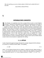
Consider
a
capacitor that
consists
of two
plane parallel electrodes
in a
vacuum having
an
applied alternating voltage represented
by the
equation
TM
Copyright n 2003 by Marcel Dekker, Inc. All Rights Reserved.
98
Chapter
3
where
v is the
instantaneous voltage,
F
m
the
maximum value
of v and
co
=

2nf
is the
angular
frequency
in
radian
per
second.
The
current through
the
capacitor,
ij
is
given
by
~)
(
3
-
2
)
2
where
m
(3.3)
z
In
this equation
C

0
is the
vacuum capacitance, some times
referred
to as
geometric
capacitance.
In
an
ideal
dielectric
the
current leads
the
voltage
by 90° and
there
is no
component
of
the
current
in
phase with
the
voltage.
If a
material
of
dielectric constant

8 is now
placed
between
the
plates
the
capacitance increases
to
CQ£
and the
current
is
given
by
(3.4)
where
(3.5)
It
is
noted that
the
usual symbol
for the
dielectric constant
is
e
r
,
but we
omit

the
subscript
for
the
sake
of
clarity, noting that
&
is
dimensionless.
The
current phasor will
not now be
in
phase with
the
voltage
but by an
angle (90°-5) where
5 is
called
the
loss
angle.
The
dielectric
constant
is a
complex quantity represented
by

E*
=
e'-je"
(3.6)
The
current
can be
resolved into
two
components;
the
component
in
phase with
the
applied
voltage
is
l
x
=
vcos"c
0
and the
component leading
the
applied voltage
by 90° is
I
y

=
vo>e'c
0
(fig.
3.1). This component
is the
charging current
of the
ideal capacitor.
TM
Copyright n 2003 by Marcel Dekker, Inc. All Rights Reserved.
Dielectric
Relaxation-I
99
The
component
in
phase with
the
applied voltage gives rise
to
dielectric
loss.
5 is the
loss
angle
and is
given
by
S

=
tan
'
—
(3.7)
s"
is
usually referred
to as the
loss
factor
and tan 8 the
dissipation factor.
To
complete
the
definitions
we
note that
d
=
Aco
8s"E
The
current density
is
given
by
J
=

— =
coss"E
Fig.
3.1
Real
(s')
and
imaginary (s") parts
of the
complex dielectric constant
(s*)
in an
alternating electric
field.
The
reference phasor
is
along
I
c
and s* =
s'
-je".
The
angle
8 is
shown
enlarged
for
clarity.

TM
Copyright n 2003 by Marcel Dekker, Inc. All Rights Reserved.
100
Chapters
The
alternating current conductivity
is
given
by
'+
&'-£„)]
(3.8)
The
total conductivity
is
given
by
3.2
POLARIZATION
BUILD
UP
When
a
direct voltage applied
to a
dielectric
for a
sufficiently
long duration
is

suddenly
removed
the
decay
of
polarization
to
zero value
is not
instantaneous
but
takes
a finite
time. This
is the
time required
for the
dipoles
to
revert
to a
random distribution,
in
equilibrium
with
the
temperature
of the
medium,
from

a field
oriented alignment.
Similarly
the
build
up of
polarization
following
the
sudden application
of a
direct voltage
takes
a finite
time interval
before
the
polarization attains
its
maximum value. This
phenomenon
is
described
by the
general term dielectric relaxation.
When
a dc
voltage
is
applied

to a
polar dielectric
let us
assume that
the
polarization
builds
up
from
zero
to a final
value (fig. 3.2) according
to an
exponential
law
J
P
ao
(l-*0
(3.9)
Where
P(t)
is the
polarization
at
time
t and T is
called
the
relaxation

time,
i
is a
function
of
temperature
and it is
independent
of the
time.
The
rate
of
build
up of
polarization
may be
obtained,
by
differentiating
equation
(3.9)
as
,
at T T
Substituting equation (3.9)
in
(3.10)
and
assuming that

the
total polarization
is due to the
dipoles,
we
get
1
TM
Copyright n 2003 by Marcel Dekker, Inc. All Rights Reserved.
Dielectric
Relaxation-I
101
dt
(3.11)
Neglecting atomic polarization
the
total polarization
P
T
(t) can be
expressed
as the sum of
the
orientational
polarization
at
that instant,
P^
(t),
and

electronic
polarization,
P
e
which
is
assumed
to
attain
its
final
value instantaneously because
the
time required
for it to
attain saturation value
is in the
optical frequency range. Further,
we
assume that
the
instantaneous polarization
of the
material
in an
alternating voltage
is
equal
to
that under

dc
voltage that
has the
same magnitude
as the
peak
of the
alternating voltage
at
that
instant.
Fig.
3.2
Polarization build
up in a
polar dielectric.
We
can
express
the
total polarization,
P
T
(t),
as
(3.12)
The
final
value attained
by the

total polarization
is
(3.13)
We
have already shown
in the
previous chapter that
the
following relationships hold
under
steady voltages:
TM
Copyright n 2003 by Marcel Dekker, Inc. All Rights Reserved.
102
Chapters
P
e
=e
0
(
S<a
-l)E
(3.14)
where
s
s
and
c^
are the
dielectric constants under direct voltage

and at
infinity
frequency
respectively.
We
further
note that
Maxwell's
relation
s^
=
n
2
(3.15)
holds true
at
optical
frequencies.
Substituting equations (3.13)
and
(3.14)
in
(3.12)
we
get
(3.16)
which
simplifies
to
j-fc

/ \
-j-^i
f
*\
-\
T\
P^
=
£
0
(s
s
-
£
X
)E
(3.17)
Representing
the
alternating electric
field as
77
77
a
^
mt
CZ
1
8
A

^
~
^max^
^J.io;
and
substituting equation
(3.18)
in
(3.11)
we get
-P(t}]
(3.19)
7
i_
-
u
\
-
j
-
ou
/
m
V/J
V
/
<^
r
The
general solution

of the first
order
differential
equation
is

(r
-r
}E
e
jcot
P(t)
= Ce
*+8
Q
l
^
^
m
(3.20)
1 +
J(DT
where
C is a
constant.
At
time
t,
sufficiently
large when compared with

i,
the first
term
on
the
right side
of
equation (3.20) becomes
so
small that
it can be
neglected
and we get
the
solution
for
P(t)
as
TM
Copyright n 2003 by Marcel Dekker, Inc. All Rights Reserved.
Dielectric
Relaxation-I
1
03
,
.
1 +
JCOT
Substituting equation
(3.21)

in
(3.12)
we get
~
E
m
e
jat
(3.22)
1 +
JCOT
Simplification
yields
i
,
\^s__~co}-[
_
77
,,j
r
»t
/"?
r
)'\\
—
1H
£Vi-c<
6
(j.Zj)
-I

.
.
-I
U
///
^
'
Equation (3.23) shows that
/Y()
is a
sinusoidal function with
the
same frequency
as the
applied voltage.
The
instantaneous value
of flux
density
D is
given
by
„ „
77
l<Ot
/">
O/l\
:
6^
0

^
E
m
e
(3.24)
But
the flux
density
is
also equal
to
Equating expressions (3.24)
and
(3.25)
we get
*
J7*
.jj^^
r.
Z7
/yJ^t
j^
J)(
+
\
C\
^f\\
substituting equation (3.23)
in
(3.26),

and
simplifying
we get
(e'-
js")
=
1
+
[e„
-1
+
g
'
~
g
°°
]
(3.27)
l +
7<yr
Equating
the
real
and
imaginary parts
we
readily obtain
£?'
—
C-

I S
CO
/O
00\
^-^00+^-
T^
i
3
-
28
)
TM
Copyright n 2003 by Marcel Dekker, Inc. All Rights Reserved.
104
Chapters
+
CO
T
It
is
easy
to
show that
-
(3-30)
£
s
Equations (3.28)
and
(3.29)

are
known
as
Debye
equations
2
and
they describe
the
behavior
of
polar dielectrics
at
various frequencies.
The
temperature
enters
the
discussion
by way of the
parameter
T as
will
be
described
in the
following section.
The
plot
of

e"
-
co
is
known
as the
relaxation curve
and it is
characterized
by a
peak
at
e'7s"
max
=
0.5.
It is
easy
to
show
COT
=
3.46
for
this ratio
and one can use
this
as a
guide
to

determine whether Debye relaxation
is a
possible mechanism.
The
spectrum
of the
Debye relaxation curve
is
very broad
as far as the
whole gamut
of
physical phenomena
are
concerned,
3
though among
the
various relaxation
formulas
Debye relaxation
is the
narrowest.
The
descriptions that
follow
in
several sections will bring
out
this aspect

clearly.
3.3
DEBYE EQUATIONS
An
alternative
and
more concise
way of
expressing Debye equations
is
8*=^+^^
(3.31)
1 +
JCOT
Equations
(3.28)-(3.30)
are
shown
in fig.
3.3.
An
examination
of
these equations shows
the
following
characteristics:
(1)
For
small values

of
COT,
the
real part
s'
«
e
s
because
of the
squared term
in the
denominator
of
equation
(3.28)
and s" is
also small
for the
same reason.
Of
course,
at
COT
= 0, we get
e"
= 0 as
expected because this
is dc
voltage.

(2) For
very
large
values
of
COT,
e' =
800
and
s"
is
small.
(3) For
intermediate values
of
frequencies
s" is a
maximum
at
some particular
value
of
COT.
The
maximum value
of s" is
obtained
at a
frequency
given

by
TM
Copyright n 2003 by Marcel Dekker, Inc. All Rights Reserved.
Dielectric
Relaxation-I
105
resulting
in
(3.32)
where
co
p
is the
frequency
at
c"
max
.
Log
m
Fig.
3.3
Schematic representation
of
Debye equations plotted
as a
function
of
logco.
The

peak
of
s"
occurs
at
COT
=
1.
The
peak
of
tan8
does
not
occur
at the
same
frequency
as the
peak
of
s".
The
values
of
s'
and s" at
this
value
of

COT
are
TM
Copyright n 2003 by Marcel Dekker, Inc. All Rights Reserved.
106
Chapters
f
'
=
^±^
(
3
-
33
)
~
The
dissipation
factor
tan 5
also increases with
frequency,
reaches
a
maximum,
and for
further
increase
in
frequency,

it
decreases.
The
frequency
at
which
the
loss angle
is a
maximum
can
also
be
found
by
differentiating
tan 6
with respect
to
co
and
equating
the
differential
to
zero. This leads
to
(3.35)
.
8(<ot)

"(
e
,+s^V)
Solving
this equation
it is
easy
to
show that
®r
=
4
p-
(3.36)
By
substituting this value
of
COT
in
equation (3.30)
we
obtain
(3.37)
The
corresponding values
of s' and
e"
are
*'
=

-^-
(3.38)
(3.39)
Fig.
3.3
also shows
the
plot
of
equation (3.30), that
is, the
variation
of tan 8 as a
function
of
frequency
for
several values
of
T.
TM
Copyright n 2003 by Marcel Dekker, Inc. All Rights Reserved.
Dielectric
Relaxation-I
107
Dividing equation
(3.28)
from
(3.27)
and

rearranging terms
we
obtain
the
simple
relationship
s"
(3.40)
s"
According
to
equation (3.40)
a
plot
of
—
against
co
results
in a
straight line
passing through
the
origin with
a
slope
of
T.
Fig.
3.3

shows that,
at the
relaxation
frequency
defined
by
equation (3.32)
e'
decreases
sharply
over
a
relatively small band width. This
fact
may be
used
to
determine whether
relaxation occurs
in a
material
at a
specified
frequency.
If we
measure
e'
as a
function
of

temperature
at
constant
frequency
it
will decrease rapidly with temperature
at
relaxation
frequency.
Normally
in the
absence
of
relaxation
s'
should increase with decreasing
temperature according
to
equation
(2.51).
Variation
of
s'
as a
function
of
frequency
is
referred
to as

dispersion
in the
literature
on
dielectrics. Variation
of s" as a
function
of
frequency
is
called absorption though
the two
terms
are
often
used interchangeably, possibly because dispersion
and
absorption
are
associated phenomena. Fig.
3.4
shows
a
series
of
measured
&'
and e" in
mixtures
of

water
and
methanol
4
.
The
question
of
determining whether
the
measured data obey Debye
equation
(3.31)
will
be
considered later
in
this chapter.
3.4
Bi-STABLE MODEL
OF A
DIPOLE
In
the
molecular model
of a
dipole
a
particle
of

charge
e may
occupy
one of two
sites,
1
or
2,
that
are
situated apart
by a
distance
b
5
.
These sites correspond
to the
lowest
potential energy
as
shown
in fig.
3.5.
In the
absence
of an
electric
field the two
sites

are
of
equal energy with
no
difference
between them
and the
particle
may
occupy
any one of
them.
Between
the two
sites, therefore, there
is a
particle.
An
applied electric
field
causes
a
difference
in the
potential energy
of the
sites.
The figure
shows
the

conditions with
no
electric
field
with
full
lines
and the
shift
in the
potential energy
due to the
electric
field
by
the
dotted line.
TM
Copyright n 2003 by Marcel Dekker, Inc. All Rights Reserved.
108
Chapter
3
"•
60
lOOX-
90X
-
eox-
60X
SOX

40X
30X
20X
40
H
10Xl
(•
ox .
Volume
friction
of
w«ur
(b)
100
100
1000
Fr*qu«ncr<UHz)
10000
1000
Prequ«ney(tlHz)
10000
•: 00X
w«Ur
b: SOX
w«ter
e:
10X
water
20
40

60
60
100
Fig.
3.4
Dielectric properties
of
water
and
methanol mixtures
at
25°C.
(a)
Real part,
s' (b)
Imaginary
part,
s" (c)
Complex plane plot
of s*
showing Debye relaxation (Bao
et.
al.,
1996).
(with permission
of
American Physical Society.)
The
difference
in the

potential
energy
due to the
electric
field E is
i
~~02
=ebEcos0
TM
Copyright n 2003 by Marcel Dekker, Inc. All Rights Reserved.
Dielectric
Relaxation-I
109
where
0 is the
angle between
the
direction
of the
electric
field and the
line joining
1 and
2.
This model
is
equivalent
to a
dipole changing position
by

180°
when
the
charge moves
from
site
1 to 2 or
from
site
2 to
1.
The
moment
of
such
a
dipole
is
f*
=
-eb
which
may be
thought
of as
having been hinged
at the
midpoint between sites
1 and 2.
This model

is
referred
to as the
bistable model
of the
dipole.
We
also assume that
0
=
0
for
all
dipoles
and
that
the
potential energy
of
sites
1 and 2 are
equal
in the
absence
of an
external electric
field.
Electric
Field
a*

1
d
I
position
Fig.
3.5 The
potential well model
for a
dipole with
two
stable
positions.
In the
absence
of an
electric
field
(foil
lines)
the
dipole spends equal time
in
each well;
this
indicates that there
is no
polarization.
In the
presence
of an

electric
field
(broken lines)
the
wells
are
tilted with
the
'downside'
of the field
having
a
slightly lower energy than
the
'up'
side; this
represents
polarization.
I
TM
Copyright n 2003 by Marcel Dekker, Inc. All Rights Reserved.
HO
Chapters
We
assume that
the
material contains
N
number
of

bistable dipoles
per
unit volume
and
the
field
due to
interaction
is
negligible.
A
macroscopic consideration shows that
the
charged particles would
not
have
the
energy
to
jump
from one
site
to the
other. However,
on
a
microscopic scale
the
dipoles
are in a

heat reservoir exchanging energy with each
other
and
dipoles.
A
charge
in
well
1
occasionally acquires enough energy
to
climb
the
hill
and
moves
to
well
2.
Upon arrival
it
returns energy
to the
reservoir
and
remain there
for
some time.
It
will then acquire energy

to
jump
to
well
1
again.
The
number
of
jumps
per
second
from one
well
to the
other
is
given
in
terms
of the
potential energy
difference
between
the two
wells
as
kT
where
T is the

absolute temperature,
k the
Boltzmann
constant
and A is a
factor denoting
the
number
of
attempts.
Its
value
is
typically
of the
order
of
10~
13
s"
1
at
room temperature
though values
differing
by
three
or
four
orders

of
magnitude
are not
uncommon.
It may
or
may not
depend
on the
temperature.
If it
does,
it is
expressed
as B/T as
found
in
some
polymers.
If the
destination well
has a
lower energy than
the
starting well then
the
minus
sign
in the
exponent

is
valid.
The
relaxation time
is the
reciprocal
of
Wi
2
leading
to
forw
The
variation
of
T
with
T in
liquids
and in
polymers near
the
glass transition temperature
is
assumed
to be
according
to
this equation. Other
functions

of T
have also been
proposed which
we
shall consider
in
chapter
5. The
decrease
of
relaxation time with
increasing temperature
is
attributed
to the
fact
that
the
frequency
of
jump increases with
increasing temperature.
3.5
COMPLEX PLANE DIAGRAM
Cole
and
Cole showed that,
in a
material exhibiting Debye relaxation
a

plot
of
e"
against
c',
each point corresponding
to a
particular
frequency
yields
a
semi-circle. This
can
easily
be
demonstrated
by
rearranging equations (3.28)
and
(3.29)
to
give
/~»\2
,
f
„!
„
\1
_
(

£
S
~
£
ao)
TM
Copyright n 2003 by Marcel Dekker, Inc. All Rights Reserved.
Dielectric
Relaxation-I
111
The
right side
of
equation
(3.41)
may be
simplified
using equation (3.28) resulting
in
(G"}
2
+
(8'
-
O
2
=
(*,
-
*.)(*'

-
O
(3.42)
Further simplification yields
*'
2
-*'(*,+O
+
*A,+*'
r2
=
0
(3-43)
Substituting
the
algebraic identity
£,£
a
,=-[(£
3
+£j
2
-(£
s
+£j
2
]
equation
(3.43)
may be

rewritten
as
(£
'
_
£t±f«
)2
+
(
£
»y
=
(£LZ^.)2
(3
44)
G — G G
~\~
G
This
is the
equation
of a
circle with radius
—
—
having
its
center
at
(—

—
,0 ).
It can
easily
be
shown that
(SOD,
0) and
(e
s
,
0) are
points
on the
circle.
To put it
another
way,
the
circle intersects
the
horizontal axis
(s')
at
Soo
and
s
s
as
shown

in fig.
3.6.
Such
plots
of s"
versus
e'
are
known
as
complex plane plots
of s*.
At
(Dpi
= 1 the
imaginary component
s"
has a
maximum value
of
The
corresponding value
of
s'
is
Of
course these results
are
expected because
the

starting point
for
equation
(3.44)
is the
original
Debye equations.
TM
Copyright n 2003 by Marcel Dekker, Inc. All Rights Reserved.
112
Chapter
3
001?=
1
increases
(
e,+
e
J/2
Fig.
3.6
Cole-Cole diagram displaying
a
semi-circle
for
Debye equations
for s*.
In
a
given material

the
measured values
of
s"
are
plotted
as a
function
of
s'
at
various
frequencies,
usually
from
w
= 0 to
eo
=
10
10
rad/s.
If the
points
fall
on a
semi-circle
we
can
conclude

that
the
material exhibits Debye relaxation.
A
Cole-Cole diagram
can
then
be
used
to
obtain
the
complex dielectric constant
at
intermediate frequencies obviating
the
necessity
for
making measurements.
In
practice very
few
materials completely agree
with Debye equations,
the
discrepancy being attributed
to
what
is
generally referred

to as
distribution
of
relaxation times.
The
simple theory
of
Debye assumes that
the
molecules
are
spherical
in
shape
and
therefore
the
axis
of
rotation
of the
molecule
in an
external
field
has no
influence
in
deciding
the

value
of e .
This
is
more
an
exception than
a
rule because
not
only
the
molecules
can
have
different
shapes, they have, particularly
in
long chain polymers,
a
linear
configuration. Further,
in the
solid phase
the
dipoles
are
more likely
to be
interactive

and not
independent
in
their response
to the
alternating
field
7
.
The
relaxation
times
in
such materials have
different
values depending upon
the
axis
of
rotation and,
as
a
result,
the
dispersion commonly occurs over
a
wider
frequency
range.
TM

Copyright n 2003 by Marcel Dekker, Inc. All Rights Reserved.
Dielectric
Relaxation-I
113
3.6
COLE-COLE RELAXATION
Polar dielectrics that have more than
one
relaxation time
do not
satisfy
Debye equations.
They show
a
maximum value
of
e"
that will
be
lower than that predicted
by
equation
(3.34).
The
curve
of tan 5 vs log
COT
also shows
a
broad maximum,

the
maximum value
being smaller than that given
by
equation (3.37). Under these conditions
the
plot
e"
vs.
s'
will
be
distorted
and
Cole-Cole showed that
the
plot will still
be a
semi-circle with
its
center displaced below
the
s'
axis. They suggested
an
empirical equation
for the
complex dielectric constant
as
~

,
;0<a<l;
(3.45)
\l
—
c/
~ ~
\.
s
]
a
—
0 for
Debye
relaxation
where
i
c
.
c
is the
mean relaxation time
and
a
is a
constant
for a
given material, having
a
value

0
<
a
<
1.
A
plot
of
equation
(3.45)
is
shown
in figs.
(3.7)
and
(3.8)
for
various
values
of a.
Debye equations
are
also plotted
for the
purpose
of
comparison. Near
relaxation frequencies Cole-Cole relaxation shows that
s'
decreases more slowly with

co
than
the
Debye relaxation. With increasing
a the
loss
factor
e"
is
broader than
the
Debye
relaxation
and the
peak value,
s
max
is
smaller.
A
dielectric that
has a
single relaxation time,
a = 0 in
this
case,
equation (3.45) becomes
identical with equation (3.29).
The
larger

the
value
of a, the
larger
the
distribution
of
relaxation times.
To
determine
the
geometrical interpretation
of
equation
(3.45)
we
substitute
l-a
= n and
rewrite
it as
(3-46)
/
vi,
•
•
^
(o)T
c
_

c
)
(cos—
+
7
sin—
)
Equating real
and
imaginary parts
we get
TM
Copyright n 2003 by Marcel Dekker, Inc. All Rights Reserved.
114
Chapter
3
(3.47)
2(a)T
c
_
c
)"
cos(
wr
/
2)
v2«
(3.48)
Fig.
3.7

Real part
of s* in a
polar dielectric according
to
Cole-Cole
relaxation,
a =0
gives
Debye
relaxation.
Using
the
identity
j
a
=
o
equations
(3.47)
and
(3
.48)
may be
expressed alternatively
as
s
-,
sinhn-s
cosh
«5

+ si
/ 2)
(3.46a)
TM
Copyright n 2003 by Marcel Dekker, Inc. All Rights Reserved.
Dielectric
Relaxation-I
115
s
s
-
s"
_ 1
(
cos(cr;r/2)
2\^
cosh
ns +
sin(a;r
/ 2)
(3.47a)
where
5
=
Lncor
X
11=0.75
""-
n=l
(Dtbve)

Jt
l
HF
10
Fig.
3.8
Imaginary part
of s* in a
polar dielectric according
to
Cole-Cole
relaxation,
a =0
gives
Debye
relaxation.
Eliminating
OOT
C
.
C
from
equations (3.47)
and
(3.48)
Cole-Cole showed that
(3.49)
Equation (3.49) represents
the
equation

of a
circle with
the
center
at
TM
Copyright n 2003 by Marcel Dekker, Inc. All Rights Reserved.
116
Chapter
3
and
having
a
radius
of
We
note that
the y
coordinate
of the
center
is
negative, that
is, the
center lies below
the
s'
axis
(fig. 3.9).
Figs.

3.7 and 3.8
show
the
variation
of
s'
and
e"
as a
function
of
cox
for
several values
of
a
respectively. These
are the
plots
of
equations (3.47)
and
(3.48).
At
COT
= 1 the
following
relations hold:
„
£•

-
£•
nn
8
=
—
—
tan
—
/2,
cot(n7T/2)x(-
e
s
+eJ/2
Fig.
3.9
Geometrical relationships
in
Cole-Cole equation (3.45).
TM
Copyright n 2003 by Marcel Dekker, Inc. All Rights Reserved.
Dielectric
Relaxation-I
117
As
stated above,
the
case
of
n

= 0
corresponds
to an
infinitely
large number
of
distributed relaxation times
and the
behavior
of the
material
is
identical
to
that under
dc
fields
except that
the
dielectric constant
is
reduced
to
(s
s
-
Soo)/2.
The
complex part
of the

dielectric constant
is
also equal
to
zero
at
this value
of
n,
consistent with
dc
fields.
As the
value
of n
increases
s'
changes with increasing
COT,
the
curves crossing over
at
COT
= 1. At
n=l the
change
in
s'
with increasing
COT

is
identical
to the
Debye relaxaton,
the
material
then
possessing
a
single relaxation time.
The
variation
of s"
with
COT
is
also dependent
on the
value
of n. As the
value
of n
increases
the
curves become narrower
and the
peak value increases. This behavior
is
consistent with that shown
in

fig.
3.8.
Let
the
lines joining
any
point
on the
Cole-Cole diagram
to the
points corresponding
to
Soo
and
s
s
be
denoted
by u and v
respectively (Fig. 3.9). Then,
at any
frequency
the
following
relations hold:
oo
'
/
M
u

=
s
-s-
v
=
r^;
—
=
(COT}
-c
/
\
I—
n
^
'
(COT)
u
By
plotting
log
co
against (log
v-log
u) the
value
of n may be
determined. With
increasing value
of n, the

number
of
degrees
of
freedom
for
rotation
of the
molecules
decreases. Further decreasing
the
temperature
of the
material leads
to an
increase
in the
value
of the
parameter
n.
The
Cole-Cole diagrams
for
poly(vinyl
chloride)
at
various temperatures
are
shown

in
fig.
3.10
9
.
The
Cole-Cole
arc is
symmetrical about
a
line
through
the
center parallel
to
the
s"
axis.
3.7
DIELECTRIC PROPERTIES
OF
WATER
Debye relaxation
is
generally limited
to
weak solutions
of
polar liquids
in

non-polar
solvents. Water
in
liquid state comes closest
to
exhibiting Debye relaxation
and its
dielectric properties
are
interesting because
it has a
simple molecular structure.
One is
fascinated
by the
fact
that
it
occurs naturally
and
without
it
life
is not
sustained. Hasted
(1973)
quotes over thirty determinations
of
static dielectric constant
of

water, already
referred
to in
chapter
2.
TM
Copyright n 2003 by Marcel Dekker, Inc. All Rights Reserved.
118
Chapter
3
n
s'
Fig.
3.10
Cole-Cole diagram
from
measurements
on
poly (vinyl chloride)
at
various temperatures
(Ishida, 1960). (With permission
of Dr.
Dietrich
Steinkopff
Verlag, Darmstadt, Germany).
The
dielectric constant
is not
appreciably dependent

on the
frequency
up to 100
MHz.
The
measurements
are
carried
out in the
microwave
frequency
range
to
determine
the
relaxation frequency,
and a
particular disadvantage
of the
microwave
frequency
is
that
individual
observers
are
forced,
due to
cost,
to

limit their studies
to a
narrow
frequency
range. Table
3.1
summarizes
the
data
due to
Bottreau
et.
al.
(1975).
TM
Copyright n 2003 by Marcel Dekker, Inc. All Rights Reserved.
Dielectric
Relaxation-1
119
Table
3.1
Selective
Dielectric
Properties
of
Water
at 293 K
(Bottreau,
et.
al.,

1975).
800
=
n
2
=
1.78,
e
s
=
80.4
(With permission
of
Journal
of
Chemical
Physics,
USA)
/(GHz)
2530.00
890.00
300.00
35.25
34.88
24.19
23.81
23.77
23.68
23.62
15.413

9.455
9.390
9.375
9.368
9.346
9.346
9.141
4.630
3.624
3.254
1.744
1.200
0.577
13760
6880
3440
Measured
complex
permittivity
s'
3.65
4.30
5.48
20.30
19.20
29.64
30.50
31.00
31.00
30.88

46.00
63.00
61.50
62.00
62.80
61.41
62.26
63.00
74.00
77.60
77.80
79.20
80.4
80.3
Extrapolated
1.98
2.37
3.25
S"
1.35
2.28
4.40
29.30
30.30
35.18
35.00
35.70
35.00
35.75
36.60

31.90
31.60
32.00
31.50
31.83
32.56
31.50
18.80
16.30
13.90
7.90
7.00
2.75
values
from
0.75
1.15
1.45
Measured
reduced
permittivity
Em'
0.0238
0.0321
0.0471
0.2356
0.2216
0.3544
0.3653
0.3717

0.3717
0.3701
0.5625
0.7787
0.7596
0.7660
0.7761
0.7585
0.7693
0.7787
0.9186
0.9644
0.9669
0.9847
1.000
0.9987
F
"
l-TCl
0.0172
0.0290
0.0560
0.3727
0.3854
0.4475
0.4452
0.4541
0.4452
0.4547
0.4655

0.4057
0.4019
0.4070
0.4007
0.4049
0.4141
0.4007
0.2391
0.2073
0.1768
0.1005
0.0890
0.0350
Calculated reduced
permittivity
E
c
'
0.0230
0.0335
0.0384
0.2230
0.2262
0.3600
0.3667
0.3674
0.3690
0.3701
0.5645
0.7618

0.7641
0.7646
0.7649
0.7656
0.7656
0.7728
0.9215
0.9486
0.9576
0.9868
0.9936
0.9985
EC"
0.0234
0.0272
0.0582
0.3764
0.3787
0.4478
0.4500
0.4502
0.4507
0.4510
0.4683
0.4003
0.3989
0.3986
0.3984
0.3980
0.3980

0.3934
0.2472
0.2016
0.1835
0.1030
0.0717
0.0348
a
single relaxation
of
Debye type
0.0026
0.0077
0.0188
0.0095
0.0146
0.0184
0.0021
0.0071
0.0179
0.0096
0.0167
0.0227
The
following
definitions
apply
for the
quantities
in

shown Table
3.1.
'=^^;
E*
=
£
~
8
TM
Copyright n 2003 by Marcel Dekker, Inc. All Rights Reserved.
120
Chapter
3
10
and
is
reproduced
from
ref.
.
Fig.
3.11
shows
the
complex plane plots
of e' -
js"
for
water (Hasted,
1973)

and
compared with analysis according
to
Debye equations
and
Cole-Cole equations.
The
relaxation time obtained
as a
function
of
temperature
from
Cole-Cole analysis
is
shown
in
Table
3.2
along with
£
w
used
in the
analysis.
Table
3.2
Relaxation time
in
water

(Hasted,
1973)
T°C
0
10
20
30
40
50
60
75
GOO
4.46
+
0.17
4.10±0.15
4.23+0.16
4.20
±0.16
4.16±0.15
4.13±0.15
4.21
±0.16
4.49
+
0.17
T(10-
n
)s
1.79

1.26
0.93
0.72
0.58
0.48
0.39
0.32
a
0.014
0.014
0.013
0.012
0.009
0.013
0.011
-
(permission
of
Chapman
and
Hall)
*
msn
I
-
cat
|
MENTsi
Fig.
3.11

Complex plane
plot
of s* in
water
at
25°C
in the
microwave
frequency
range.
Points
in
closed circles
are
experimental
data,
x,
calculations
from
Cole-Cole plot,
+,
calculations
from
Debye equation with optimized parameters [Hasted
1973].
(with permission
of
Chapman
&
Hall, London).

TM
Copyright n 2003 by Marcel Dekker, Inc. All Rights Reserved.
Dielectric
Relaxation-I
121
Earlier literature
on c* in
water
did not
extend
to as
high
frequencies
as
shown
in
Table
3.1
and it was
thought that
£<»
is
much greater than
the
square
of
refractive
index,
n
— 1.8

(Hasted, 1973),
and
this
was
attributed
to,
possibly absorption
and a
second dipolar
dispersion
of
e"
at
higher
frequencies. However more recent measurements
up to
2530
GHz and
extrapolation
to
13760
GHz
shows that
the
equation
800
=
n
2
is

valid,
as
demonstrated
in
Table
3.1.
The
relaxation time increases with decreasing temperature
in
qualitative
agreement with
the
Debye concept.
The
Cole-Cole parameter
a is
relatively
small
and
independent
of
temperature. Recall that
as
a—»
0 the
Cole-Cole distribution
converges
to
Debye relaxation.
At

this point
it is
appropriate
to
introduce
the
concept
of
spectral decomposition
of the
complex plane plot
of s*. If we
suppose that there
exist
several relaxation processes,
each with
a
characteristic relaxation time
and
dominant over
a
specific
frequency
range,
then
the
Debye equation
(3.31)
may be
expressed

as
+
CO
Tj
•an,
(3.51)
where
Acs
and
i\
are the
individual amplitude
of
dispersion
(si
ow
frequency
-
Shigh
frequency)
and
the
relaxation time, respectively.
The
assumption here
is
that each relaxation process
follows
the
Debye equation independent

of
other
processes.
This kind
of
representation
has
been used
to find the
relaxation times
in
D
2
O
ice
11
.
Polycrystalline
ice
from
water
has
been shown
to
have
a
single relaxation time
of
Debye
type

at 270
K
12
and the
observed distribution
of
relaxation times
at
lower temperatures
165-196
K is
attributed
to
physical
and
chemical
impurities
13
.
However
the
D
2
O
ice
shows
a
more interesting behavior. Focusing
our
attention

to the
point under discussion,
namely
several relaxation times,
fig.
3.12
shows
the
measured values
of
s'
and s" in the
complex
plane
as
well
as the
three relaxation processes.
The
As
and
i
are
88.1,
57.5
and
1.4
(see inset) and,
20 ms, 60 ms and 100 us
respectively.

A
method
of
spectral analysis which
is
similar
in
principle
to
what
was
described above,
but
different
in
procedure,
has
been adopted
by
Bottreau
et.
al.
(1975)
who use a
function
of
the
type
TM
Copyright n 2003 by Marcel Dekker, Inc. All Rights Reserved.