dielectrics in electric fields (11)

10
THERMALLY
STIMULATED
PROCESSES
T
hermally
stimulated processes (TSP)
are
comprised
of
catalyzing
the
processes
of
charge generation
and its
storage
in the
condensed phase
at a
relatively higher
temperature
and
freezing
the
created charges, mainly
in the
bulk
of the
dielectric
material,

at a
lower
temperature.
The
agency
for
creation
of
charges
may be
derived
by
using
a
number
of
different
techniques; Luminescence, x-rays, high electric
fields
corona
discharge, etc.
The
external agency
is
removed
after
the
charges
are
frozen

in and the
material
is
heated
in a
controlled manner during which
drift
and
redistribution
of
charges
occur within
the
volume. During heating
one or
more
of the
parameters
are
measured
to
understand
the
processes
of
charge generation.
The
measured parameter,
in
most cases

the
current,
is a
function
of
time
or
temperature
and the
resulting curve
is
variously
called
as the
glow curve,
thermogram
or the
heating curve.
In the
study
of
thermoluminescence
the
charge carriers
are
generated
in the
insulator
or
semiconductor

at
room temperature using
the
photoelectric
effect.
The
experimental aspects
of TSP are
relatively simple though
the
number
of
parameters
available
for
controlling
is
quite large.
The
temperature
at
which
the
generation
processes
are
catalyzed, usually called
the
poling temperature,
the

poling
field,
the
time
duration
of
poling,
the
freezing temperature (also called
the
annealing temperature),
and
the
rate
of
heating
are
examples
of
variables
that
can be
controlled.
Failure
to
take
into
account
the
influences

of
these parameters
in the
measured
thermograms
has led to
conflicting
interpretations
and in
extreme
cases,
even
the
validity
of the
concept
of TSP
itself
has
been questioned.
In
this chapter
we
provide
an
introduction
to the
techniques that have been adopted
in
obtaining

the
thermograms
and the
methods applied
for
their analysis. Results obtained
in
specific
materials have been used
to
exemplify
the
approaches adopted
and
indicate
TM
Copyright n 2003 by Marcel Dekker, Inc. All Rights Reserved.
the
limitations
of the TSP
techniques
1
'
2
'
3
.
To
limit
the

scope
of the
chapter
we
limit
ourselves
to the
presentation
of the
Thermally Stimulated Depolarization (TSD) Current.
In
what
follows
we
adopt
the
following terminology:
The
electric
field,
which
is
applied
to the
material
at the
higher temperature,
is
called
the

poling
field.
The
temperature
at
which
the
generation
of
charges
is
accelerated
is
called
the
poling temperature and,
in
polymers, mostly
the
approximate
glass
transition
temperature
is
chosen
as the
poling temperature.
The
temperature
at

which
the
electric
field
is
removed
after
poling
is
complete
is
called
the
initial temperature because heating
is
initiated
at
this temperature.
The
temperature
at
which
the
material
is
kept short circuited
to
remove stray charges,
after
attaining

the
initial temperature
and the
poling
field
is
removed,
is
called
the
annealing temperature.
The
annealing temperature
may or may not be the
initial
temperature.
The
current released during heating
is a
function
of the
number
of
traps
(n
t
).
If the
current
is

linearly dependent
on
n
t
then
first
order kinetics
is
said
to
apply.
If the
current
is
dependent
on
n
t
(Van
Turnhout,
1975)
then second order kinetics
is
said
to
apply.
10.1
TRAPS
IN
INSULATORS

The
concept
of
traps
has
already been introduced
in
chapter
7 in
connection with
the
discussion
of
conduction currents.
To
facilitate understanding
we
shall begin with
the
description
of
thermoluminiscence
(Chen
and
Kirsch,
1981).
Let us
consider
a
material

in
which
the
electrons
are at
ground state
G and
some
of
them acquire energy,
for
which
we
need
not
elaborate
the
reasons,
and
occupy
the
level
E
(Fig.
10.1).
The
electrons
in
the
excited state,

after
recombinations, emit photons within
a
short time interval
of
10"
8
s
and
return
to the
ground
state. This phenomenon
is
known
as florescence and
emission
of
light ceases
after
the
exciting radiation
has
been switched off.
The
electrons
may
also lose some energy
and
fall

to an
energy level
M
where
recombination
does
not
occur
and the
life
of
this
excited state
is
longer.
The
energy level
corresponding
to M may be due to
metastables
or
traps.
Energy equivalent
to s
needs
to
be
imparted
to
shift

the
electrons
from
M to E,
following which
the
electrons undergo
recombination.
In
luminescence this phenomenon
is
recognized
as
delayed emission
of
light
after
the
exciting radiation
has
been turned off.
In the
study
of
TSDC
and TSP the
energy
level corresponding
to M is, in a
rather unsophisticated sense, equivalent

to
traps
TM
Copyright n 2003 by Marcel Dekker, Inc. All Rights Reserved.
of
single energy.
The
electrons stay
in the
trap
for a
considerable time which results
in
delayed response.
The
probability
of
acquiring energy,
s
a
,
thermally
to
jump
from
a
trap
may be
expressed
as

(10.1)
where
n is the
number
of
electrons released
at
temperature
T,
n
0
the
initial number
of
traps
from
which electrons
are
released
(n/n
0
<
1), s is a
constant,
k the
Boltzmann
constant
and T the
absolute temperature.
Eq.

(10.1)
shows that
the
probability increases
with
increasing temperature.
The
constant
s is a
function
of
frequency
of
attempt
to
escape
from
the
trap, having
the
dimension
of
s"
1
.
A
trap
is
visualized
as a

potential well
from
which
the
electron attempts
to
escape.
It
acquires energy thermally
and
collides
with
the
walls
of the
potential
well,
s is
therefore
a
product
of the
number
of
attempts
multiplied
by the
reflection
coefficient.
In

crystals
it is
about
an
order
of
magnitude less
than
the
vibrational
frequency
of the
atoms,
~
10
12
s"
1
.
The
so
called
first
order kinetics
is
based
on the
simplistic assumption that
the
rate

of
release
of
electrons
from
the
traps
is
proportional
to the
number
of
trapped electrons.
This results
in the
equation
^-=-an(t)
(10.2)
dt
where
the
constant,
a
represents
the
decrease
in the
number
of
trapped electrons

and has
the
dimension
of
s'
1
.
The
solution
of eq.
(10.2)
is
n(t)=n
0
exp(-at)
(10.3)
where
n
0
is the
number
of
electrons
at t = 0.
In
terms
of
current, which
is the
quantity usually measured, equation (10.3)

may be
rewritten
as
-
(10.4)
/
j
I
A
/
rri
\
s
dt
T
TM
Copyright n 2003 by Marcel Dekker, Inc. All Rights Reserved.
where
i
is
called
the
relaxation time, which
is the
reciprocal
of the
jump frequency
and C
a
proportionality

constant.
Let us
assume
a
constant heating rate
p\
We
then have
T
=
T
0
+fit
where
T
0
and t are the
initial
temperature
and
time
respectively.
(10.5)
E
2
M
G
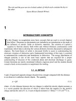
Fig.
10.1
Energy states

of
electrons
in a
solid.
G is the
ground state,
E the
excited level
and M
the
metastable level. Excitation
shifts
the
electrons
to E via
process
1.
Instantaneous return
to
ground
state-process
2
results
in
fluorescence. Partial loss
of
energy transfers
the
electron
to

M
via
process
3.
Acquiring energy
e
the
electron reverts
to
level
E
(process
4).
Recombination with
a
hole results
in the
emission
of a
photon (Process
5) and
phosphorescence. Adopted
from
Chen
and
Kirsch
(1981),
(with permission
of
Pergamon

Press)
The
solution
of
equation
(10.4)
is
given
as
kT
(10.6)
This
equation
is
known
as the
first
order
kinetics.
The
second
order kinetics
is
based
on
the
concept that
the
rate
of

decay
of the
trapped electrons
is
dependent
on the
population
TM
Copyright n 2003 by Marcel Dekker, Inc. All Rights Reserved.
of
the
excited electrons
and
vacant impurity levels
or
positive holes
in a
filled
band. This
leads
to the
equation
~)
/
"
dn n
\
£,
I-
=

exp
—
dt T ( kT
(10.7)
3
„-!
where
T' is a
constant having
the
dimension
of m s" . The
solution
of
this equation
is
n
f
2-
kT
kT'
-2
(10.8)
without losing generality, equations (10.6)
and
(10.8)
are
expressed
as
dn

( n
|
n
(
s
=
=
—
^exp
—-
dt
(nj
T
\
kT,
(10.9)
where
the
exponent
b is the
order
of
kinetics.
Returning
to
Fig.
(10.1)
the
metastable level
M may be

equated
to
traps
in
which
the
electrons stay
a
long time relative
to
that
at E. The
trapping level, having
a
single energy
level
c, and a
single retrapping center (Fig.
10.1)
shows
a
single peak
in the
measured
current
as a
function
of the
temperature.
The

trap energy level
is
determined, according
to
equation
(10.1)
for
n
T
,
by the
slope
of the
plot
of
In
(I)
versus
I/T.
A
polymer having
a
single trap level
and
recombination center
is a
simplified
picture,
used
to

render
the
mathematical analysis easier.
In
reality,
the
situation that
one
obtains
is
shown
in
Fig.
10.2
where
n
c
denotes
the
number
of
electrons
in the
conduction band.
The
trap levels,
TI,
T
2
,

. . . are
situated closer
to the
conduction band
and the
holes,
HI,
H
2
,
. . . are
retrapping centers. Introduction
of
even this moderate level
of
sophistication
requires that
the
following
situations should
be
considered (Chen
and
Kirsch,
1981).
1.
The
trap levels have discreet energy
differences
in

which case each level could
be
identified
with
a
distinct peak
in the
thermogram.
On the
other hand
the
trap levels
may
form
a
local continuum
in
which case
the
current
at any
temperature
is a
contribution
of a
number
of
trap levels.
The
peak

in the
thermogram
is
likely
to be
broad.
2.
The
traps
are
relatively closer
to the
conduction band
so
that thermally activated
electron
transfer
can
occur.
The
holes
are
situated
not
quite
so
close
to the
valence
TM

Copyright n 2003 by Marcel Dekker, Inc. All Rights Reserved.
band
so
that
the
holes
do not
contribute
to the
current
in the
range
of
temperatures
used
in the
experiments.
The
reverse situation, though
not so
common,
may
obtain;
the
holes
are
closer
to the
valence band
and

traps
are
deep.
The
electron
traps
now
become recombination centers completing
the
"mirror image".
3.
The
essential
feature
of a
thermogram
is the
current peak, which
is
identified
with
the
phenomenon
of
trapping
and
subsequent release
due to
thermal activation.
The

sign
of the
carrier, whether
it is a
hole
or
electron,
is
relatively
of
minor
significance.
In
this context
the
trapping levels
may be
thermally active
in
certain
ranges
of
temperature while,
in
other ranges, they
may be
recombination
centers.
4. An
electron which

is
liberated
from
a
trap
may
drift
under
the field
before
being
trapped
in
another center that
has the
same energy level.
The
energy level
of the
new
trap
may be
shallower, that
is
closer
to the
conduction band. This mode
of
drift
has led to the

term
"hopping".
The
development
of
adequate theories
to
account
for
these complicated situations
is, by
no
means, straight
forward.
However, certain basic concepts
are
common
and
they
may
be
summarized
as
below:
1)
The
intensity
of
current
is a

function
of the
number
of
traps according
to
equation 10.4.
The
implied condition that
the
number density
of
traps
and
holes
is
equal
is not
necessarily true.
To
render
the
approach general
let us
denote
the
number
of
traps
by

n
t
and the
number
of
holes
by
nn.
The
number
of
holes will
be
less
if a
free
electron
recombines
with
a
hole. Equation (10.7)
now
becomes
(10.10)
at
where
n
c
is the
number density

of
free
carriers
in the
conduction band
and
f
rc
is the
recombination
probability with
the
dimension
of m
3
s"
1
.
The
recombination probability
is
the
product
of the
thermal velocity
of
free
electrons
in the
conduction band,

v, and the
recombination
cross section
of the
hole,
a
rc
.
2)
The
electrons
from
the
traps move
to the
conduction band
due to
thermal activation.
The
change
in the
density
of
trapped carriers,
n
t
,
is
dependent
on the

number density
of
trapped charges
and the
Boltzmann factor. Retrapping also reduces
the
number that
moves into
the
conduction level.
The
retrapping probability
is
dependent
on the
number
density
of
unoccupied traps. Unoccupied trap density
is
given
by
(N-n
t
)
where
N is the
concentration
of
traps under consideration.

The
rate
of
decrease
of
electrons
from
the
traps
is
given
by
TM
Copyright n 2003 by Marcel Dekker, Inc. All Rights Reserved.
c{
(10.11)
at
v
kT
)
where
f
rt
is the
retrapping probability
(m
3
s"
1
).

Similar
to the
recombination probability,
we
can
express
f
n
as the
product
of the
retrapping cross section,
a
rt
,
and the
thermal
velocity
of the
electrons
in the
conduction band.
3) The net
charge
in the
medium
is
zero.
Accordingly
n

c+
n
t
-n
h
=Q
(10.12)
This equation transforms into
dn
lL=
dn
L+
dn^
(1013)
dt
dt
dt
Substituting equation
(10.1
1)
in
(10.13)
gives
=
sn
expf
-
-i-1
-
n

c
(n
h
f
rc
+
(N-n,
)/„
(10.14)
at V kT
Equations (10.10), (10.13)
and
(10.14)
are
considered
to be
generally applicable
to
thermally stimulated
processes,
with modifications introduced
to
take into account
the
specific
conditions.
For
example
the
charge neutrality condition

in a
solid with number
of
trap levels,
T
1?
T
2
,

etc.,
and a
number
of
hole levels
HI,
H
2

etc., (Fig. 10.2)
is
given
by
*=°
(10-15)
Numerical
solutions
for the
kinetic equations governing thermally stimulated
are

given
by
Kelly,
et
al.
(1972)
and
Haridoss
(1978)
4
'
5
.
Invariably some approximations need
to
be
made
to
find
the
solutions
and
Kelly,
et al.
(1971) have determined
the
conditions
under
which
the

approximations
are
valid.
The
model employed
by
them
is
shown
in
Fig.
10.3.
Let N
number
of
traps
be
situated
at
depth
E
below
the
conduction band, which
has
a
density
of
states,
N

c
.
On
thermal stimulation
the
electrons
are
released
from
the
traps
to
the
conduction band with
a
probability lying between zero
and
one,
according
to the
Boltzmann factor
e'
EM
'
.
The
electrons move
in the
conduction band under
the

influence
of an
electric
field,
during which event they
can
either drop into recombination centers with
a
capture
TM
Copyright n 2003 by Marcel Dekker, Inc. All Rights Reserved.
coefficient
y or be
retrapped with
a
coefficient
of [3. The
relative magnitude
of the two
coefficients
depend
on the
nature
of the
material; retrapping
is
dominant
in
dielectrics
whereas

recombination
with
light
output
dominates
in
thermoluminiscent
materials.
Conduction level
Forbidden
energy
gap
Valence
level
Fig.
10.2 Electron trap levels
(T) and
hole levels
(H) in the
forbidden
gap of an
insulator.
N
c
is
the
number density
of
electrons
in the

conduction band.
The
number density
of
electrons
in
TI
is
denoted
by the
symbol
n
t
i
and
hole density
in
HI
is
nhi.
Charge conservation
is
given
by
equation (10.15). Adopted
from
(Chen
and
Kirsch, 1981, with permission
of

Pergamon Press,
Oxford).
CONDUCTION
BAND
n
c
,N
c
P
N
M
Fig.
10.3 Energy level diagram
for the
numerical analysis
of
Kelly
et.
al.
(1972), (with permission
of
Am.
Inst.
of
Phy.)
TM
Copyright n 2003 by Marcel Dekker, Inc. All Rights Reserved.
In
the
absence

of
deep traps,
the
occupation numbers
in the
traps
and the
conduction
band
are
n
and
n
c
respectively. Note that
the
energy diagram shown
in fig.
10.3
is
relatively
more detailed than
those
shown
in
Figs.
10.1
and
10.2.
10.2 CURRENT

DUE TO
THERMALLY STIMULATED DEPOLARIZATION
(TSDC)
We
shall
focus
our
attention
on the
current released
to the
external circuit during
thermally stimulated depolarization processes.
To
provide continuity
we
briefly
summarize
the
polarization mechanisms that
are
likely
to
occur
in
solids:
1)
Electronic polarization
in the
time range

of
10"
15
<
t
<
10"
17
s
2)
Atomic
polarization,
10"
12
<
t
<
10"
14
s
3)
Orientational polarization,
10"
3
<
t
<
10"
12
s

4)
Interfacial
polarization,
t >
0.
1
s
5)
Drift
of
electrons
or
holes
in the
inter-electrode region
and
their trapping
6)
Injections
of
charges into
the
solid
by the
electrodes
and
their trapping
in the
vicinity
of the

electrodes. This mechanism
is
referred
to as
electrode polarization.
Considering
the
orientational polarization
first,
generally
two
experimental techniques
are
employed, namely, single temperature poling (Fig. 10.4)
and
windowing
6
(Fig. 10.5).
The
windowing technique, also called
fractional
polarization,
is
meant
to
improve
the
method
of
separating

the
polarizations that occur
in a
narrow window
of
temperature.
The
width
of the
window chosen
is
usually 10°C. Even
in the
absence
of
windowing
technique, several techniques have been adopted
to
separate
the
peaks
as we
shall discuss
later
on.
Typical
TSD
currents obtained with global thermal poling
and
window poling

7 S
are
shown
in figs.
10-6
and
10-7
,
respectively.
Bucci
et.
al.
9
derived
the
equation
for
current
due to
orientational depolarization
by
assuming that
the
polar solid
has a
single relaxation time (one type
of
dipole). Mutual
Interaction between dipoles
is

neglected
and the
solid
is
considered
to be
perfect with
no
other type
of
polarization contributing
to the
current.
It is
recalled that
the
orientational
polarization
is
given
by
(2.51)
^
J
where
E
p
is the
applied electric
field

during
poling
and
T
p
the
poling temperature.
TM
Copyright n 2003 by Marcel Dekker, Inc. All Rights Reserved.
Fig. 10.4 Thermal protocol
for TSD
current measurement.
AB-initial
heating
to
remove
moisture
and
other absorbed molecules,
BC-holding
step, time duration
and
temperature
for
AB-BC
depends
on the
material, electrodes etc. CD-cooling
to
poling temperature, usually

near
the
glass
transition temperature,
DE-stabilizing
period
before
poling, electrodes short
circuited
during
AE,
EF-poling,
FG-cooling
to
annealing temperature,
GH-annealing
period
with electrodes short circuited,
HI-TSD
measurements with heating rate
of p.
T&V
Windowing
Polarization
Fig. 10.5 Protocol
for
windowing TSD. Note
the
additional
detail

in the
region EFGH.
T
p
and
T
d
are
poling
and
window temperatures respectively.
t
p
and
t
d
are the
corresponding times, normally
tn
= td.
TM
Copyright n 2003 by Marcel Dekker, Inc. All Rights Reserved.
The
relaxation time which
is
characteristic
of the
frequency
of
jumps

of the
dipole
is
related
to the
temperature according
to
T
=
T
O
exp
kT
(10.16)
where
l/i
(s"
1
)
is the
frequency
of a
single jump
and
T
O
is
independent
of the
temperature.

Increasing
the
temperature decreases
the
relaxation time according
to
equation
(2.51),
as
discussed
in
chapters
3 and 5.
Fig.
10.6
TSD
currents
in 127
urn
thick paper with
p =
2K/min.
The
poling temperature
is
200°C
and
the
poling
field is as

shown
on
each curve,
in
MV/m.
The
decay
of
polarization
is
assumed proportional
to the
polarization, yielding
the
first
order
differential
equation
dP(f)
_
P(t)
J
s
\
dt
T(T)
T
O
-ex
kT)

(3.10)
The
solution
of
equation
(3.10)
may be
written
in the
form
10
P(T)
=
P
0
exp
1
T
r
dT
(10.17)
TM
Copyright n 2003 by Marcel Dekker, Inc. All Rights Reserved.
The
current density
is
given
by
J
= -

dP_
dt
150-
140-
130
-1
N-P-N
E=9.84
MVm
'
7
t
.''\
120-
110-
_
100-
<
90-
"k
80-
* 70-
-
60-
i
50-
40-
30-
20-
10-

0-lf
(1)
0)
(3)
(«
(5)
(«
(7)
(8)
130-140
30
TTjn
70
90
"I"'
i|in
i|iiii|in
i|iiii|ini|
110
130 150 170 190 210 230
T
(10.18)
Fig.
10.7
TSD
currents
in a
composite
dielectric
Nomex-Polyester-Nomex

with
window
poling
technique
(Sussi
and
Raju.
With permission
of
SAMPE
Journal)
Assuming that
the
heating rate
is
linear according
to
=
T
0
+j3t
(10.19)
Using equation
(10.16)
this gives
the
expression
for the
current
J

=
—
exp
r
i
T
/
~*M~
(10.20)
where
T
0
is the
initial temperature (K),
(3
the
rate
of
heating
(Ks"
1
),
t the
time (s).
Substituting equation
(2.51)
in
(10.20) Bucci
et.
al

(1966)
derive
the
expression
for the
current density
as:
TM
Copyright n 2003 by Marcel Dekker, Inc. All Rights Reserved.
J —
exp
-
kT
exp
/fro
Jexpf-^W'
(10.21)
Equation (10.21)
is
first
order kinetics
and has
been employed extensively
for the
analysis
of
thermograms
of
solids.
By

differentiation
the
temperature
T
m
at
which
the
current peak occurs
is
derived
as
T =
m
s
T
O
exp
1/2
(10.22)
T
m
is
independent
of the
poling parameters
E
p
and
T

p
but
dependent
on (3. The
number
density
of the
dipoles
is
obtained
by the
relation
3kT
x
\J(T'}dT
•
(10.23)
where
the
integral
is the
area under
the J-T
curve.
According
to
equation
(10.21)
the
current density

is
proportional
to the
poling
field
at the
same temperature
and by
measuring
the
current
at
various poling
fields
dipole orientation
may be
distinguished
from
other mechanisms.
The
concentration
of
charge carriers
n
t
for the
case
of
mono-molecular recombination
(T

is
constant)
and
weak retrapping
is
given
by
11
(10.24)
where
J
m
is the
maximum current density.
10.3
TSD
CURRENTS
FOR
DISTRIBUTION
OF
ACTIVATION ENERGY
Bucci's equation
(10.21)
for TSD
currents assumes that
the
polar materials
possess
a
single relaxation time

or a
single activation energy.
As
already explained, very
few
materials
satisfy
this condition.
Before
considering
the
distributed activation energies,
it
TM
Copyright n 2003 by Marcel Dekker, Inc. All Rights Reserved.
is
simpler
to
consider
the
analysis
of TSD
current spectra using
the
theory developed
by
Frohlich
12
'
13

.
kT
/?r
•
kT
(10.25)
in
which
P
0
is a
constant related
to the
initial polarization. Using
a
single value
of
s
a
in
equation (10.25) generates
a
spectrum which
is
asymmetric
as a
function
of the
temperature while
the

experimental data
are
symmetric (Sauer
and
Avakian, 1992). This
is
remedied
by
assigning
a
slight breadth
to the
distribution
of
energies.
An
alternative
is
to
express
the TSD
current
in the
form
(10.26)
The
mean value
of
s
a

j
is
found
to
give
a
good
fit
to the
data
as
that
obtained
by
Bucci
method.
Fig.
10.8
shows
the TSD
current
in
poly(ethyl
methacrylate)
(PEMA)
in the
vicinity
of
T
g

using
a
poling temperature
of
30°C
(Sauer
and
Avakian,
1992).
Application
of the
Bucci
equation gives
an
activation energy
of 1.4 eV.
Application
of
equation (10.25)
with
s
a
= 1.2 eV
gives
a
poor
fit.
Application
of
equation

(10.26)
with
n = 3 and
s
a
\
=
1.35
eV,
8
a2
-
1.37
eV, c
=1.41
eV,
a,
=
47%,
a
2
-
41%,
a
3
= 12%
gives
a
fit
which

is
comparable
to a
Bucci
fit. A
gaussian distribution shows considerable deviation
at low
temperatures indicating
a
slower relaxing entity. Non-symmetrical dipoles
and
dipoles
of
different
kinds (bonds)
as in
polymers
are
reasons
for a
solid
to
have
a
distribution
of
relaxation
times. Interacting dipoles result
in a
distribution

of
activation energies.
In
both cases
of
distribution
of
activation energies
and
distribution
of
relaxation times,
the
thermogram
is
much broader than that observed
for
single relaxation time
and the TSD
current
is
J =
o
0
exp
kT
\-
exp
-\dT
ds

(10.27)
where F(s)
is the
distribution
function
of
activation energies.
A
similar equation
for
continuous distribution
of
pre-exponentials
may be
derived
from
equation (10.21).
TM
Copyright n 2003 by Marcel Dekker, Inc. All Rights Reserved.
8
X
Q.
O
0
0
20
40
Temperature(°C)
60
Fig.

10.8
TSD
current
in
poly(ethyl
methacrylate)
poled near
Tg. Fit to
Frohlich's
equation
(10.25)
is
shown.
Open
circles:
Experimental
data;
broken
line: Frohlich's equation, single
energy;
full
line: Frohlich's equation,
distributed
energy,
G-Gaussion
distribution.
10.4
TSD
CURRENTS
FOR

UNIVERSAL RELAXATION MECHANISM
The
dipolar orientation
of
permanent dipoles according
to
Debye process results
in a
TSD
current according
to
equation
(10.21).
However
we
have seen
in
chapters
3 and 5
that
the
assumption
of
non-interacting dipoles
has
been questioned
by
Jonscher
14
who

has
suggested
a
universal relaxation phenomenon according
to
fractional power laws:
(a) In the
frequency range
CD
>
co
p
:
%"(co)aco
m
(b) In the
frequency
range
co
<
G>
P
:
'
=
Xs~
tan(m7r/2)
j
TM
Copyright n 2003 by Marcel Dekker, Inc. All Rights Reserved.

wr
X\G>)
=
cot(—)
X\G>)
a
co"~
where
the
exponents
m and n
fall
in the
range
(0,1).
The TSD
current
in
materials
behaving
in
accordance with these relaxations
is
given
by:
J(t)
=
aPm
-n
where

t<(l/fiO
(10.28)
P
In
the
case
of
distribution
of
relaxation times
and
single activation energy
the
initial
slopes
are
equal whereas
a
distribution
of
activation energies results
in
different
slopes.
Peak cleaning technique
is
employed
to
separate
the

various activation energies
as
will
be
demonstrated below, while discussing experimental results.
10.5
TSD
CURRENTS WITH
IONIC
SPACE CHARGE
The
origin
of TSD
currents
is not
exclusively dipoles because
the
accumulated ionic
space charge during poling
is
also released.
The
decay
of
space charge
is
generally more
complex than
the
disorientation

of the
dipoles,
and
Bucci,
et
al.
bring
out the
following
differences
between
TSD
current characteristics
due to
dipoles
and
release
of
ionic space
charge;
1
.
In the
case
of
ionic space charge
the
temperature
of the
maximum current

is not
well
defined.
As
T
p
is
increased
T
m
increases.
2.
The
area
of the
peak
is not
proportional
to the
electric
field
as in the
case
of
dipolar
relaxation, particularly
at low
electric
fields.
3.

The
shape
of the
peak does
not
allow
the
determination
of
activation energy (Chen
and
Kirsch, 1981).
The
derivation
of the TSD
current
due to
ionic space charge
has
been given
by
Kunze
and
Miiller
15
.
Let us
suppose that
the
dark

conductivity
varies with temperature
according
to
(10.29)
and
the
heating rate
is
reciprocal according
to
TM
Copyright n 2003 by Marcel Dekker, Inc. All Rights Reserved.
T
r
(10.30)
d(T-
{
)
1 dT
dt
T
2
dt
=
a-
constant
(10.31)
where
T

0
and
p
are the
initial temperature
and
heating rate
(K~
s" )
respectively.
The TSD
current density
is
given
by
kT
kT'
(10.32)
where
Q
0
is the
charge density
on the
electrodes
at
temperature
T
0
.

10.6
TSD
CURRENTS WITH ELECTRONIC
CONDUCTION
Materials which
possess
conductivity
due to
electrons
or
holes present additional
difficulties
in
analyzing
the TSD
currents.
The
theory
has
been worked
out by
Miiller
16
who
considered
a
dielectric
(si)
under investigation sandwiched between insulating
foils

of
dielectric constant
s
2
.,
and
thickness
d
2
.
This arrangement prevents
the
superposition
of
current
due to
electron
injection
from
the TSD
current.
The
theory
is
relevant
to
these
experimental
conditions.
kT

ass
o
s
2
exp
kT
(10.33)
The
current peak
is
observed
at
-exp
=
1
(10.34)
where
T
m
is the
temperature
at the
current maximum.
The
current peak
is
asymmetrical.
The
activation energy
is

determined
by the
equation
TM
Copyright n 2003 by Marcel Dekker, Inc. All Rights Reserved.
In
e =
In
+
1
(10.35)
where
J
m
is the
maximum current density
and
P^
is
determined
from
the
area
of the J-t
curve.
10.7
TSD
CURRENTS WITH
CORONA
CHARGING

The
mechanism
of
charge storage
in a
dielectric
may be
studied
by the
measurements
of
<
fj
TSD
currents,
and the
theory
for the
current
has
been given
by
Creswell
and
Perlman
.
I
O
Sussi
and

Raju
have applied
the
theory
to
corona charged aramid paper.
Let us
assume
a
uniform
charge density
of
free
and
trapped charge carriers,
the
charge
in an
element
of
thickness
at a
depth
x and
unit area
is
(10.36)
in
which
p is the

surface
charge density.
The
contribution
to the
current
in the
external
circuit
due to
release
of
this
element
of
charge
is
[Creswell,
1970]
where
s is the
thickness
of the
material
and J the
current
due to the
element
of
charge,

W
the
velocity with which
the
charge layer moves
and
J(x)
the
local current
due to the
motion
of
charge carriers.
According
to
Ohm's
law,
the
current density
is
)
(10.38)
where
\JL
is the
mobility
and
E(x)
the
electric

field
at a
depth
x. The
electric
field
is not
uniform
due to the
presence
of
space charges within
the
material
and the
field
can be
calculated
using
the
Poisson's
equation
Pi
(10.39)
TM
Copyright n 2003 by Marcel Dekker, Inc. All Rights Reserved.
where
pi
is the
total charge density

(free
plus trapped)
and
s
s
is the
dielectric constant
of
the
material.
If we
denote
the
number
of
free
and
trapped charge carriers
by nf and
n
t
respectively,
the
current
is
given
by
2s
s
(10.40)

in
which
5 is the
depth
of
charge penetration,
8«oc
and e the
electronic charge.
In
general
it is
reasonable
to
assume that
n
f
«
n
t
and
equation (10.40)
may be
approximated
to
J =
Lie
2
S
2

(10.41)
The
released charge
may be
trapped again
and for the
case
of
slow retrapping Creswell
and
Perlman
19
have shown that
J
-
Lie
2
6
n
tn
T
^o^s
^"o
(
£
a
^
kT
x
fexpf

j
M
(10.42)
where
n
to
is the
initial density
of
charges
in
traps,
I/T
O
frequency,
e
a
the
trap depth below
the
conduction band.
The
relaxation time
is
related
to
temperature according
to
v
the

attempt
to
escape
T-
kT
(3.59)
Equation
(10.42)
may be
rewritten
in the
form
(10.43)
2
S
2
n
to
(10.44)
TM
Copyright n 2003 by Marcel Dekker, Inc. All Rights Reserved.
(10.45)
(10.46)
For
maximum current
we
differentiate
equation
(10.43)
and

equate
it to
zero
to
yield
in
which
p
max
is
related
to
T
max
according
to
equation
(10.46).
Figure 10.9 (Creswell aand Perlman 1970) shows
the TSD
currents
in
negatively charged
Mylar with silver-paste electrodes, with several rates
of
heating.
The
spectra
are
complicated with

a
downward
shift
of the
peak
as the
heating rate
is
lowered.
By a
partial heating technique
the
number
of
peaks
and
their magnitude were determined
and
Arrhenius
plots were drawn
as
shown
in
Fig.
10. 10.
The
slope increases with increasing
temperature
and the
activation energy varies

in the
range
of
0.55
eV at
50°C
to 2.2 eV at
1
10°C
in
four
discrete steps.
The low
energy traps
of
0.55
eV and
0.85
eV are
electronic
and
the
trap
of
depth
1.4 eV is
ionic.
The 2.2 eV
trap
is

either ionic,
interfacial
or
release
of
electron
to
conduction band
by
complex processes.
In
interpreting these results
it is
generally
true that trap depths less than
1 eV are
electronic
and if
greater than
1 eV
they
are
ionic.
Assuming that
the
traps
are
monomolecular trap densities
of the
order

of
10
22
/m
3
are
obtained.
Fig
10.11
shows
the TSD
currents
in
corona charged aramid paper (Sussi
and
Raju,
1994) which shows
the
complexity
of the
spectrum
and
considerable caution
is
required
in
interpreting
the
results.
10.8

COMPENSATION TEMPERATURE
The
Arrhenius equation
for the
relaxation time, which
is the
inverse
of
jump
frequency
between
two
activated states,
is
expressed
as
(3-59)
TM
Copyright n 2003 by Marcel Dekker, Inc. All Rights Reserved.
where
T
O
is the
pre-exponential
factor.
A
plot
of log
T
against

at
1/T
yields
a
straight line
according
to
equation
(3.59)
with
a
slope
of the
apparent activation energy,
z.
For
secondary
or low
temperature relaxation
the
activation energy
is low in the
range
of 0.5
-1.0
eV and the
values
of
T
O

are
generally
on the
order
of
10"
12
s.
These ranges
of
values
are
found
from
thermally activated molecular
motions.
However,
high values
of
&
and
very
low
values
of
T
O
are not
associated with
the

picture
of
molecular jump between
two
sites separated
by a
energy barrier. These values
of
both high
s and low
T
O
are
explained
on
the
basis
of
cooperative movement corresponding
to
long range
conflrmational
changes, characteristic
of the
ct-relaxation
20
.
TEMPERATURE
<°C)
Fig.

10.9 Thermal current spectra
for
negatively corona-charged Mylar (2m).
(a)-
l°/min,
after
1.5
hr;
(b)-l°/min
after
24
hr;
(c)-
0.4°/min,
after
15
days;
(d) at
0.2°/min
after
25
days
(Creswell
and
Permian, 1970, with permission
of
American Institute
of
Physics.)
In

many materials
the
plot
of log
i
against
at 1/T
tends
to
show lower activation energy,
particularly
at
high temperatures.
In
this region
the
relaxation time
is
often
represented
by
the
Vogel-Tammann-Fulcher
(VTF)
law
given
by
T
=
r

0
exp-
A
(10.48)
TM
Copyright n 2003 by Marcel Dekker, Inc. All Rights Reserved.
Fig.
10.10
Arrhenius
plots
of TSD
currents
in
Mylar obtained
by
partial heating (Creswell
and
Perlman,
1970,
with permission
of
American
Inst.
of
Physics).
100-
0-
-100-
-200-
-300-

-400-
-500-
—
-600-
3
-700-
-800-
-900-
-1000-
-1100-
-1200-
-1300-
-14004
/
\
in
M
n
ii
nil
i|in
i|nii|
iiii|iiii|iiii|iin
|
ii
6 20 40 60 80 100 120 140 160 180 200
7TC)
Fig.
10.11
TSD

current
in
corona charged
at
16.38
kV in
76mm aramid paper.
Influence
of
electrode material
is
shown. Charging time
and
electrode material
are:
(1)
10
min.,
Al.
(2)
10
min.,
Ag. (3) 20
min.,
Al (4) 20
min.,
Ag
[Sussi
and
Raju

1994].
(with permission
of
Chapman
and
Hall)
TM
Copyright n 2003 by Marcel Dekker, Inc. All Rights Reserved.
where
A and
T
0
are
constants.
A is
related
to
either
activation energy
or the
thermal
expansion
co-efficient
of the
free
volume
21
.
When
T =

T
0
the
relaxation time
T
becomes
infinite
and
this
is
interpreted
as the
glass transition temperature.
In the
vicinity
of and
below
the
glass transition temperature,
T
deviates strongly
from
the VTF
law
22
In
some
cases
a
plot

of
logi
versus
1/T,
when extrapolated, converges
to a
single point
(T
c
,
i
c
)
as
shown
in
Fig.10.12
23
.
This behavior
is
expressed
by a
compensation
law
according
to
&
/
L

AX
exp—(
)
^
\
J
(10.49)
where
T
c
is^called
the
compensation temperature
at
which
all
relaxation times have
the
same
value
.
Compensation
is the
relationship between
the
activation energy
and the
pre-exponential
factor
in

equation (3.59) expressed
as
r
c
=r
0
exp
(10.50)
Fig.
10.12
Compensation
effect
in
isotactic polypropylene
(Ronarch
et.
al.
1985,
with permission
of
Am.
Inst.
Phys.)
TM
Copyright n 2003 by Marcel Dekker, Inc. All Rights Reserved.
According
to
equation (10.50)
a
plot

of
Ini
0
versus
dk
gives
the
reciprocal
of the
compensation temperature
(
-1/T
C
)
and the
intercept
is
related
to the
compensation time
T
C
(Fig. 10.13, Colmenero
et.
al.,
1985).
The
compensation temperature
T
c

should
correspond
to the
phase transition temperature with good approximation. However
a
significant
departure
is
observed
in
semi-crystalline
and
amorphous polymers
as
shown
in
Tables
10.1
and
10.2
(Teysseder,
1997);
T
c
is
observed
to be
always
higher
than

T
c
though
the
difference
is not
found
to
depend systematically
on
crystallinity.
The
physical
meaning
of
T
c
is not
clear though attempts have
been
made
to
relate
it to
changes
in the
material
as it
passes
from

solid
to
liquid state. Fig.
10.14
shows
a
collection
of the
compensation behavior
in
several polymers;
PET
data
are
taken
from
Teysseder
(1997),
PPS
data
are
taken
from
Shimuzu
and
Nagayama
(1993)
25
.
Special mention must

be
made
of
Polycarbonate which shows
Arrhenius
behavior over
a
wide range
of
temperatures
(b)
though
at
temperatures close
to
T
g
a
non-Arrhenius
behavior
is
observed.
10.9 METHODS
AND
ANALYSES
The
methods employed
to
analyze
the TSD

currents have been improved considerably
though
the
severe restrictions that apply
to the
method have
not
been entirely overcome.
The TSD
currents obtained
in an
ideal dielectric with
a
single peak symmetrical about
the
line passing through
the
peak
and
parallel
to the
ordinate (y-axis)
is the
simplest
situation.
The
various
relationships
that apply here
are

discussed
below.
-25
-50
-75
-100
-25
-50
-75
-
100
V
\
PVP
\.
\.
\
\
\
'
\
\
nc
.
\
*v
*
\«
PVME
\

\
-50
-75
-100
-125
-ISO
Fig.
10.13 Compensation plots
corresponding
to
poly
(N-vinyl-2-
pyrrolidone)
(PVP),
poly(vinylchloride)
(PVC),
and
poly(vinylmethylether)
(Colmenero,
1987;
with
permission
of Am.
Inst.
Phys.)
012345
E
(ev)
TM
Copyright n 2003 by Marcel Dekker, Inc. All Rights Reserved.

Table
10.1
Parameters
for
Various
Semicrystalline
Polymers (Teyssedre, 1997).
(with permission
of Am. Ch.
Soc.)
Polymer
Polypropylene
1
VDF
2
P(VDF-TrFE) 75/25
65/35
3
50/50
Polyamides
12
6.6
4
PEEK
PPS
6
PCITrFE
7
PET
8

x
c
%
50
50
55
52
48
40
40
12
31
5
10
10
45
T
e
°C
-10
-42
-36
-33
-28
40
57
144
157
94
52

100
T
c
-T
g
(°C)
33
27
25
22
30
44
48
17
8
24
74
15
t
c
(s)
2.0x1
Q-
2
5.8xlO'
3
3.0X10'
3
1.6xlO'
2

5.0xlO'
4
7.8x1
0"
3
2.5xlO"
2
2.0
2.0
2.5
0.25
10
X
c
%
is
percentage
crystallinity
'Reference
[Ronarch,
1985]
2
G.
Teyssedre,
A.
Bernes,
C.
Lacabanne,
J.
Poly.

Sci:
Phys.
ed. 31
(1993) 2027
3
G.
Teyssedre,
A.
Bernes,
C.
Lacabanne,
J.
Poly.
Sci:
Phys.
ed. 33
(1993)
2419
4
F.
Sharif,
Ph. D.
Thesis, University
of
Toulouse,
1984
5
M.
Mourgues,
A.

Bernes,
C.
Lacabanne,
Thermochim.
acta,
226
(1993)
7
6
H.
Shimizu,
K.
Nakayama,
J.
Appl.
Phys.,
74
(1993)
1597
7
H.
Shimizu,
K.
Nakayama,
J.
Appl.
Phys.,
28
(1989) L1616
8

A.
Bernes,
D.
Chatain,
C.
Lacabanne,
Thermochim.
Acta,
204
(1992)
69
At low
temperatures
the
term within square brackets
in
equation
(10.21)
is
small
and
can
approximate
the
equation
to
we
kT
(10.51)
where

3kT
(10.52)
Equation
(10.51)
has the
form
of the
well known
Arrhenius
equation
and the
slope
of the
log J
against
1/T
gives
the
energy. This method
is
known
as the
initial rise
method
26
.
TM
Copyright n 2003 by Marcel Dekker, Inc. All Rights Reserved.