Air Pollution Exposure in European Cities: the EXPOLIS Study pot

EU contracts ENV4-CT96-0202 (five centres) and ERB IC20-CT96-0061 (Prague)
Final Report:


Air Pollution Exposure in European Cities:
the EXPOLIS Study




Coordinator:
Matti J. Jantunen, KTL, Department of Environmental Hygiene, Kuopio, Finland
Other principal investigators:
Klea Katsouyanni, University of Athens, Medical School, Athens, Greece
Helmut Knöppel, EC JRC, Institute of the Environment, Ispra, Italy
Nino Künzli, University of Basel, Institute of Social and Preventive Medicine, Basel, Switzerland
Erik Lebret, RIVM, Department of Chronic Diseases and Environmental Epidemiology, Bilthoven, The
Netherlands
Marco Maroni, University of Milan, Institute of Occupational Health, Italy
Kristina Saarela, VTT, Chemical Technology, Espoo, Finland
Radim Srám, Reg. Institute of Hygiene of Central Bohemia, Lab. of Genetic Ecotoxicology, Prague,
The Czech Republic
Denis Zmirou, University Joseph Fourier, Medical School, Grenoble, France




Correspondence Matti J. Jantunen
KTL - Division of Environmental Health

P.O.Box 95 / FIN-70701 Kuopio, FINLAND
tel: +358 400 587 816 fax: +358 17 201 265
E-mail:




Key words: Air pollution, European cities, PM
2.5
, VOC, CO, NO
2,
population exposure, exposure
determinants














EU contracts ENV4-CT96-0202 (five centres) and ERB IC20-CT96-0061 (Prague)
Final report /Air Pollution Exposure in European Cities: the EXPOLIS Study

TABLE OF CONTENTS

0. ABSTRACT

1. INTRODUCTION

1.1. Personal Air Pollution Exposure
1.1.1. Definition of exposure
1.1.2. The time response of the personal exposure
1.1.3. Time response of adverse health effects
1.1.4. Personal Exposure Monitoring

1.2. Population Air Pollution Exposure
1.2.2. Monitoring population exposure

1.3. Time-Microenvironment-Activity Measurement

1.4. Exposure Survey Designs

1.5. The Measured Air Pollutants
1.5.1. Particulate Matter; TSP, RSP, PM
10
, PM
3.5
, PM
2.5

1.5.2. Carbon Monoxide
1.5.3. Volatile Organic Compounds (VOC)
1.5.4. Nitrogen Dioxide

2. OVERALL DESIGN OF EXPOLIS

2.1. Scope and Objectives of Expolis

2.2. Study Sites

2.3. Air Pollutants

2.4. Microenvironments and Activities

2.5. Target Populations

2.6. Measurement scheme

2.7. Personal and Microenvironmental Measurements

2.8. Team Organisation

2.10. Quality Assurance

3. METHODS

3.1. Population Sampling

3.2. Questionnaires and Time-activity monitoring


3.3. PM2.5 Sampling and Analyses
3.3.1. Methods

3.3.2. Results
3.3.3. Discussion

3.4. VOC:s Sampling and Analysis
3.4.1. Materials and Methods
3.4.2. Quality Assurance/Quality Control
3.4.3. Results
3.4.4. Discussion and Conclusions

3.5. CO Monitoring
3.5.1. Methods
3.5.2. Results
3.5.3. Discussion

3.6. Data management and the EXPOLIS Access Database (EADB)
3.6.1 EXPOLIS Data Management
3.6.2 Database Implementation and Documentation
3.6.3 Database Delivery and Training
3.6.4 Technical Support and Maintenance
3.6.5 International Database

4. PRACTICAL EXPERIENCES IN THE EXPOLIS CENTRES

4.1. Athens

4.2. Basel

4.5. Experiences in Milan

4.6. Experience and comments from Prague

5. RESULTS

5.1. Short Screening Questionnaires

5.2. Core Questionnaires
Home Environment; Annex II: Tables 5. /A P
Home Description; Annex II: Tables 6. /A P
Workplace Environment; Annex II: Tables 7. /A P
Workplace Description; Annex II: Tables 8. /A P

5.3. The Short-Term Recall Questionnaire
Frequencies of Equipment Use and Activities at Home and Workplace;Annex II: Tables 9./A P
Durations of Equipment Use and Activities at Home and Workplace; Annex II: Tables 10./A P
Levels and Causes of Annoyance from Air Pollution, Annex II: Tables 11. and 12.

5.4. Time-Microenvironment-Activity Data

5.5. Microenvironmental and Exposure Distributions
PM
2.5
, Annex II: Tables 17. and 17./G


VOCs, Annex II: Tables 18./A P

5.6. Personal exposure determinants
5.6.1 Introduction
5.6.2. Methods
5.6.3. Results

5.7. Exposure Simulation
5.7.1. Introduction
5.7.2. Short Overview of Human Exposure Models
5.7.3. EXPOLIS Exposure Model
5.7.4. User Manual-Model Implementation
5.7.5. Output of the Model

6. DISCUSSION AND CONCLUSIONS

6.1. Exposure Frequency Distributions

6.2. Time Spent in Microenvironments

6.3. Exposure Determinants (Risk Factors)

6.4. Sources of Exposure

6.5. European Database

Literature Cited

Annex I
Summary tables of air pollution exposure research for Chapter 1. Introduction
Annex II
Tables for Chapter 5. Results
Annex III
Questionnaires
Annex IV
Description of the model equations

Distributions intomart database
Simulation of the time fractions in the EXPOLIS model
Annex V
List of publications (and copies of the full papers)













0. ABSTRACT

Epidemiological literature of the 1990=s has revealed surprisingly large public health impacts associated
with present common air pollution levels in North American and European cities. Any causal
explanation of the health effects of air pollutants must go through exposure, yet, prior to EXPOLIS no
large, population based air pollution exposure studies have been conducted in Europe, and consequently
no European database of air pollution exposures of urban populations has existed until now. EXPOLIS
is a European multicentre study for measurement of air pollution exposures of working age urban
populations. The selected urban areas are Athens, Basel, Grenoble, Helsinki, Milan and Prague. The
main objectives of EXPOLIS are:
* To assess the exposures of European urban populations to major air pollutants.
* To analyse the personal and environmental determinants and interrelationships to these
exposures.

* To develop an European database for simulation of air pollution exposures.
These objectives were pursued by measuring the personal exposures, home indoor and outdoor and
workplace levels of PM
2.5
, VOCs and CO of approximately 500 subjects representing the adult
populations of the selected cities.
The field work continued from summer of 1996 to winter of 1997-98. Identical sampling equipment,
operating procedures, time-microenvironment-activity diaries, questionnaires, database and data entry
tools were used in each Centre. To assure comparability of the data from the 6 cities in 6 countries, a
strict QA/QC protocol was established and the field work was supervised by the QA Unit of KTL.
Standard operating procedures were prepared for all subject, laboratory and field procedures, and the
EXPOLIS field teams were trained in four joint workshops. VOC laboratory analyses were
intercalibrated by the European Commission / Joint Research Centre (EC/JRC) Environment Institute in
Ispra. Other techniques were intercalibrated between the teams.
This paper describes the main design features of the European Union 4
th
Framework RTD Programme
funded multicentre study; Air Pollution Exposure Distributions of Adult Urban Populations in Europe
(EXPOLIS). The EXPOLIS Centres are KTL- (coordinating Centre) in Helsinki, University of Athens,
University of Basel, University Joseph Fourier in Grenoble, University of Milan, Regional Institute of
Hygiene of Central Bohemia in Prague, VTT in Helsinki, and RIVM in Bilthoven. More detailed
descriptions of the materials, methods, results and conclusions of this large, multiCentre and
multidimensional study will be published later in more focussed articles.

1. INTRODUCTION

Why Air Pollution Exposure?

Measuring of the outdoor air levels and trends of pollutants at fixed ambient air quality monitoring sites
together with modelling outdoor air concentrations with a multitude of dispersion models has been the
traditional way of evaluating urban air quality and estimating the needs and effectiveness of air pollution
abatement programmes. The possibility/potential of harmful health effects of air pollution has been
estimated by comparing these levels to air quality guideline values. This logic has been challenged by a
number of recent developments in both air pollution and scientific knowledge.

To keep the maximum air pollution levels at ground level air below the guideline values, industrial and
power plants were in the 1960's and -70's equipped with increasingly higher stacks, and the rapidly
growing road traffic was directed from the city streets to wider highways further away from the housing
areas. These policies, based on the philosophy "solution to pollution is dilution" together with the
growing traffic, industrial production, and energy demand greatly expanded the areas affected by air
pollution. Yet, the maximum local and short term pollution levels within those areas have mostly been
reduced. In the later 1970's and beginning of the -80's, flue gas desulphurisation together with
increasing replacement of coal with natural gas began to reduce the SO
2

emissions, improving
combustion technologies in heat generating stations began to reduce NO
x
emissions, and towards the
end of the 1980's catalytic converters (in Europe, 10 years earlier in the U.S. and Japan) began to slow
down the increase of traffic generated CO, VOC, and NO
x
emissions.

Fifteen-twenty years ago it started to become evident that because people spend 80-95% of their time
indoors, human exposure to air pollution is dominated by indoor air pollution, which is partly outdoor
air pollution that has penetrated indoors and partly pollution from indoor sources. Indoor spaces, where
people are exposed, consist of millions of semi-closed microenvironments, offices, homes, rooms,
kitchens, industrial workplaces, shops, restaurants and the like. Outdoor microenvironments, such as
street canyons, highways, filling stations and even home gardens have also been found to be important
for certain exposures. In addition to microenvironments, also activities, such as garden work with petrol
driven lawn mowers or pesticide sprays, cooking with gas stoves, driving a car in traffic, or hobbies
such as woodwork or painting, even ice hockey playing, are all important determinants of the human
exposure to air pollutants.

Recent investigations by American epidemiologists, Dockery et al. (1992, 1993 and 1994), Schwartz et
al. (1992) and Pope et al. (1995), re-analysis of the Six-Cities-Study data by the Health Effects Institute
(HEI Oversight Committee, 1995)), and European multicentre projects such as APHEA (Katsouyanni et
al. 1995, Dab et al. 1996, Katsouyanni et al. 1996, Ponce de Leon et al. 1996, Pönkä and Virtanen 1996,
Schouten et al. 1996, Schwartz et al. 1996, Spix and Wichmann 1996, Sunyer et al. 1996, Touloumi et
al. 1996, Vigotti et al. 1996, Zmirou et al. 1996), the Swiss studies on adults (SAPALDIA; Ackermann-
Liebrich et al. 1997), and children (SCARPOL; Braun-Fahrländer et al. 1997) have radically changed
our understanding of the health effects of air pollutants. Ten years ago, most experts would have agreed
that severe health effects of the present air pollution levels in North America and Western Europe are
rare. We now estimate that differences of air pollution levels, especially fine PM, in time and space are

associated with tens of thousands of cases of respiratory and cardiovascular morbidity and mortality in
Europe annually, and significant reduction in the length of life of large populations (WHO 1995).

However, although the mentioned time-series and cohort studies are based on ambient air data from
urban air quality monitoring networks, the harmful health effects of urban air pollutants are not caused
by the levels of air pollutants at those fixed monitoring sites, but instead by the personal exposures of
the millions of individuals in their daily activities in indoor and outdoor urban environments and in


commuting between them. Such personal exposures may vary substantially between subgroups and
individuals. Thus personal exposure data are an important prerequisite for risk assessment.

A number of air pollution studies where personal exposures have been monitored have been done, but
rather few on representative population samples.
Annex I: Table 1 introduces the main design features of such already published exposure studies. Most
personal exposure studies have been done on NO
2
, because it is a significant air pollutant, has both
outdoor and indoor sources, and can be easily monitored with cheap passive samplers (Hoek et al. 1984,
Fischer et al. 1986, Quackenboss et al. 1986, Ryan et al. 1989, Özkaynak et al. 1993, Song et al. 1993,
Xue et al. 1993, Spengler et al. 1994, and Alm et al. 1998). Personal exposures to ozone have been
studied in two small scale studies in Switzerland and the Netherlands (Monn et al. 1993, Fischer et al.
1993). The Washington-Denver CO study covered one pollutant and two cities (Ackland et al. 1985,
Jungers et al. 1985, Ott et al. 1988, Wallace et al. 1989, Mage et al. 1989). VOC exposures have been
studied in one population based study in California (Hartwell et al. 1987), and in another large indoor
air and exposure study in Germany (Hoffmann et al. 1996). Nicotine as an indicator of passive tobacco
smoke exposure has been monitored with passive personal samplers on a random sample of American
non-smoking women (O'Connor et al. 1993). Lioy et al (1990) were the first to collect personal PM
10

exposure samples. The Particle-TEAM study collected both PM
10
and nicotine exposures of residents of
Riverside, CA (Wallace et al. 1993, Thomas et al. 1993, Clayton et al. 1993, zkaynak et al. 1996). In
a Dutch study on personal PM10 and fine PM exposures were measured from 50-70 year old adults and
schoolchildren (Jansen et al. 1997, 1998) . Personal exposures to PAH were studied by Waldman et al.
(1987) and both PAH and organic mutagens were analysed in the Czech-U.S.EPA health study in the
Teplice area (Watts et al. 1994). Reported multicomponent exposure studies are few. The LIILA study
in Helsinki is the only one with personal exposure sampling of preschool children, and multicomponent
gaseous (CO and NO
2
) exposures (Alm et al. 1994, Alm et al. 1998). The daily personal exposure to
PM
10
, NO
2 ,
CO, Benzene, Toluene and TVOCs have been studied in 100 office workers living in the
metropolitan area of Milan (Carrer et al. 1997). In addition there have been a few studies where
personal exposures to multiple air pollutants have been monitored in traffic situations (Bevan et al.
1991, Wijnen et al. 1995).

Most of these data are American, or collected from non-representative and often small numbers of
subjects. Clearly missing have been European representative and comparable air pollution exposure
data, which could be used to assess air pollution exposure distributions in populations, to search for the
factors that are associated with high exposures or to evaluate exposure distributions within specific
subpopulations.

Suggested Research in Europe

The MRC Institute of Environment and Health (Leicester, U.K.) in collaboration with the WHO Centre

for Environment and Health (Bilthoven, The Netherlands) organized a European Workshop on Air
Pollution and Health "Understanding the Uncertainties" for 50 invited international experts on 2-4
February, 1994, in Leicester, U.K. One of the research topics that this workshop suggested was this:

"Personal activity patterns and variability within and between countries"

The discussion of this area of uncertainty led the working group to propose a four stage study, which
could be used to evaluate the personal exposure of the European population to air pollutants as follows:

i. Firstly instrument development for personal monitoring of some pollutants is necessary, e.g.
small portable continuous analysers for PM
10
.


ii. Small scale detailed studies of personal exposure should be undertaken. This would include
personal sampling, monitoring of microenvironments, and assessment of activity patterns in
different settings. Sensitive groups would be studied as a priority.
iii. The small scale studies described in (ii) above would be followed by a Europe wide survey of
relevant activity patterns.
iv. Finally, Europe wide population exposure distributions could be modelled (using Monte Carlo
techniques).

• The outcome of the four stage study programme described above could ultimately allow the
effectiveness of control measures to be predicted both in terms of cost effectiveness and the
effectiveness of risk management strategies.

• Similarly the health impact of changes in the environment from future developments could be
predicted.

• The data generated would also be useful for planning epidemiological studies and assessing the
value of fixed point measurements in assessing personal exposures.

This study attempts to fulfill the strategy level (ii). The advantages of such a study are those listed
above.


ECA: Air Pollution Epidemiology

In 1989 the principal investigator of EXPOLIS, was selected by Commission of European Union, DG
XII to coordinate a new European Concerted Action on Air Pollution Epidemiology. This programme
has up to now produced methodological reports; Exposure Assessment (Williams (ed.) et al. 1992),
Health Effects Assessment, and Study Designs in Air Pollution Epidemiology (Katsouyanni (ed.) et al.
1993), two regional reports; CEC-East European Workshop on Air Pollution Epidemiology (Budapest,
May 22-25, 1991)(Rudnai (ed.) 1992), and Air Pollution and Health in the Mediterranean Countries of
Europe (Athens, October 8-10, 1992)(Katsouyanni (ed.) 1993). New reports are in progress on Health
Risk Assessment of Air Pollutants, Time Activity Patterns (Workshop in Basel, February 14, 1994),
Workshop on Air Pollution Epidemiology - Experiences in East and West Europe (Berlin, November
14-15, 1994), Socioeconomic and Cultural Factors in Air Pollution Epidemiology (Workshop in
Brussels, March 21-22, 1995).
In addition to these workshops and methodological and regional reports, the ECA Air Pollution
Epidemiology Programme was the birthplace of a number of EC 3
rd
and 4
th
Framework Programme
funded European multicentre studies on the effects of air pollution on health. The studies that relate to
the risks of air pollution and health may be viewed according to their coverage of the emission →
ambient air pollution → indoor air pollution → exposure → dose → health chain. A full risk
assessment covers the whole range.

Pollution Effects on Asthmatic Children in Europe (PEACE), (ambient air pollution → → health)
was a panel study design that combined the efforts of 14 centres, all working with the same protocol, to
investigate the European urban-rural, south-north dimension of air pollutants and the short term effects
of low levels of respirable particles (PM10) and NO2 on the incidence of respiratory symptoms in
asthmatic schoolchildren. PEACE was coordinated by Professor Bert Brunekreef from the University of
Wageningen, Holland. The PEACE I study is now finished and mostly published. PEACE II is based on
the elemental analyses of the PM samples collected in PEACE I and this phase is still ongoing. (1993 - )

The second multi-Centre study, Short Term Effects of Air Pollution on Health: An European
Approach Using Epidemiologic Time-Series Data (APHEA) (ambient air pollution → → health)


was a time series study that uses death registers and hospital records from 12 major European cities to
investigate the health effects of urban air pollutants. APHEA is coordinated by Professor Klea
Katsouyanni from the University of Athens. Its aim is exposure → health relationship assessment,
although ambient air pollution is used as a proxy for exposure. Within the framework of the project, the
methodology of analysing time series data, as well as that of performing meta-analyses, are further
developed. APHEA II focuses on the issues of the roles of individual pollutants and their mixes, dose
response shape, and the possible role of harvesting in the observed daily pollution - mortality
associations. (1993 - )

PHARE (DG I) Project on Environmental Health and Air Pollution (CESAR) (ambient air
pollution → → health) was funded by the CEC and World Bank, and coordinated by Dr. Erik Lebret
from RIVM, Prof. Bert Brunekreef from the University of Wageningen, and Dr. Tony Fletcher from the
London School of Hygiene and Tropical Medicine. It focussed not only on the links between air quality
and health, but also on the promotion of coherent epidemiological study designs and methodologies in
the six PHARE countries (Poland, the Czech and Slovak Republics, Hungary, Romania and Bulgaria)
and was divided into 3 subprograms: 1) on air pollution and respiratory diseases of children, 2) on
quality assurance where a workshop and interlaboratory comparisons have been conducted on air

pollution measurements and epidemiological methods, and 3) on a risk perception and communication
survey. (1994 -1996)

Analysis of Small Area Variation in Air Quality and Health: A Methodological Study (SAVIAH)
(ambient air pollution → → exposure → → health) applied, tested and evaluated new and
emerging methodologies in the field of epidemiology, geography and pollution. This study combined
the efforts of 8 centres in The U.K., The Netherlands, Poland and The Czech Republic and was
coordinated by Dr. Paul Elliot at the London School of Hygiene and Tropical Medicine. The study
aimed at 1) a questionnaire survey among parents of 5000 children, 7-11 years of age, 2) a series of air
pollution surveys for NO
2
and SO
2
using passive samplers, 3) geographical information systems for the
study areas, and 4) methods development for examination of relationships between health, air pollution,
socio-economic and other data. (1993 - 1996)

The following studies were started in the 4
th
framework programme mostly in 1996, and only some
initial results from them are available in 1998.

AULIS (ongoing) concentrates on the exposure → dose step to evaluate how sensitive and specific
different biomarker techniques are for air pollution exposure assessment. It is the first European scale
biomarker study with a sufficient population sample based on power estimation.

CEPLACA (ongoing) covers broadly the emission → ambient air pollution → exposure → dose chain,
including terrestial and aquatic bioaccumulation, but focuses on the narrow issue of Pt, Pa and Rh from
auto catalysts.

EXPOLIS (ongoing) investigates the ambient air pollution → indoor air pollution → exposure chain in
European cities with an objective to produce and validate tools for predicting exposure consequences of
personal behaviour and urban development alternatives.

ULTRA I-II (ongoing) covers ambient air pollution → exposure → health, and focuses on the means
and objectives of fine particulate monitoring, relations between ambient air levels and exposures, and
cardiovascular consequences.










TRAPCA (starting) aims at emission → ambient air pollution → exposure assessment (by modelling
and measurement) of small children to traffic air pollutants - differential exposure being viewed as a
proxy for differential risk.

As most of these studies are still ongoing, most of their conclusions and societal impacts lie still ahead.
Some interesting conclusions can be made already:

• The broad time patterns of air pollution are often similar over large areas of Europe, and the
differences in their levels between urban and rural sites may be quite small. The most significant
European air pollution gradient is North-South, not West-East (PEACE-I and CESAR).

• The day to day variation of urban air pollutants at the present levels in European cities is
associated with significant short term variation in cardiovascular and respiratory diseases and

death (APHEA-I).

• Different optical and electrical fine PM counting methods agree well for < 0.5 μm, but less for
larger particles (ULTRA-I).

• Many potential biomarkers of air pollutants appear to be too unspecific to be useful as
biomarkers of specific exposures (AULIS).

• The concentrations of Pt, Pa and Rh in urine samples of urban children are low and their ratios in
urine are different from their respective ratios in auto catalysts (CEPLACA).

• The fine PM exposures are dominated by smoking and outdoor air quality. Low socioeconomic
status increases workday exposure, and young age night time exposure. Two groups of closely
intercorrelated VOCs dominate the total VOC exposure (EXPOLIS).


1.1. Personal Air Pollution Exposure

1.1.1. Definition of exposure

Exposure of an individual to a pollutant can be defined as the contact concentration of the pollutant
experienced by the individual (Georgopoulos and Lioy 1994), or as a coexistence of an individual and a
pollutant in the same microenvironment (Ott 1993). Thus the exposure relates directly to the pollutant
of interest, to the individual and to the timing and duration of exposure.
Air pollution levels show substantial temporal and spatial variation. This can be taken into account by
the concept of personal integrated exposure over time period t(t
0
, t
1
) for individual i:

t
2
E
i
= ∫ c(t) dt (1)
t
1
where c(t) is the instantaneous concentration of the pollutant of interest at time t.


1.1.2. The time response of the personal exposure

The full data of personal exposure to certain pollutant can be expressed only as the full time series of
instantaneous exposure (concentration) values experienced by the individual.
Depending on the exposure assessment needs, the personal exposure data can and must be reduced. This
should be done in a way that preserves all the data relevant for the occurrence of health effects.
Personal exposure can be integrated for different time periods t(t
0
, t
1
). The length of the time period
should [ideally] be selected based on the physicokinetic mechanisms of corresponding health effects.
Integrating (or averaging) time should be defined "backwards", starting from considerations of the time
scales involved in the processes of the dose/response component of the exposure system (Georgopoulos
and Lioy 1994).
This integrating or averaging functions as a low pass filter, removing all higher frequency concentration
variation components from the data, thus reducing the data. If the low pass cutting frequency is selected
correctly, no health relevant data is lost.

1.1.3. Time response of adverse health effects

The biological effects of exposures to toxicants result from its dose in a sensitive target organ. The
actual level of toxicant concentration in the target organ depends on the exposure of the individual,
toxicokinetics and metabolism of the substance in the organism, and accumulation and removal
functions in the target organ.
Let's assume there is a threshold concentration of the pollutant in the target organ in which an adverse
biological effect will occur. There are also complex accumulating and removal functions (which depend
on biological, personal etc. properties). Then, if the accumulated concentration in the target organ will
stay below the threshold limit for the life time of the individual, there should be no health effect of the
pollutant to the individual.
On the other hand, if the threshold concentration is exceeded, then the health effect may occur.
The highest concentration in the target organ is the function of the exposure time series for the whole
accumulation time, as well as the accumulation and removal functions. Thus no shorter time period for
assessing the exposure can be set than the time period during which the integrated difference of the
accumulating function and the removal function exceed the threshold concentration. This time period
can vary from the shortest relevant exposure period to the life time.
The shortest relevant exposure period is the time during which the accumulation function can raise the
target tissue concentration from zero to the threshold limit, and it is (probably) a function of the
exposure concentration (e.g. higher concentration yields shorter accumulation time).
Consequently two exposure threshold limits can be defined. The lower exposure level threshold limit is
the highest level that will never lead to a target organ dose threshold. The higher exposure level
threshold limit is the level that will increase the target organ dose from zero to threshold over the
integration time. Consequently, the lower exposure level threshold limit is for each pollutant
independent of exposure integration time, but the higher exposure level threshold limit is a function of
the integration time for each pollutant.




1.1.4. Personal Exposure Monitoring

As soon as reasonably inexpensive integrating personal passive sampling devices (PSD) and
continuously recording personal exposure monitors (PEM) became available in the 1970's and '80's,
these devices have been used for direct measurement of personal exposures as well as measurement of
air pollution levels in representative micro-environments (MEM). They have the advantage of
providing direct and detailed information of personal exposures, if the measurements are correctly done
with adequate techniques. The disadvantage of the PSD is that all short term exposure information is
lost. The disadvantage of the PEM is the cost of the equipment, and the amount of work in calibration,
application and data reduction. The disadvantage of the use of MEM data is that the selected
microenvironments may not represent the most relevant exposures, and the microenvironmental
concentrations may not be the same when people - with their activities - are present as when they are
absent.


1.2. Population Air Pollution Exposure

The full data of exposure to certain pollutant can be expressed only as the full time series of
instantaneous exposure concentration values experienced by each individual in the population. For
almost any application these are much more data that can be collected at any reasonable cost or utilized
in any analysis. For many air pollutants the individual differences between the threshold concentrations
(susceptibilities depending on age, health, activity and genetics) as well as exposure scenarios (time
series depending on indoor, occupational and personal activity) vary significantly, or no threshold
concentrations are known. Consequently, an exposure assessment must be based on data which are very
much reduced from the ideal of a full time series of the exposure of each individual in the
population/sample. This data reduction should be done in a way that preserves all the data relevant for
the risk assessment. The length of the exposure integrating/averaging time, Δt, should [ideally] be
selected based on the physicokinetic mechanisms of corresponding health effects. Δt should be defined
"backwards", starting from considerations of the dose/response component of the exposure system
(Georgopoulos and Lioy 1994). The data reduction can proceed over three orders. The following
reductions assume that the averaging time of interest is 24 h, but, of course, it can also be e.g. 1 h or 1

year.
An example to describe the consecutive steps in reducing the full data set of personal exposures of a
population sample is the THEES study of the 24 h personal PM
10
exposures covering 14 days and 14
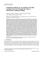
individuals in Phillipsburg, NJ, USA (Lioy et al. 1995). The full data set is presented in Figure 1.2 1
.
The first order data reduction combines all personal exposures for each day into daily frequency
distributions. This is the time series of the frequency distributions of personal exposures. It
preserves the time series data of the population, but all personal time series data are lost, thus losing the
data that relate to longer or shorter term individual health effects.
Such a database can be used for identifying the days in which given exposure limits are exceeded within
the population, and the daily percentages of the population exceeding such limits. For air pollutants,
which do not have significant indoor sources, the time series of ambient air pollution levels measured at
fixed air quality monitoring sites could be used as an approximation of the time series of the mean or
median personal exposures, but the exposure frequency distributions around these daily means must be
obtained from other information sources.


0
50
100
150
200
250
300
DAY 1 DAY 2 DAY 3 DAY 4 DAY 5 DAY 6 DAY 7 DAY 8 DAY 9 DAY 10 DAY 11 DAY 12 DAY 13 DAY 14
µg/m3

Figure 1.2 1. Personal PM
10
exposures (in Δ g/m
3
) of 14 individuals in 14 days in Phillipsburg, NJ
(Lioy et al. 1990).

A time series of frequency distributions of personal exposures in the THEES data is presented in Figure
1.2 2.
The time series of the frequency distributions of personal exposures can be combined over time to form
the second order, namely the frequency distribution of the (daily) personal exposures. Then, all
time series data are lost.
Second order frequency distribution of personal exposures shows the percentages of the daily personal
exposures in the whole population exceeding selected limits. It does not show, how these exceedances
are distributed between different individuals and times. Because the data are considerably reduced, the
frequency distribution of the personal exposures allows direct graphical and statistical comparisons of
different exposure data sets, e.g. comparison of the exposures of the suburban with downtown residents,
or residents of different cities. Data sets for frequency distributions of personal exposures have been
produced in a number of air pollution exposure studies of representative population samples, however,
in only three studies, THEES (Lioy et al. 1990), LiiLa (Alm et al. 1994, 1998), Jansen et al. (1998),
have the exposures of the same individuals been measured repeatedly to allow for estimation of the first
order time series of the frequency distributions of personal exposures.

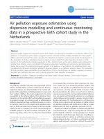
The second order frequency distribution of the personal exposures in the THEES data is presented in
Figure 1.2 3.

Figure 1.2 3. Cumulative frequency distribution of 24 h personal PM
10
exposures, together with
ambient air and indoor air PM
10
levels (in μg/m
3
) of 14 individuals in Phillipsburg, NJ
(Lioy et al. 1990).

If the frequency distribution of the personal exposures needs to be further reduced, it can be presented as
the mean or median of the (daily) personal exposures. This can be accompanied with additional
statistics, such as arithmetic or geometric standard deviation, minimum, maximum, etc. The frequency
distribution data are now lost or reduced to a number, but on the other hand, an increased number of
exposure data sets can be presented in a single table or histogram, e.g. comparison of several population
subgroups in several cities. If mean personal exposure to ambient air concentration ratios have been
determined for a representative population sample, the mean daily population exposures for a similar
population in a similar environment can be estimated from similarly acquired ambient air quality data.
The mean of the daily PM
10
exposures in the THEES study was 75 μg/m
3
, with a standard deviation of

44 μg/m
3
.
The total human exposure to air pollutants is the sum of the exposures in different locations and times.
People are exposed to outdoor air contaminants in the outdoor, indoor and transportation environments,
of which the indoor environment is the major component of the total exposure, because an
overwhelming proportion of time is spent indoors. Table 1.2-1.
presents, the range of misclassification
which could result from using outdoor air concentration as an estimate for personal exposure. It is
assumed that 85% of the time is spent indoors, 15% outdoors. The presence or absence of some
common indoor sources is also considered.




Table 1.2 1. Human exposure at home for different pollutants (Ackermann et al., 1997)

Pollutants Indoor Indoor Outdoor Actual Assigned Ratio
(μg/m
3
) source concentr. concentr. exposure exposure actual/assigned

NO
2
12.5 25 14.37 25 0.57
NO
2
gas. apply. 50 25 46.25 25 1.85
PM 15 30 17.25 30 0.57
PM tobacco 60 30 55.50 30 1.85

O
3
10 50 16 50 0.32


According to Table 1.2 1, individuals without gas appliances would have about half, with gas
appliances almost double the estimated NO
2
exposure, and very few people would actually be at the
estimated exposure level. The case of particulate matter (PM) exposures of smokers and non-smokers is
quite similar. For ozone or photochemical oxidants, with no indoor sources, the actual exposure of
everybody is much lower than the estimated exposure based on ambient air.

1.2.2. Monitoring population exposure

Monitoring population exposures is done by monitoring the exposures of the individuals separately. In
case of larger populations, the monitoring must be done by using population samples.
The focus in the monitoring is usually in the high end of exposures. For such purposes the samples
should be formed so that both long term and short term exposed subpopulations are well presented in the
population sample (Georgopoulos and Lioy 1994). When the focus is on population exposure
distribution estimation, a probability sample of the population is essential. This can be achieved locally
with a simple single stage random draw from the wanted population or in larger geographical area by a
carefully designed multistage stratified sampling procedure.

1.3. Time-Microenvironment-Activity Measurement


Air pollution exposure of an individual is a consequence of the levels of air pollutants in different
micro- and macroenvironments and the presence and activities of this individual in them. While air
pollution monitors are used to assess the former, time-microenvironment-activity monitoring techniques

are used to assess the latter. Such data is usually collected by printed personally filled time-
microenvironment- activity diaries (TMAD). However more advanced techniques are also becoming
available (Jantunen 1995). Various levels of microenvironmental differentiation have been used (see
Annex I: Table 2)
. In more recent studies this differentiation has, as a consequence of gained
experience, generally been more coarse than in earlier studies. The ECA Air Pollution Epidemiology
Programme has produced a whole report on Time Activity Patterns in Exposure Assessment (edited by
Ackerman-Liebrich et al. 1995).



1.4. Exposure Survey Designs

The basic design fundamentals of previously published studies on personal exposure or
microenvironmental air pollution levels are summarized in Annex I: Table 1. The table contains studies,
where the air pollution levels have been measured and modelled, as well as studies on measured
personal exposures and simulated exposure frequency distributions within large populations.
* Most of the studies are dealing with a single pollutant component, mostly NO
2
(10 studies)
or CO (6 studies). The remaining studies focus on pollutant mixtures, such as ETS/nicotine
(5 studies), CO/NO
2
(3 studies), VOCs (2 studies), particulate matter (2 studies), or other
and more complicated sets of pollutants (7 studies).
* Most of the studies are based on short term data representing days to weeks of exposure. 10
of the studies attempt to cover the whole year or more.
* The list contains a number of studies, where the target population is poorly defined or does
not represent major fractions of urban or national populations. Only 12 of the 34 studies are
based on probability (random) samples of large populations.

* The population sample sizes are typically small, from 10 to less than 100 for descriptive
studies that do not attempt to produce data representing large, general populations.
Population samples from 175 up to about 700 have been selected to represent general urban
populations or subpopulations, such as pre-school children in, Washington commuters, or
people living in gas range homes in L.A. Even larger populations up to several thousand
have been selected for questionnaire studies, mostly on ETS.
For designers of human exposure studies a WHO Guide (1991) recommends to begin with the
following steps:
- Define the overall objectives of this study.
- Define the target population.
- Define the pollutants and routes of exposure.
- Define the information needed.
For selecting the population sample the WHO Guide (1991) stresses the importance of obtaining a true
probability sample (which may be stratified for practical purposes) of the defined target population and
achieving a satisfactory participation rate. Satisfactory means 75% or more, which, however is often not
achieved due to the burdens that typical exposure studies impose in the participating individuals. As for
the population sample size the WHO Guide states that for a human exposure study, the total sample
should contain at least 50 individuals from the target population. Collecting exposure data from the
population sample should contain monitoring their exposures and administering diaries for time-activity
information and questionnaires about occupational classification, potential sources of pollutants,
smoking, cooking and heating fuels, travel patterns, and demographics.
Finally the WHO Guide (1991) specifically warns about four types of tempting shortcuts:
- Failure to use a proper (i.e. probability) sampling procedure
- Failure to skip the pretest (pilot)
- Failure to follow up non-participants (accept low participation rate)
- Inadequate quality control.

1.5. The Measured Air Pollutants

1.5.1. Particulate Matter; TSP, RSP, PM
10
, PM
3.5
, PM
2.5

TSP is abbreviated from Total Suspended Particulates as collected by the standard high volume sampler,
RSP is abbreviated from respirable suspended particles, usually referring to particles smaller than 3 4.5
μm in aerodynamic diameter, and mostly applied in industrial hygiene measurements. PM
10
, PM
3.5
or
PM
2.5
refer to particulate matter, where particles larger than 10, 3.5 or 2.5 μm in aerodynamic diameter
have been separated out - usually by impactor or cyclone type preseparators.

Sources

Particulate matter (PM) in the air has two different origins.
Coarse particles (>1.0 2.5 μm) are mostly produced outdoors by mechanical erosion in wind, traffic,
and materials handling - and indoors by cleaning activities by resuspension of floor dust and handling of
textiles. They contain mostly soil minerals, non-volatile organics and textile fibres. Much of the coarse
PM settles rapidly out of the air, but is also easily resuspended. The average atmospheric lifetime of
coarse PM is minutes to hours, and it can travel from metres to kilometres in the air (hundreds of
kilometres for the smallest end of the range). Therefore coarse PM levels are highly variable. In the

absence of open windows, coarse PM penetrates poorly from outdoor to indoor air, i.e. indoor air coarse
PM is mostly suspended by indoor activities.

Fine particles (< 2.5 3.5 μm) are emitted directly into the outdoor air as carbonaceous soot and
polyaromatic hydrocarbons (PAHs) by incomplete combustion processes such as diesel engines and
wood burning and into indoor air by tobacco smoking, cooking and unvented kerosene heaters. They
are also produced in the atmosphere by chemical reactions of gaseous sulfur dioxide from coal and oil
burning, diesel engines and some metal ore smelting processes, nitrogen oxides from practically all
combustion processes, most importantly road traffic, fossil fuels burning and some chemical industries,
gaseous ammonia from farming and volatile organic compounds (VOCs). Fine PM contains mostly
sulphates, nitrates, polyaromatic hydrocarbons, and elemental carbon (soot). The fine PM has very low
settling velocity in air. It sticks to any surface that it happens to hit. The average atmospheric lifetimes
of fine PM is long, days to weeks, and fine PM can travel thousands of kilometres. Fine PM penetrates
effectively through most ventilation systems, and their levels in air can be fairly uniform over areas
extending over hundreds of kilometres.

Exposure

Past Particulate Matter Exposure Studies:

On one hand the recent epidemiological findings about the public health impacts of atmospheric PM and
on the other hand the tremendous costs involved in significant reduction of the present PM levels in
most regions of the industrialized world lead to increasing demand for better information about;

• what chemical and physical characteristics of the PM are most significant for the health
consequences observed,

• what environmental, microenvironmental and individual characteristics are most significant for
personal PM exposures, and

• how much can the PM related health hazards be reduced by different control measures.



Personal exposure studies can produce answers to these questions.

In an early study on personal PM exposures of respirable PM, 37 volunteers in Watertown MA and
Steubenville OH carried personal samplers and filled time activity/diaries 12 h at the time (Dockery and
Spengler 1981). The main results of this study were that the 12 h mean personal PM exposure levels are
in reasonably good agreement with the mean outdoor respirable particulate concentrations. This
agreement could be only slightly improved by a time weighed (indoor, outdoor, smoking) model.

Sexton et al. (1984) assessed personal PM exposures of 48 volunteers in Waterbury Vermont. The
volunteers carried personal sampling pumps and filled time activity/diaries every other day for two
weeks, and their homes were also equipped with similar indoor and outdoor PM samplers. Their main
findings were that outdoor particle levels were not an important determinant of personal exposure, and
personal exposure levels were systematically higher than indoor air levels, which again were higher than
outdoor air levels. Personal 24 h average PM exposure levels were modelled with a simple time
weighed, 3 variable (intercept, exposure to smoke, work, in transit) model. Predicted exposure using
this approach agreed well with measured values, explaining 51% of the variance in personal exposure.

A total of 97 nonsmoking volunteers in two rural Tennesee communities took part in the next personal
PM exposure measurement and modelling study (Spengler et al. 1985). Personal samplers with a
cyclone preseparator that passes 50% of 3.5 μm aerodynamic diameter particles and 0% of 10 μm
particles were used. The volunteers carried the personal samplers, their homes were equipped with
indoor samplers and outdoor air levels were monitored by centrally located samplers in each of the
towns. A total of 249 personal, 266 indoor and 71 outdoor air samples are included in the analysis. The
results show that personal exposure levels of non-smoke-exposed people are higher than outdoor air
levels, and that personal exposures of smoke-exposed people are nearly twice as high as those of the
non-smoke-exposed. A regression model that includes the variables outdoor air PM, smoke exposure,

employment status, time at home, time at work, time travelling, time in public (spaces), other time, and
indoor PM explained 64% of the variance in personal exposure.

Lioy et al. (1990) used a sharp cut 10 μm personal impactor together with a 4 l/min personal pump in
Phillipsburg, NJ, to evaluate personal exposures of 14 non-smoking individuals, 8 indoor PM
10
samplers
to monitor indoor microenvironments, and 4 outdoor PM
10
samplers to monitor outdoor
microenvironments, as a part of the Total Human Environmental Exposure study (THEES). In this first
PM
10
study personal exposure levels were again higher than indoor and outdoor levels, but the latter two
levels as well as their statistical dispersions were about the same. During the two winter stagnation
episodes individual exposures and outdoor microenvironmental concentrations were strongly influenced
by the outdoor PM
10
.
The personal 4 l/min impactor sampler was also used in a much larger study to evaluate personal PM
10

exposures of the population of Riverside, CA in the PTEAM study (Wallace et al. 1991, Wallace et al.
1993, Özkaynak et al. 1993, Thomas et al. 1993, Clayton et al. 1993, Özkaynak et al. 1996). A
stratified probability sample of 178 people carried personal monitors 24 h at the time for two 12 h
samples. The particle concentrations inside and outside of the home of each of the 178 participants were
monitored with stationary PM
10
and PM
2.5

monitors, and ambient air levels were monitored at fixed sites
with high volume PM
10
samplers. Both gravimetric and elemental analyses were done. Over 95 % of
the scheduled 2900 samples were taken during the 48 days of field work and analysed with very few
equipment failures. Following each of the two 12 h monitoring periods the participants answered an
interviewer administered recall time/activity questionnaire. Daytime personal PM
10
exposure levels, as
well as the levels of nearly all particle bound elements were elevated relative to indoor and outdoor
levels. Nighttime personal exposure levels were lower than outdoor but higher than indoor levels.
Smoking, cooking, dusting and vacuuming were again found to be dominant sources for high indoor
particle loads. Reentrainment of house dust through activities not recorded in the questionnaire could


also be a source of increased exposure. PM
10
and PM
2.5
concentrations in smoking homes were
considerably greater than those measured in non-smoking homes. Correlations of personal PM
10

exposures with fixed site outdoor concentrations were low: 0.37 in the daytime and 0.54 at night.
Modelling personal exposures with a microenvironmental model partially accounted for the excess
personal exposure.

Kamens et al. (1991) looked at the particle size distributions, time variation and causes of the particle
levels, and composition of the indoor air particles in three non smoking homes in Chapel Hill NC, over
a three day period. They used indoor air samplers with 2.5 and 10 μm cut sizes, several electrical and

optical aerosol analysers to obtain particle size distributions and short term particle level variations from
0.01 to 19.4 μm. The main findings were that as an average the particulate mass was nearly evenly
distributed between the three aerodynamic particle size ranges, 37% in < 2.5μm, 26% between 2.5 and
10 μm, and 37% in > 10 μm. Aerosol size information from the automated instruments suggest that the
most significant event for generating small particles was cooking, and vacuum sweeping was the most
significant large particle generating event.

The main design features of the recent personal PM exposure studies can be found in Annex I: Table 1
.
Only one, the USEPA PTEAM study conducted in Riverside CA, is based on probability sampling from
a defined population base, and can, thus be considered to produce an exposure estimate of a larger
population than the sample itself.

Condensed Results of past Particulate Matter Exposure and Microenvironmental Studies:

The personal fine PM exposure levels and corresponding levels measured in microenvironments such as
homes, workplaces, adjacent outdoor environments and central ambient air monitoring sites are
presented in Annex I: Table 3
. The observed (geometric) mean personal exposure levels for PM
2.5

3.5

have ranged 22 - 44 μg/m
3
, home indoor 11 - 42 μg/m
3
, home outdoor 10 - 38 μg/m
3
, and central

monitoring site 18 - 33 μg/m
3
. The corresponding PM
10
levels have naturally been higher, personal
exposure 33 - 129 μg/m
3
, home indoor 22 - 78 μg/m
3
, home outdoor 18 - 83 μg/m
3
, and central
monitoring site 38 - 76 μg/m
3
.

Annex I: Table 4 summarises the impacts of certain indoor air polluting activities on personal PM
exposures and indoor concentrations. The most significant is, of course, smoking. A rough average
PM
2.5 10
level increase in smoking v.s. non-smoking environments is 30 - 40 μg/m
3
or doubling of the
non smoking level. In individual cases the impact depends strongly on the number of cigarettes
smoked, size of the room or house and the ventilation efficiency. Cooking increases PM exposures 7 -
26 μg/m
3
, unvented kerosene heaters 5 - 30 μg/m
3
, wood stoves 0 - 10 μg/m

3
, and ultrasonic humidifiers
up to 542 μg/m
3
. The humidifier case in both shocking and interesting, and probably representative to
ultrasonic humidifier type only. The PM
2.5
level increase is nearly 20 times higher than smoking, and
only by using distilled water can the level be reduced to same as smoking. These devices have been
advertised as air cleaners (sic!).

Annex I: Table 5
presents source apportionments of personal, indoor air and ambient air PM
2.5 10
,
except that no source apportionments have been published for personal PM exposures. Looking at
indoor air data Table 5 shows again that where smoking takes place, it is responsible for 24 - 71 % of
total PM mass. Cooking, where relevant, is responsible for about 25 % of indoor air PM. Wood burning
is responsible for 3 - 21 % of PM, which comes mostly from outdoor air. Soil and road dust are
responsible for 4 - 50 %, industrial and heating emissions for 10 - 38 %, and traffic emissions 5-30 % of
indoor PM. The ambient air source apportionment is different, because the roles of smoking and
cooking are very much reduced, and those of the other sources respectively increased. Most ambient air
PM
2.5 3.5
data is μg/m
3
and not % based: Secondary SO
4
=
, NO

3
-
, and NH
4
+
particles form 11 - 22 μg/m
3
of the ambient air fine particulate mass, diesel vehicles contribute 4 - 12 μg/m
3
, soil dust 1 - 23 μg/m
3
,


industrial and heating emissions 4 - 6 μg/m
3
, gasoline powered (cat) vehicles 1 - 5 μg/m
3
, woodburning
1 - 4 μg/m
3
, and cooking (not fire, but frying aerosols in LA) 2 - 3 μg/m
3
.

Exposure-Response Assessment

Particles larger than 10 μm do not penetrate deep into the lung. Particles smaller than 2.5 μm do, about
half of these particles are not exhaled, and, if insoluble, are only quite slowly removed from the lung
tissues. Particles between 2.5 and 10 μm in aerodynamic diameter show intermediate behaviour that

depends strongly on the breathing type (mouth or nose) and intensity (Bates et al. 1996).

Epidemiological Data:

Time Series Studies on Short Term Health Effects: Our knowledge about the health effects of the PM
has improved considerably since extended time series of outdoor air quality data - mostly U.S. - from
PM
10
and PM
2.5
samplers has become available for epidemiological analyses. In a study on particulate
air pollution and daily death rate in Steubenville OH (they analysed 15.000 deaths from 1974 to 1984),
Schwartz and Dockery (1992) found a 6 % increase in daily deaths when daily TSP levels increased
from 36 μg/m
3
to 209 μg/m
3
. This result has later been confirmed in new time series studies in the U.S.,
China (Xu et al. 1994), and several studies in Europe, the largest being the collaborative APHEA study
by Katsouyanni et al. (1995); in Lyon (Zmirou et al. 1996), Paris (Dab et al. 1996), Athens (Touloumi
et al. 1996), Köln (Spix and Wichmann 1996), and Milan (Vigotti et al. 1996). Combined analysis of
the APHEA data from 5 West European cities indicates a 2 % increase in daily deaths resulting from a
50 μg/m
3
increase in daily PM
10
level (Katsouyanni et al. 1997).

Schwartz and Dockery have compared their results with those of previous studies, and conclude that
there is a striking quantitative concurrence in the relative increase in total mortality versus particulates

between different studies. The APHEA study has also produced disease and hospitalisation data
(Anderson et al. 1997) which supports the findings of the mortality data, namely that existing levels of
particulate air pollutants in West European cities have a significant impact on the cardiovascular and
respiratory health of the urban populations.

Based on extensive review of the literature, WHO Air Quality Guidelines draft (6.10.1997) concludes
that a daily outdoor air PM
2.5
increase of 25 μg/m
3
increases daily total mortality by 15% and total
hospital admissions by 12.5 %, and that a daily outdoor air PM
10
increase of 50 μg/m
3
increases total
mortality by 15 ( 4 %), hospital admissions by 4.2 ( 1.6 %), cough by 23 % and asthma medication need
by 17 %.
Time series studies leave one significant question open, namely, do air pollutants just synchronise
inevitable deaths to a small extent (harvesting), or do they also significantly reduce the life expectancies
of affected individuals and populations?
Studies on Long Term Health Effects: In the first cohort study on the relationship between annual
average pollution levels and adjusted mortality-rate ratios in a cohort of 8.000 adults in six cities
followed over 14-16 years, Dockery et al. (1993) found, after controlling for gender, age, smoking,
education level, and occupational exposure, that all pollutant levels (TSP, PM
2.5
, particulate sulphate,
aerosol acidity, and SO
2
) with the exception of O

3
were associated with increasing mortality. However,
the association was strongest for PM
2.5
. An increase in the annual average level of PM
2.5
from 10 to 30
μg/m
3
was associated with an increase of total mortality by 26 %, lung and heart disease mortality by 37
%, but all other causes of death were unrelated to air pollution.

In a larger cohort study on the associations between the PM
2.5
levels and adjusted mortality rate (50
cities, 295.000 individuals), Pope et al. (1995) find that an increase of the annual average PM
2.5
by 24.5
μg/m
3
is associated with a 17 % increase in total mortality and 31 % increase in lung and heart disease
mortality.



In a U.S. study on the association of the death rate among 3.8 million babies 1 12 months of age with
outdoor air PM
10
levels during the first 2 months after birth shows that compared to the low exposure
group (PM

10
< 31  8 μg/m
3
), in the high exposure group (PM
10
> 45  5 μg/m
3
) 10 % more babies died, 26
% more from sudden infant death syndrome, and 40 % more from respiratory causes (Woodruff et al.
1997).

Concluding from the three cohort studies, typical urban outdoor air levels of PM
10
and PM
2.5
appear to
increase long term death rate, i.e. reduce life expectancy. This increase is consistent between different
studies, and seems to affect at least babies and adults. These observed increases in the long term death
rates cannot be explained by acute effects of air pol
lution, but rather relate to increased morbidity that results in earlier deaths
This is also confirmed by studies which address long-term effects of air pollution on morbidity or
physiologic measures such as lung function which strongly predict survival. In the Seventh Day
Adventists Cohort Study, the incidence of chronic bronchitis increased with long-term ambient
particulate levels (Abbey et al., 1991). In the cross-sectional semi-individual (Künzli and Tager,1997 )
studies SAPALDIA and SCARPOL, lung function and morbidity of adults and children correlated with
the long-term average ambient particulate exposure levels (Ackermann-Liebrich et al.,1997 ), (Schindler
et al.,1998 ), (Braun-Fahrländer, et al.,1997 ).

The recent studies of Dockery, Schwartz, Pope and others have led to serious discussion about the needs
to considerably reduce the levels of particulate air pollutants in urban air, and to revise the particulate

ambient air quality standards (Friedlander and Lippmann 1994).

Toxicological Data:

Currently understood toxic mechanisms of individual harmful compounds or their combinations in the
PM can hardly explain the observed mortality increases. The total mass of PM
2.5
particles inhaled into
the lung during a full year, assuming 30 μg/m
3
, is in the order of 1 mg. Indeed, this fact indicates that if
the observed health effects of the atmospheric PM are real they may not depend on the specific chemical
components of the PM. However, there are new, yet unpublished data on animal tests, which support
the epidemiological findings (Godleski et al. 1997). Healthy dogs and compromised dogs with induced
bronchitis and induced coronary heart disease, have been exposed to relatively clean urban air, in which
the fine PM fraction has been concentrated by an order of magnitude (by a series of virtual impactors).
Healthy dogs were not harmed, but when dogs with a cardiovascular or/and bronchial precondition
were exposed similarly, significant short term mortality was observed.

Assuming that the considerable fraction of urban dwellers, who live with asthma, chronic bronchitis or
coronary heart disease, do not differ significantly from these dogs, the test results indicate that the safety
margin in the present day urban air fine particle levels and air quality guidelines is very small or
nonexistent. The epidemiological studies point to exactly same conclusion.

A hypothesis by Seaton et al. (1995) suggests that ultrafine particles [mostly generated by atmospheric
chemistry and physics of gaseous and vapour phase pollutants] are able to provoke alveolar inflamation,
with release of mediators capable, in susceptible individuals, of causing exacerbations of lung disease
and of increasing blood coagulability. The authors suggest that this hypothesis be tested
epidemiologically and with animal experiments.

Indoor Air Particles?

All the available epidemiological data is based on relating PM levels measured at fixed urban outdoor
air monitoring sites to long or short term mortality and morbidity data of populations or cohorts. How


do these findings relate to the health risks of indoor air particles? Individual exposures to PM (see also
Annex I: Tables 3., 4. and 5.) can be divided to e.g. outdoor air PM (measured by most urban
monitoring sites), outdoor microenvironmental or near field PM (most importantly traffic exhaust
particles on busy streets), outdoor air particles that have penetrated indoors (ventilation air, open doors
and windows, and air leaks), particles generated by indoor activities (cooking, heating, environmental
tobacco smoke, etc.), and intentional personal exposures (smoking). In average, non-smoking
individuals appear to acquire roughly one half of their PM exposures from outdoor air particles - note,
mostly in indoor environments - and the other half from indoor and personal sources.

The near field and personal PM sources have typically a much stronger immediate impact on personal
PM exposure levels than the outdoor air PM levels. However, outdoor air PM, especially the long lived
and effectively penetrating fine PM, forms the large scale background on which the impacts of the near
field, indoor and personal PM sources are added on. It has been argued, as a justification to the time
series studies, and also shown (Jansen et al. 1998) that although the outdoor air PM level may be a poor
predictor of personal PM exposure, the day to day difference in outdoor PM level is a better predictor of
the day to day difference of the population (or group) PM exposure.

The question - can the risk estimates, based on the statistical association of population mortality and
morbidity with outdoor air PM levels, be used to estimate the health risks of exposure to PM indoors -
remains still unanswered. If the health effects of fine PM are mostly independent of the
origin/composition of the particles, as some epidemiological studies seem to indicate, then indeed the
risks of the indoor fine PM should be assessable on the basis of the outdoor air PM based
epidemiological studies. If the health effects of fine PM do depend on their origin/composition, as
toxicological plausibility seems to require, then the health effects of indoor PM cannot be directly

assessed on the basis of the outdoor air PM based epidemiological studies. This problem, however, is
lager in principle than in the praxis: Most of the individuals that are affected by elevated outdoor air PM
levels are anyway exposed indoors. In the absence of smoking, outdoor air provides 50 60% of the
indoor air particles.

Conclusions of Health Effects:

There are sufficient reasons to assume that the fine PM in urban outdoor (and indoor) air is hazardous to
public health even at the presently common relatively low concentrations. We do not know yet (i) what
characteristics make the particles harmful, although combustion generated particles are the most
suspected, (ii) what characteristics make individuals more susceptible, although individuals
compromised by cardiovascular or respiratory diseases are the most likely targets, or (iii) what
biological mechanisms are responsible for the observed acute and long term morbidity and mortality
increase, although inflammation is the most suspected.
The U.S. cohort studies on long term health effects suggest that a 10 μg/m
3
increase in the long term
mean PM
2.5
level increases total death rate by 7-13 %. U.S.EPA (1996) concludes in its new Air Quality
Criteria for PM that (very much abbreviated by the author);

• There is very much evidence that daily outdoor air fine PM (PM
2.5
) is significantly increasing
daily deaths and cases of disease at present concentrations (in North American cities).

• There is less, but still convincing evidence, that fine PM also reduces life expectancy.

• There is no clear evidence about what physical or chemical fine PM characteristics make it

hazardous.

• There is no indication of a threshold level, below which fine PM is harmless (if one exists, it is
below today's cleanest cities PM levels).



• Elderly individuals with cardiopulmonary diseases appear to be at highest risk, asthmatic
children may also form a susceptible group.
All present epidemiological evidence is based on outdoor ambient air pollution data. The observed
health risks of outdoor air PM result mostly from exposure to these particles in indoor environments (by
necessity - people spend 90% or more of their time indoors. However, although the risks of fine PM
from indoor sources (except smoking) are not known, this does not much affect risk assessment for
indoor fine PM, because 50 - 65 % of it comes from outdoor air/sources. Therefore if we can accept an
uncertainty factor of 2, we can apply the risk estimates from outdoor air PM to common indoor
exposures as well.

The epidemiological studies do not support any threshold level, below which PM exposure could be
considered safe to the general public. This is also the conclusion of a WHO expert group responsible for
preparing material for the new WHO Air Quality Guidelines (Draft 6.10.1997). Instead of an air quality
guideline value, the group suggests a unit risk for PM. The group concludes that:

• A 100 μg/m
3
increase in 24 h average PM
10
exposure results in a 6 8 %, PM
2.5
exposure in a
12 19 % increase in daily deaths within a population,

• a 50 μg/m
3
increase in 24 h average PM
10
exposure results in a 3 6 %, PM
2.5
exposure in about
25 % increase in total hospital admissions, and

• among asthmatics a 25 μg/m
3
increase in 24 h average PM
10
exposure results in a 8 % increase in
symptom exacerbation and bronchodilator use, and a 12 % increase in cough.

Even if a threshold level exists, it is likely to be so low that it is not relevant for outdoor or indoor air
quality management in the urban areas where majority of the population lives. The epidemiological
evidence and occupational hygiene experience suggest that the short term acute death risk of a 24 h
PM
10
level of 100 μg/m
3
is probably negligible for the healthy majority of the population, but amplified
for babies in their first year(s) of life, and for the large numbers of, particularly elderly, individuals with
and underlying cardiovascular or respiratory diseases.

A WHO, USEPA based research group has evaluated the health difference between two IPCC Climate
Change scenarios, one Business as Usual, the other Effective Fossil Fuel Reduction. From year 2000 to

2020 the difference between the former vs the latter is 8.000.000 cases of excess deaths from higher fine
PM from higher fossil fuel use alone (Working group 1997).

Sampling

PM
10
and PM
2.5
can now be sampled by personal sampling pumps using a sharp cut impactor to separate
the particles that are larger and smaller than 10 μm (or 2.5 μm) in aerodynamic diameter. These
samplers can operate up to 15 h with a single set of batteries (Buckley et al. 1991, Thomas et al. 1994).

Reponen et al. (1995) and Mirme et al. (1995) have compared the measurements of black smoke (BS) as
measured according to the OECD standard, and black carbon (BC) measured with an aethalometer
(Magee Scientific) with size fractionated particle count data measured by the Tartu University
developed Electrical Aerosol Spectrometer (12 size fractions between 0.01 um - 10 um). Both BS (r
2
=
0.91) and BC (r
2
= 0.93) data correlate very well with the PM
1.0
particle numbers (aerodynamic diameter
between 0.01 and 1.0 μm). As the BS and BC analyses are not gravimetric but optical, they require only
small samples, and can be considered as indirect but probably quite useful proxies for the PM
1.0
particle
numbers.

Continuously measuring personal PM monitors do exist, but until recently they have not bee sufficiently
sensitive for monitoring environmental particulate levels. There are, however, new instruments which
are sufficiently sensitive for urban environmental monitoring, battery powered, relatively lightweight,
and have memory capacity for hundreds of measurements. The new personal DataRAM monitor (MIE
Inc. Bedford, MA), is based on passive air sampling and forward light scattering principle. It is
sensitive for particles in the diameter range of 0.1 - 10 μm at concentrations down to 1 μg/m
3
. The TSI
DusTrack monitor (TSI, Inc. StPaul, MN) is also an optical aerosol monitor, but the analysed air flow is
pumped at 2.5 L/min. Consequently it can be equipped with a size selective inlet (e.g. PM
2.5
), but it is
also bigger and has a much higher battery consumption. All optical aerosol analysers are sensitive to
particle size distribution, the optical characteristics of the particles and atmospheric humidity, and need
therefore be calibrated for each measuring condition and aerosol type. This greatly limits the
applicability of optical aerosol monitors for personal exposure monitoring, where both the aerosol
characteristics and the ambient air conditions change while the person moves from one
microenvironment and activity to another.

1.5.2. Carbon Monoxide

Sources
CO is produced in incomplete combustion of carbonaceous fuels. In modern urban settings street traffic
is the dominant source of CO. For indoor exposures gas stoves, gas fired water heaters and other
unvented heating equipment may increase the indoor CO levels considerably from the outdoor levels -
even to acutely dangerous levels. The atmospheric lifetime of CO is estimated to be in the order of tens
of days, so within an urban airspace CO can taken as an inert, non reacting gas.

Exposure

The key design features of the CO exposure studies are summarized in
Annex I: Table 1.

Children:

Alm et al. (1994) studied personal CO exposures of preschool children in Helsinki, and in comparing
exposure frequency distributions between different subgroups, found that the whole exposure frequency
distributions were shifted upwards by gas stoves (which at that time in Helsinki burned man made town
gas), parental smoking at home, and low socioeconomic status of the parents, that the highest 5 % of the
exposure distribution was shifted upwards by commuting to and from the day care centre by car or bus
vs walk or bike, and that location of home in the downtown vs suburban region produced no visible
difference in the distribution curve. The 1 h personal exposures of the children showed no correlation
with, but the lowest 8 h exposures were well predicted by the fixed monitoring data.

Adults:

Cortese and Spengler showed already in 1976 that the frequency distribution of fixed ambient air quality
monitoring station CO data (Massachusetts) underestimate personal 1 h CO exposures during
commuting by a factor of 1.4 - 2.1. No consistent relationship was observed between personal exposure
during commuting and fixed station measurements over the entire range of values encountered. On the
other hand, measurements at fixed stations were representative of 8 h population exposure. The
personal exposures are strongly affected by individual modes of transportation. Individuals commuting
by auto are exposed to twice as high daily maximum 1 h levels than people commuting by mass transit.
Wind speed, wind direction, season and automobile age did not influence commuter exposure to CO.