combining svms with various feature selection strategies

Combining SVMs with Various Feature
Selection Strategies
Yi-Wei Chen and Chih-Jen Lin
Department of Computer Science, National Taiwan University, Taipei 106, Taiwan
Summary. This article investigates the performance of combining support vector
machines (SVM) and various feature selection strategies. Some of them are filter-
type approaches: general feature selection methods independent of SVM, and some
are wrapper-type methods: modifications of SVM which can be used to select fea-
tures. We apply these strategies while participating at NIPS 2003 Feature Selection
Challenge and rank third as a group.
1 Introduction
Support Vector Machine (SVM) (Boser et al. 1992; Cortes and Vapnik 1995) is
an effective classification method, but it does not directly obtain the feature
importance. In this article we combine SVM with various feature selection
strategies and investigate their performance. Some of them are “filters”: gen-
eral feature selection methods independent of SVM. That is, these methods
select important features first and then SVM is applied for classification. On
the other hand, some are wrapper-type methods: modifications of SVM which
choose important features as well as conduct training/testing. We apply these
strategies while participating at NIPS 2003 Feature Selection Challenge. Over-
all we rank third as a group and are the winner of one data set.
In NIPS 2003 Feature Selection Challenge, the main judging criterion is
the balanced error rate (BER). Its definition is:
BER ≡
1
2
(
# positive instances predicted wrong
# positive instances
+
# negative instances predicted wrong

# negative instances
) .
(1)
For example, assume a test data set contains 90 positive and 10 negative
instances. If all instances are predicted as positive, then BER is 50% since
the first term of (1) is 0/90 but the second is 10/10. There are other judg-
ing criteria such as the number of features and probes, but throughout the
competition we focus on how to get the smallest BER.
2 Yi-Wei Chen and Chih-Jen Lin
This article is organized as follows. In Section 2 we introduce support
vector classification. Section 3 discusses various feature selection strategies. In
Section 4, we show the experimental results during the development period of
the competition. In Section 5, the final competition results are listed. Finally,
we have discussion and conclusions in Section 6. All competition data sets are
available at />2 Support Vector Classification
Recently, support vector machines (SVMs) have been a promising tool for
data classification. Its basic idea is to map data into a high dimensional space
and find a separating hyperplane with the maximal margin. Given training
vectors x
k
∈ R
n
, k = 1, . . . , m in two classes, and a vector of labels y ∈ R
m
such that y
k
∈ {1, −1}, SVM solves a quadratic optimization problem:
min
w,b,ξ
1

2
w
T
w + C
m

k=1
ξ
k
, (2)
subject to y
k
(w
T
φ(x
k
) + b) ≥ 1 − ξ
k
,
ξ
k
≥ 0, k = 1, . . . , m,
where training data are mapped to a higher dimensional space by the function
φ, and C is a penalty parameter on the training error. For any testing instance
x, the decision function (predictor) is
f(x) = sgn

w
T
φ(x) + b


.
Practically, we need only k(x, x
′
) = φ(x)
T
φ(x
′
), the kernel function, to
train the SVM. The RBF kernel is used in our experiments:
k(x, x
′
) = exp(−γx − x
′

2
) . (3)
With the RBF kernel (3), there are two parameters to be determined in the
SVM model: C and γ. To get good generalization ability, we conduct a vali-
dation process to decide parameters. The procedure is as the following:
1. Consider a grid space of (C, γ) with log
2
C ∈ {−5, −3, . . . , 15} and log
2
γ ∈
{−15, −13, . . . , 3}.
2. For each hyperparameter pair (C, γ) in the search space, conduct 5-fold cross
validation on the training set.
3. Choose the parameter (C, γ) that leads to the lowest CV balanced error rate.
4. Use the best parameter to create a model as the predictor.

Combining SVMs with Various Feature Selection Strategies 3
3 Feature Selection Strategies
In this Section, we discuss feature selection strategies tried during the compe-
tition. We name each method to be like “A + B,” where A is a filter to select
features and B is a classifier or a wrapper. If a method is “A + B + C,” then
there are two filters A and B.
3.1 No Selection: Direct Use of SVM
The first strategy is to directly use SVM without feature selection. Thus, the
procedure in Section 2 is considered.
3.2 F-score for Feature Selection: F-score + SVM
F-score is a simple technique which measures the discrimination of two sets
of real numbers. Given training vectors x
k
, k = 1, . . . , m, if the number of
positive and negative instances are n
+
and n
−
, respectively, then the F-score
of the ith feature is defined as:
F (i) ≡

¯x
(+)
i
− ¯x
i

2
+


¯x
(−)
i
− ¯x
i

2
1
n
+
−1
n
+

k=1

x
(+)
k,i
− ¯x
(+)
i

2
+
1
n
−
−1

n
−

k=1

x
(−)
k,i
− ¯x
(−)
i

2
, (4)
where ¯x
i
, ¯x
(+)
i
, ¯x
(−)
i
are the average of the ith feature of the whole, positive,
and negative data sets, respectively; x
(+)
k,i
is the ith feature of the kth positive
instance, and x
(−)
k,i

is the ith feature of the kth negative instance. The numer-
ator indicates the discrimination between the positive and negative sets, and
the denominator indicates the one within each of the two sets. The larger the
F-score is, the more likely this feature is more discriminative. Therefore, we
use this score as a feature selection criterion.
A disadvantage of F-score is that is does not reveal mutual information
among features. Consider one simple example:
+1
−1
Both features of this data have low F-scores as in (4) the denominator (the
sum of variances of the positive and negative sets) is much larger than the
numerator.
4 Yi-Wei Chen and Chih-Jen Lin
Despite this disadvantage, F-score is simple and generally quite effec-
tive. We select features with high F-scores and then apply SVM for train-
ing/prediction. The procedure is summarized below:
1. Calculate F-score of every feature.
2. Pick some possible thresholds by human eye to cut low and high F-scores.
3. For each threshold, do the following
a) Drop features with F-score below this threshold.
b) Randomly split the training data into X
train
and X
valid
.
c) Let X
train
be the new training data. Use the SVM procedure in Section
2 to obtain a predictor; use the predictor to predict X
valid

.
d) Repeat the steps above five times, and then calculate the average valida-
tion error.
4. Choose the threshold with the lowest average validation error.
5. Drop features with F-score below the selected threshold. Then apply the SVM
procedure in Section 2.
In the above procedure, possible thresholds are identified by human eye.
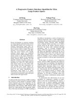
For data sets in this competition, there is a quite clear gap between high
and lower scores (see Figure 1, which will be described in Section 4). We can
automate this step by, for example, gradually adding high-F-score features,
until the validation accuracy decreases.
3.3 F-score and Random Forest for Feature Selection: F-score +
RF + SVM
Random forest (RF) is a classification method, but it also provides feature
importance (Breiman 2001). Its basic idea is as follows: A forest contains
many decision trees, each of which is constructed by instances with randomly
sampled features. The prediction is by a majority vote of decision trees. To
obtain feature importance, first we split the training sets to two parts. By
training the first and predicting the second we obtain an accuracy value. For
the jth feature, we randomly permute its values in the second set and obtain
another accuracy. The difference between the two numbers can indicate the
importance of the jth feature.
In practice, the RF code we used cannot handle too many features. Thus,
before using RF to select features, we obtain a subset of features using F-score
selection first. This approach is thus called “F-score + RF + SVM” and is
summarized below:
1. F-score
a) Consider the subset of features obtained in Section 3.2.
2. RF
a) Initialize the RF working data set to include all training instances with

the subset of features selected from Step 1. Use RF to obtain the rank
of features.
Combining SVMs with Various Feature Selection Strategies 5
b) Use RF as a predictor and conduct 5-fold CV on the working set.
c) Update the working set by removing half features which are less important
and go to Step 2b.
Stop if the number of features is small.
d) Among various feature subsets chosen above, select one with the lowest
CV error.
3. SVM
a) Apply the SVM procedure in Section 2 on the training data with the
selected features.
Note that the rank of features is obtained at Step 2a and is not updated
throughout iterations. An earlier study on using RF for feature selection is
(Svetnik et al. 2004).
3.4 Random Forest and RM-bound SVM for Feature Selection:
RF + RM-SVM
Chapelle et al. (2002) directly use SVM to conduct feature selection. They
consider the RBF kernel with feature-wise scaling factors:
k(x, x
′
) = exp

−
n

i=1
γ
i
(x

i
− x
′
i
)
2

. (5)
By minimizing an estimation of generalization errors which is a function
of γ
1
, . . . , γ
n
, we can have feature importance. Leave-one-out (loo) errors are
such an estimation and are bounded by a smoother function (Vapnik 1998):
loo ≤ 4
˜
w
2
˜
R
2
. (6)
We refer to this upper bound as the radius margin (RM) bound. Here,
˜
w
T
≡
[
w

T
√
Cξ
T
] and (w, ξ) is the optimal solution of the L2-SVM:
min
w,b,ξ
1
2
w
T
w +
C
2
m

k=1
ξ
2
k
,
under the same constraints of (2);
˜
R is the radius of the smallest sphere
containing all [
φ(x
k
)
T
e

T
k
/
√
C
] , k = 1, . . . , m, where e
k
is a zero vector except
the kth component is one.
We minimize the bound 4
˜
w
2
˜
R
2
with respect to C and γ
1
, . . . , γ
n
via a
gradient-based method. Using these parameters, an SVM model can be built
for future prediction. Therefore we call this machine an RM-bound SVM.
When the number of features is large, minimizing the RM bound is time
consuming. Thus, we apply this technique only on the problem MADELON,
which has 500 features. To further reduce the computational burden, we use
RF to pre-select important features. Thus, this method is referred to as “RF
+ RM-SVM.”
6 Yi-Wei Chen and Chih-Jen Lin
4 Experimental Results

In the experiment, we use LIBSVM
1
(Chang and Lin 2001) for SVM classi-
fication. For feature selection methods, we use the randomForest (Liaw and
Wiener 2002) package
2
in software R for RF and modify the implementation
in (Chung et al. 2003) for the RM-bound SVM
3
. Before doing experiments,
data sets are scaled. With training, validation, and testing data together, we
scale each feature to [0, 1]. Except scaling, there is no other data preprocessing.
In the development period, only labels of training sets are known. An on-
line judge returns BER of what competitors predict about validation sets, but
labels of validation sets and even information of testing sets are kept unknown.
We mainly focus on three feature selection strategies discussed in Sections
3.1-3.3: SVM, F-score + SVM, and F-score + RF + SVM. For RF + RM-
SVM, due to the large number of features, we only apply it on MADELON.
The RF procedure in Section 3.3 selects 16 features, and then RM-SVM is
used. In all experiments we focused on getting the smallest BER.
For the strategy F-score + RF + SVM, after the initial selection by F-score,
we found that RF retains all features. That is, by comparing cross-validation
BER using different subsets of features, the one with all features is the best.
Hence, F+RF+SVM is in fact the same as F+SVM for all the five data sets.
Since our validation accuracy of DOROTHEA is not as good as that by some
participants, we consider a heuristic by submitting results via the top 100,
200, and 300 features from RF. The BERs of the validation set are 0.1431,
0.1251, and 0.1498, respectively. Therefore, we consider “F-score + RF top
200 + SVM” for DOROTHEA.
Table 1 presents the BER on validation data sets by different feature

selection strategies. It shows that no method is the best on all data sets.
Table 1. Comparison of different methods during the development period: BERs
of validation sets (in percentage); bold-faced entries correspond to approaches used
to generate our final submission
Dataset ARCENE DEXTER DOROTHEA GISETTE MADELON
SVM 13.31 11.67 33.98 2.10 40.17
F+SVM 21.43 8.00 21.38 1.80 13.00
F+RF+SVM 21.43 8.00 12.51 1.80 13.00
RF+RM-SVM
4
– – – – 7.50
1
/>2
/>3
/>4
Our implementation of RF+RM-SVM is applicable to only MADELON, which
has a smaller number of features.
Combining SVMs with Various Feature Selection Strategies 7
In Table 2 we list the CV BER on the training set. Results of the first three
problems are quite different from those in Table 1. Due to the small training
sets or other reasons, CV does not accurately indicate the future performance.
Table 2. CV BER on the training set (in percentage)
Dataset ARCENE DEXTER DOROTHEA GISETTE MADELON
SVM 11.04 8.33 39.38 2.08 39.85
F+SVM 9.25 4.00 14.21 1.37 11.60
In Table 3, the first row indicates the threshold of F-score. The second
row is the number of selected features which is compared to the total number
of features in the third row. Figure 1 presents the curve of F-scores against
features.
Table 3. F-score threshold and the number of features selected in F+SVM

Dataset ARCENE DEXTER DOROTHEA GISETTE MADELON
F-score threshold 0.1 0.015 0.05 0.01 0.005
#features selected 661 209 445 913 13
#total features 10000 20000 100000 5000 500
5 Competition Results
For each data set, we submit the final result using the method that leads to
the best validation accuracy in Table 1. A comparison of competition results
(ours and winning entries) is in Tables 4 and 5.
Table 4. NIPS 2003 challenge results on December 1
st
Dec. 1
st
Our best challenge entry The winning challenge entry
Dataset Score BER AUC Feat Probe Score BER AUC Feat Probe Test
OVERALL 52.00 9.31 90.69 24.9 12.0 88.00 6.84 97.22 80.3 47.8 0.4
ARCENE 74.55 15.27 84.73 100.0 30.0 98.18 13.30 93.48 100.0 30.0 0
DEXTER 0.00 6.50 93.50 1.0 10.5 96.36 3.90 99.01 1.5 12.9 1
DOROTHEA -3.64 16.82 83.18 0.5 2.7 98.18 8.54 95.92 100.0 50.0 1
GISETTE 98.18 1.37 98.63 18.3 0.0 98.18 1.37 98.63 18.3 0.0 0
MADELON 90.91 6.61 93.39 4.8 16.7 100.00 7.17 96.95 1.6 0.0 0
For the December 1
st
submissions, we rank 1
st
on GISETTE, 3
rd
on MADE-
LON, and 5
th
on ARCENE. Overall we rank 3

rd
as a group and our best entry
8 Yi-Wei Chen and Chih-Jen Lin
0 2000 4000 6000 8000
0.00 0.15 0.30
ARCENE
Ranking of F−scores
F−score values
0 2000 4000 6000 8000
0.00 0.15 0.30
DEXTER
Ranking of F−scores
F−score values
0 20000 40000 60000 80000
0.0 0.4 0.8
DOROTHEA
Ranking of F−scores
F−score values
0 1000 2000 3000 4000 5000
0.0 0.4 0.8
GISETTE
Ranking of F−scores
F−score values
0 100 200 300 400 500
0.00 0.02 0.04
MADELON
Ranking of F−scores
F−score values
Fig. 1. Curves of F-scores against features; features with F-scores below the hori-
zontal line are dropped

Table 5. NIPS 2003 challenge results on December 8
th
Dec. 8
th
Our best challenge entry The winning challenge entry
Dataset Score BER AUC Feat Probe Score BER AUC Feat Probe Test
OVERALL 49.14 7.91 91.45 24.9 9.9 88.00 6.84 97.22 80.3 47.8 0.4
ARCENE 68.57 10.73 90.63 100.0 30.0 94.29 11.86 95.47 10.7 1.0 0
DEXTER 22.86 5.35 96.86 1.2 2.9 100.00 3.30 96.70 18.6 42.1 1
DOROTHEA 8.57 15.61 77.56 0.2 0.0 97.14 8.61 95.92 100.0 50.0 1
GISETTE 97.14 1.35 98.71 18.3 0.0 97.14 1.35 98.71 18.3 0.0 0
MADELON 71.43 7.11 92.89 3.2 0.0 94.29 7.11 96.95 1.6 0.0 1
Combining SVMs with Various Feature Selection Strategies 9
is the 6
th
, using the criterion of the organizers. For the December 8
th
submis-
sions, we rank 2
nd
as a group and our best entry is the 4
th
.
6 Discussion and Conclusions
Usually SVM suffers from a large number of features, but we find that a di-
rect use of SVM works well on GISETTE and ARCENE. After the competition,
we realize that GISETTE comes from an OCR problem MNIST (LeCun et al.
1998), which contains 784 features of gray-level values. Thus, all features are
of the same type and tend to be equally important. Our earlier experience
indicates that for such problems, SVM can handle a rather large set of fea-

tures. As the 5,000 features of GISETTE are a combination of the original 784
features, SVM may still work under the same explanation. For ARCENE, we
need further investigation to know why direct SVM performs well.
For the data set MADELON, the winner uses a kind of Bayesian SVM (Chu
et al. 2003). It is similar to RM-SVM by minimizing a function of feature-
wise scaling factors. The main difference is that RM-SVM uses an loo bound,
but Bayesian SVM derives a Bayesian evidence function. For this problem
Tables 4- 5 indicate that the two approaches achieve very similar BER. This
result seems to indicate a strong relation between the two methods. Though
they are derived from different aspects, it is worth investigating the possible
connection.
In conclusion, we have tried several feature selection strategies in this com-
petition. Most of them are independent of the classifier used. This work is a
preliminary study that for an SVM package what feature selection strategies
should be included. In the future, we would like to have a systematic compar-
ison on more data sets.
References
B. Boser, I. Guyon, and V. Vapnik. A training algorithm for optimal margin classi-
fiers. In Proceedings of the Fifth Annual Workshop on Computational Learning
Theory, pages 144–152, 1992.
Leo Breiman. Random forests. Machine Learning, 45(1):5–32, 2001. URL citeseer.
nj.nec.com/breiman01random.html.
Chih-Chung Chang and Chih-Jen Lin. LIBSVM: a library for support vector
machines, 2001. Software available at />libsvm.
O. Chapelle, V. Vapnik, O. Bousquet, and S. Mukherjee. Choosing multiple param-
eters for support vector machines. Machine Learning, 46:131–159, 2002.
W. Chu, S.S. Keerthi, and C.J. Ong. Bayesian trigonometric support vector classi-
fier. Neural Computation, 15(9):2227–2254, 2003.
Kai-Min Chung, Wei-Chun Kao, Chia-Liang Sun, Li-Lun Wang, and Chih-Jen Lin.
Radius margin bounds for support vector machines with the RBF kernel. Neural

Computation, 15:2643–2681, 2003.
10 Yi-Wei Chen and Chih-Jen Lin
C. Cortes and V. Vapnik. Support-vector network. Machine Learning, 20:273–297,
1995.
Yann LeCun, L. Bottou, Y. Bengio, and P. Haffner. Gradient-based learning applied
to document recognition. Proceedings of the IEEE, 86(11):2278–2324, November
1998. MNIST database available at />Andy Liaw and Matthew Wiener. Classification and regression by randomForest.
R News, 2/3:18–22, December 2002. URL />Rnews/Rnews_2002-3.pdf.
V. Svetnik, A. Liaw, C. Tong, and T. Wang. Application of Breiman’s random forest
to modeling structure-activity relationships of pharmaceutical molecules. In
F. Roli, J. Kittler, and T. Windeatt, editors, Proceedings of the 5th International
Workshopon Multiple Classifier Systems, Lecture Notes in Computer Science vol.
3077., pages 334–343. Springer, 2004.
Vladimir Vapnik. Statistical Learning Theory. Wiley, New York, NY, 1998.