loop-shaping robust control
Bạn đang xem bản rút gọn của tài liệu. Xem và tải ngay bản đầy đủ của tài liệu tại đây (3.69 MB, 279 trang )
Loop-shaping Robust Control
www.it-ebooks.info
Loop-shaping
Robust Control
Philippe Feyel
Series Editor
Bernard Dubuisson
www.it-ebooks.info
First published 2013 in Great Britain and the United States by ISTE Ltd and John Wiley & Sons, Inc.
Apart from any fair dealing for the purposes of research or private study, or criticism or review, as
permitted under the Copyright, Designs and Patents Act 1988, this publication may only be reproduced,
stored or transmitted, in any form or by any means, with the prior permission in writing of the publishers,
or in the case of reprographic reproduction in accordance with the terms and licenses issued by the
CLA. Enquiries concerning reproduction outside these terms should be sent to the publishers at the
undermentioned address:
ISTE Ltd John Wiley & Sons, Inc.
27-37 St George’s Road 111 River Street
London SW19 4EU Hoboken, NJ 07030
UK USA
www.iste.co.uk www.wiley.com
© ISTE Ltd 2013
The rights of Philippe Feyel to be identified as the author of this work have been asserted by him in
accordance with the Copyright, Designs and Patents Act 1988.
Library of Congress Control Number: 2013936315
British Library Cataloguing-in-Publication Data
A CIP record for this book is available from the British Library
ISBN: 978-1-84821-465-1
Printed and bound in Great Britain by CPI Group (UK) Ltd., Croydon, Surrey CR0 4YY
www.it-ebooks.info
Table of Contents
Introduction ix
Chapter 1. The Loop-shaping Approach 1
1.1.Principleofthemethod 1
1.1.1.Introduction 1
1.1.2.Sensitivity functions 1
1.1.3.Declinationofperformanceobjectives 5
1.1.4.Declinationoftherobustnessobjectives 8
1.2.Generalizedphaseandgainmargins 14
1.2.1.Phaseandgainmarginsatthemodel’soutput 14
1.2.2.Phaseandgainmarginsatthemodel’sinput: 16
1.3.Limitationsinherenttobandwidth 17
1.4.Examples 18
1.4.1.Example1:sinusoidaldisturbancerejection 18
1.4.2.Example2:referencetrackingandfrictionrejection 20
1.4.3. Example 3: issue of flexible modes and high-
frequency disturbances 25
1.4.4.Example 4: stability robustness in relation to
system uncertainties 29
1.5.Conclusion 30
Chapter 2. Loop-shaping H
Synthesis 33
2.1.Theformalismofcoprimefactorizations 33
2.1.1.Definitions 33
2.1.2.Practicalcalculationofnormalizedcoprimefactorizations 35
2.1.3.Reconstructionofatransferfunctionfromitscoprimefactors 36
www.it-ebooks.info
vi Loop-shaping Robust Control
2.1.4. Set of stabilizing controllers – Youla parameterization
of stabilizing controllers 37
2.2.Robustnessofnormalizedcoprimefactorplantdescriptions 42
2.2.1.Takingaccountofmodelinguncertainties 42
2.2.2.Stability robustness for a coprime factor plant description 43
2.2.3.Property of the equivalent “weighted mixed sensitivity” form 46
2.2.4. Expression of the synthesis criterion in “4-blocks”
equivalent form 52
2.3.Explicit solution of the problem of robust stabilization
of coprime factor plant descriptions 54
2.3.1.ExpressionoftheproblembytheYoulaparameterization 54
2.3.2.Explicitresolutionoftherobuststabilizationproblem 57
2.4. Robustness and -gap 77
2.4.1. -gap and ball of plants 77
2.4.2. Robustness results associated with the -gap 79
2.5.Loop-shapingsynthesisapproach 82
2.5.1.Motivation 82
2.5.2. Loop-shaping H
synthesis 83
2.5.3.Associatedfundamentalrobustnessresult 89
2.5.4.Phasemarginandgainmargin 89
2.5.5.4-blocksinterpretationofthemethod 90
2.5.6.Practicalimplementation 92
2.5.7.Examplesofimplementation 100
2.6.Discreteapproach 120
2.6.1.Motivations 120
2.6.2. Discrete approach to loop-shaping H
synthesis 121
2.6.3.Exampleofimplementation 127
Chapter 3. Two Degrees-of-Freedom Controllers 135
3.1. Principle 135
3.1.1.Referencetracking 135
3.1.2.Parameterizationof2-d.o.f.controllers 141
3.2.Two-stepapproach 143
3.2.1.Generalformulation 143
3.2.2.SimplificationoftheproblembytheYoulaparameterization 145
3.2.3.Extension 150
3.2.4.Settingoftheweightingfunctions 152
3.2.5.Associatedperformancerobustnessresult 154
3.3.One-stepapproach 156
3.3.1.Generalformulation 156
3.3.2.ExpressionoftheproblembyYoulaparameterization 158
3.3.3.Associatedperformancerobustnessresult 161
www.it-ebooks.info
Table of Contents vii
3.3.4. Connection between the approach and loop-shaping synthesis 163
3.4.Comparisonofthetwoapproaches 165
3.5.Example 166
3.5.1.Optimizationofanexistingcontroller(continued)–scanning 166
3.6.Compensationforameasurabledisturbanceatthemodel’soutput 174
3.6.1.Principle 174
3.6.2.Example 179
Chapter 4. Extensions and Optimizations 187
4.1. Introduction 187
4.2.Fixed-ordersynthesis 188
4.2.1. Fixed-order robust stabilization of a coprime factor
plant description 188
4.2.2.Optimizationoftheorderofthefinalcontroller 197
4.2.3.Example: fixed-order robust multivariable synthesis 214
4.3.Optimalsettingoftheweightingfunctions 220
4.3.1.Weightsettingonthebasisofafrequencyspecification 220
4.3.2. Optimal weight tuning using stochastic optimization
and metaheuristics 227
4.4. Towards a new approach to loop-shaping fixed-order
controller synthesis, etc. 242
4.4.1.Taking account of objectives of stability robustness 243
4.4.2.Takingaccountofobjectivesofperformancerobustness 244
APPENDICES 245
Appendix 1 247
Appendix 2 251
Bibliography 255
Index 259
www.it-ebooks.info
Introduction
I.1 Presentation of the book
In an increasingly competitive industrial context, an automation engineer has to
apply servo-loops in accordance with ever more complex sets of functional
specifications, associated with increasingly broad conditions of usage. In addition to
this, the product is often destined for large-scale production. Thus, the engineer has
to be able to implement a robust servo-loop on a so-called “prototype”, whilst taking
account of this broad spectrum in its entirety, at the very earliest stage of design.
An example of such a system, upon which most of the examples given in this
book are based, is a mass-produced viewfinder, for which the automation engineer
has to inertially stabilize the line of sight, whose usage conditions may be extremely
varied – indeed there are often as many potential applications as there are types of
carriers (aircraft, ships, etc.). In addition, the viewfinder is required to deliver
increasingly high-end functionalities – e.g. target tracking, guidance, etc. In order to
moderate and reduce development costs, there is a growing tendency to carry out
so-called “generic” stabilizations. This is possible only if the servo-loop designed
has a certain degree of robustness, which needs to be taken into account as an a
priori constraint on synthesis.
In the 1990s, automation engineering made a great leap forward, with the
emergence of H
∞
-based controller synthesis techniques:
– Firstly, it became possible to obey a complex set of frequency specifications by
using frequency weighting functions on exogenous inputs and on monitored signals,
and then minimizing the H
∞
transfer norm between those signals by using a
stabilizing controller whose state-space representation was explicitly formulated in
[DOY 89], inspired by a dichotomy in the solution of Riccati equations (the
so-called “γ-iteration”) and based on the following standard form:
www.it-ebooks.info
x Loop-shaping Robust Control
P(s)
K(s)
yu
z
e
Figure I.1. Standard form for control
where e represents the exogenous inputs (reference points, disturbances, etc.),
z represents the signals being monitored (error signals, commands, etc.) and
y represents the measurements used by the controller to calculate the command u.
– Secondly, the small-gain theorem gives us a necessary and sufficient condition
for the stability of the loop obtained for any uncertainty Δ(s) such that
1
()s
Δ
γ
−
∞
<
. This is stable if and only if (iff)
()
ez
Ts
γ
∞
<
, and in this
knowledge, we can take account of objectives of robustness during the synthesis
process.
T(s)
e
Δ
(s)
w
v
z
Figure I.2. Standard form for robustness analysis
Thus, with the standard approach to robust control, the complexity of controller
calculus – hitherto usually based on examination of the open loop – is now reflected
in the complexity of determining the set of relevant frequency weights, which make
a crucially important contribution to the performances of the final controller. Owing
to the difficulty in calculating these weights, the know-how that this operation
requires and the conceptual difference from conventional frequency automation
engineering, certain engineers are deterred from using the standard approach to
robust control, preferring to employ more conventional open-loop concepts.
www.it-ebooks.info
Introduction xi
However, at the same time, the world witnessed the publication of the explicit
solution to the robust stabilization of normalized coprime factor plant descriptions
[MCF 90], based on the following form.
K(s)
M(s)
-1
Δ
M
(s)
N(s)
Δ
N
(s)
v
1
v
2
w
u y
Figure I.3. Robust coprime factor plant description stabilization
– This method, which is highly attractive because of its simplicity, consists of
solving two LQG-type Riccati equations. In its 4-blocks equivalent representation, it
is a particular case of the standard H
∞
approach to robust control. Noting that we can
model the direct and complementary sensitivity functions by modeling the open-
loop response, and seeing that any loop transfer is proportional to those sensitivity
functions, it is therefore possible to model any loop transfer by working on a single
transfer – the open-loop response. This is the principle upon which loop-shaping
synthesis is founded. Drawing inspiration from frequency-shaped LQG synthesis,
we shape the singular values of the open-loop response using weighting functions on
the input and output of the system, thereby creating a loop-shape for which a
stabilizing controller can be calculated. This is the definition of H
∞
loop-shaping
synthesis.
– However, thanks to the notion of the gap metric (which expresses a distance
between two systems in mathematical terms) as well as the small-gain theorem, the
stability of the loop can be evaluated even before the controller has been explicitly
formulated.
There is a growing interest in H
∞
loop-shaping synthesis. Obviously, it is less
general than the standard H
∞
approach, because the number of degrees of freedom is
constrained by the dimensions of the system. However, the adjustment of the input
and output weighting functions on the basis of the concepts of conventional
frequency automation makes the loop-shaping technique extremely attractive and
easy to access – all the more so as it has the qualities of robustness which are
inherent to H
∞
techniques.
www.it-ebooks.info
xii Loop-shaping Robust Control
In Chapter 1, we introduce the loop-shaping approach by showing how to obtain
a specification on the open-loop response of the servo-loop from a complex
frequency specification on multiple loop transfers. Chapter 2 introduces the robust
stabilization of a normalized coprime factor plant description. Along with the notion
of the gap metric which we then introduce, it constitutes the basis for robust H
∞
loop-shaping synthesis. Chapter 3 relates to two-degrees-of-freedom controllers
(2 d.o.f controllers), and two techniques that are closely linked to H
∞
loop-shaping
synthesis are presented, thus greatly extending the possibilities for the use of the
method. Finally, Chapter 4 opens up avenues for future work: it discusses the main
drawbacks to loop-shaping synthesis, and how to solve these issues using modern
optimization techniques.
I.2. Notations and definitions
Below, we review a number of fundamental notions and notations that are
frequently employed in the various chapters of this book.
I.2.1. Linear Time-Invariant Systems (LTISs)
I.2.1.1. Representation of LTISs
An n-order linear time-invariant system with m inputs and p outputs is described
by a state-space representation defined by the following system of differential
equations:
00
() (), ( )
() () ()
dx
Axt But xt x
dt
yt Cxt Dut
=+ =
=+
where
1
:
–
()
n
x
tR∈
is the state of the system;
–
0
()
x
t
is the initial condition;
–
()
m
ut R∈
isthe system input;
–
()
p
ytR∈
is the system output;
–
nn
A R
×
∈ is the state matrix;
1 The set of real numbers is denoted as R; the set of complex numbers is denoted as C.
www.it-ebooks.info
Introduction xiii
–
nm
BR
×
∈ is the control matrix;
–
pn
CR
×
∈ is the observation matrix;
–
p
m
DR
×
∈ is the direct transfer matrix.
For a given initial condition x(t
0
), the evolution of the system’s state and its
output is given by:
() ()
0
0
0
() ( ) ( )
() () ()
t
At t At
t
x
te xt e Bud
yt Cxt Dut
τ
ττ
−−
=+
=+
The system is stable (in the sense that it has bounded input/bounded output) if
the eigenvalues of A all have a strictly negative real part, i.e. if:
[]
()
()
1,
max Re 0
i
in
A
λ
∈
<
where
()
i
A
λ
is the i
th
eigenvalue of A.
For a zero initial condition, the input/output transfer matrix of the system is
defined in Laplace form by:
()
1
()
H
sCsIABD
−
=− +
For the sake of convenience, we represent this as:
()
1
:
AB
CsI A B D
CD
−
=− +
or:
[]
()
1
,,, :ABCD C sI A B D
−
=− +
When H(∞) is bounded, H is said to be “proper”
2
. When H(∞)=0, then the
system is said to be “strictly proper”, and D = 0.
2 In the case of a SISO transfer, this means that the degree of the numerator is less than or
equal to the degree of the denominator.
www.it-ebooks.info
xiv Loop-shaping Robust Control
Finally, for the same transfer matrix, there are an infinite number of possible
state-space representations. Indeed, consider the linear transformation
nn
TR
×
∈
,
where T is invertible, such that:
x
Tx=
In this case, the initial state-space representation becomes:
1
1
() ()
() () ()
dx
TAT x t TBu t
dt
yt CT xt Dut
−
−
=+
=+
The corresponding transfer function is:
()
()
1
1
11
()CT sI TAT TBDCsIA BD Hs
−
−
−−
−+=−+=
I.2.1.2.
Controllability and observability of LTISs
The system H or the pair (A,B) is said to be controllable if, for any initial
condition x(t
0
) = x
0
, for any t
1
> 0 and for any final state x
1
, there is a piecewise
continuous command u(.) which can change the state of the system to x(t
1
) = x
1
.
We determine controllability by checking that for any value of t > t
0
, the
controllability Gramian W
c
(t) is positive definite:
0
():
T
t
ATA
c
t
Wt e BBe d
ττ
τ
=
Anequivalent condition is that the matrix
()
21n
BAB A B A B
−
must be full
row rank, i.e n.
The system H or the pair (C, A) is observable if, for any value of t
1
> 0, the initial
state x(t
0
) = x
0
can be determined by the past values of the control signal u(t) and of
the output y(t) in the interval [t
0
, t
1
].
We determine observability by checking that, for any value of t > t
0
, the
observability Gramian W
o
(t) is positive definite:
0
():
T
t
ATA
o
t
Wt e CCe d
ττ
τ
=
www.it-ebooks.info
Introduction xv
An equivalent condition is that the matrix:
2
1n
C
CA
CA
CA
−
must be full column rank, i.e. n.
I.2.1.3. Elementary operations on LTISs
Consider H, the transfer system:
()
1
:
AB
CsI A B D
CD
−
=− +
The transpose of H is defined by the system:
()
1
() :
TT
TTTTT
TT
AC
Hs BsIA C D
BD
−
=− +=
The conjugate of H is defined by the system:
()
1
*
() ( ) :
TT
TTTTT
TT
AC
Hs H s B sIA C D
BD
−
−−
=−=−− +=
If D is invertible, the inverse of H is defined by the system:
11
1
11
ABDC BD
H
DC D
−−
−
−−
−−
=
Now consider two systems H
1
and H
2
, whose respective state representations are:
11 2 2
12
11 2 2
ABAB
HH
CD C D
==
www.it-ebooks.info
xvi Loop-shaping Robust Control
The serial connection of H
1
with H
2
(or the product of H
1
by H
2
) gives us the
system:
H
2
H
1
11 2 2
12
112 2
112 12 2 2
22 12112
11212 12112
0
0
AB A B
HH
CDC D
ABC BD A B
A BBCABD
CDC DD DCCDD
=
==
The parallel connection (or addition) of H
1
to H
2
gives us the following system:
11 2 2
12
11 2 2
11
22
1212
0
0
ABAB
HH
CD CD
AB
AB
CC DD
=+
=
+
The looping of H
2
with feedback from H
1
gives us the system:
H
2
H
1
www.it-ebooks.info
Introduction xvii
()
11 1
112121121 2 121
1
111
121212 1 2 2 1 21 2 2 1 21
11 1
12 1 12 1 2 1 21
ABDR C BR C BR
IHH H BR C A BDR C BDR
RC RDC DR
−− −
−
−−−
−− −
−−
+= −
−
where
12 1 2
RIDD=+
and
21 2 1
RIDD=+
.
Many notions about linear time invariant systems are explained in [ZHO 96].
I.2.2. Singular values
I.2.2.1. Definition
The singular values of a transfer matrix H(s) of dimensions p×m are defined as
the square roots of the eigenvalues of the product of its frequency response H(jω) by
its conjugate:
()
()
()( )
(
)
()()
(
)
()
1, , min ,
TT
ii i
Hj Hj H j H j Hj
imp
σωλω ω λ ω ω
=−=−
=
The singular values are positive or null real numbers and can be classified. The
largest singular value, also called the maximum singular value, is denoted as
()
H
σ
, and the smallest, also called the minimum singular value, is denoted as
()
H
σ
.
()
()
()
()
()
()
()
()
12
H
jHj Hj Hj
σωσ ωσ ω σω
=≥ ≥≥
In the case of a monovariable system (i.e. m=p=1), the unique singular value is
equal to the gain of the frequency response:
()
()
()
()
()
H
jHjHj
σωσω ω
==
Hence, the singular values extend the notion of gain established with
monovariable systems to multivariable systems. We say that H is high-gain if
()
H
σ
is large and is low-gain if
()
H
σ
is small.
www.it-ebooks.info
xviii Loop-shaping Robust Control
I.2.2.2. Properties
In this book, we make abundant use of the following properties:
()
()
()
()
()
() ()
()
()()
()
()
()
*
111
2
2
0
2
2
0
00
if exists, 1
max
max
m
m
T
ii
xC
x
xC
x
HH
HH
HH
HH
HHHHH
Hx
H
x
Hx
H
x
σ
σσ
σσ
σα ασ
σσ σ σ
σ
σ
−−−
∈
≠
∈
≠
=⇔ =
=
=
=
==
=
=
In the case of two parallel systems, we use the following properties:
() ()
()()
()
()()
()
()()
()
1
12
2
1
12 12
2
1
12
2
max , 2 max ,
0
max ,
0
H
HH
H
H
HH HH
H
H
HH
H
σσσ
σσ σ σσ
σσσ
≤+
≤≤
=
In the case of two serial systems, an important property is:
()() ( ) ()()
()() ( ) ()()
12 12 12
12 12 12
or
iii
ii i
H
HHHHH
H
HHHHH
σσ σ σσ
σσ σ σσ
≤≤
≤≤
In particular, we shall use the following specific cases:
()() ()()()
()() ()()()
()() ()()()
()() ()()()
12 12 12
12 12 12
12 12 12
12 12 12
H
HHHHH
H
HHHHH
H
HHHHH
H
HHHHH
σσ σ σσ
σσ σ σσ
σσ σ σσ
σσ σ σσ
≤≤
≤≤
≤≤
≤≤
www.it-ebooks.info
Introduction xix
In the case of the sum of two systems, an important property is:
() () ()()()
12 12 12iii
H
HHHHH
σσ σ σσ
−≤+≤+
In particular, we shall use the following two specific cases:
() () ()() ()
() () ()() ()
12 1212
12 1212
H
HHHHH
HH HH HH
σσ σ σσ
σσ σ σσ
−≤+≤+
−≤+≤+
which lead us to:
() ()()
1I 1HHH
σσσ
−≤ + ≤ +
or indeed:
()
()
(
)
()
1
1
11
I
HH
H
σσ
σ
−
−≤ ≤ +
+
Finally, we use the following property:
() () ()
12 12
0HH HH
σσ σ
< +>
The interested reader can find further discussion about inequalities on singular
values in [MER 04].
I.2.3. Subspace RH
∞∞
and H
∞∞
norm
I.2.3.1. Definition
We use the notation L
∞
n
to represent the set of vectorial functions f(s), s ∈ C of
dimension n and bounded on the imaginary axis, i.e. which satisfy:
()
2
supffj
ω
ω
∞
=<+∞
where
2
is the Euclidean norm.
H
∞
n
is the subspace of the analytical and bounded functions of L
∞
n
in C
+
.
www.it-ebooks.info
xx Loop-shaping Robust Control
RL
∞
p×m
is the subspace of rational proper transfer matrices of dimensions p×m
with real coefficients and without pole on the imaginary axis.
RH
∞
p×m
is the subspace of rational stable
3
proper transfer matrices of dimensions
p×m with real coefficients.
For any system H ∈ RH
∞
p×m
, the H
∞
norm of H is defined by:
()
()
sup
R
HHj
ω
σω
∞
∈
=
Hence, this is the highest value of the system’s gain for the set of pulsations.
I.2.3.2. Properties
The set of properties valid for the maximum singular value is also valid for the
H
∞
norm.
In particular, in this book, we shall very frequently make use of the following
properties:
()
()
()
12 1 2
1
12
2
12 12
()() () ()
()
sup ( ) , ( )
()
sup () , () () ()
HsH s Hs H s
Hs
Hs H s
Hs
Hs H s Hs H s
∞∞∞
∞∞
∞
∞∞
∞
≤
≤
≤
Notably, this implies that:
1
2
13
24
3
4
()
()
() ()
() ()
()
()
Hs
Hs
Hs H s
Hs Hs
Hs
Hs
γ
γ
γ
γ
γ
∞
∞
∞
∞
∞
≤
≤
≤
≤
≤
Finally:
22
1
12
2
()
() ()
()
Hs
Hs H s
Hs
∞∞
∞
≤+
3 This means that they do not have a pole in C+.
www.it-ebooks.info
Introduction xxi
I.2.4. Linear fractional transformation (LFT)
I.2.4.1. Definition
Consider a complex matrix P divided as follows:
12 12
11 12
()()
21 22
p
pqq
PP
PC
PP
+×+
=∈
Consider two other complex matrices
22
qp
l
C
Δ
×
∈
and
11
qp
u
C
Δ
×
∈
.
Assuming that
()
1
22 l
IP
Δ
−
−
exists, the lower linear fractional transformation
(LFT) is defined by:
() ( )
1
1112 22 21
,
ll l l
FPPPIP P
ΔΔΔ
−
=+ −
This corresponds to the following block diagram where the matrix Δ
l
re-loops P
“from below”:
P
Δ
l
u
1
y
1
z
1
w
1
1 1 11 12 1
1 1 21 22 1
11l
zwPPw
P
yuPPu
uy
Δ
==
=
Assuming that
()
1
11 u
IP
Δ
−
−
exists, the upper LFT is defined by:
() ( )
1
22 21 11 12
,
uu u u
FPPPIP P
ΔΔΔ
−
=+ −
which corresponds to the following block diagram, where the matrix Δ
u
re-loops P
“from above”:
www.it-ebooks.info
xxii Loop-shaping Robust Control
P
Δ
u
u
2
z
2
w
2
y
2
2 2 11 12 2
2 2 21 22 2
22u
y uPPu
P
zwPPw
uy
Δ
==
=
Note also that if H
3
is invertible, then by definition:
()
()
()
()
()()
1
12 34
1
34 12
,
,
l
l
H
HQ H HQ F MQ
H
HQ H HQ F NQ
−
−
++=
++=
where:
11 1 1
13 2 13 4 3 1 3
11 1 1
334 243143
,
HHHHHH HH H
MN
HHH HHHHHH
−− − −
−− − −
−
==
−−−
I.2.4.2. Properties
A fundamental property of LFTs is that the combination of several LFTs remains
an LFT.
Consider M and Q, divided as follows:
11 12 11 12
21 22 21 22
,
MM QQ
MQ
MM QQ
==
The upper and lower LFTs are linked by the following equality:
()()
,,
uu
FM FN
ΔΔ
=
where:
22 21
12 11
00
00
MM
II
NM
MM
II
==
www.it-ebooks.info
Introduction xxiii
The inversion of an LFT is an LFT:
()
()
()
1
,,
uu
FM FN
ΔΔ
−
=
where:
11
11 12 22 21 12 22
11
22 21 22
MMMM MM
N
MM M
−−
−−
−−
=
The sum of two LFTs is an LFT:
()()()
12
,, ,
uuu
FM FQ FN
ΔΔ Δ
+=
where:
11 11
1
11 12
2
21 21 22 22
0
0
0,
0
MM
NQQ
MQMQ
Δ
Δ
Δ
==
+
The product of two LFTs is an LFT:
()()()
12
,, ,
uu u
FM FQ FN
ΔΔ Δ
=
where:
11 12 21 12 22
1
11 12
2
21 22 21 22 22
0
0,
0
MMQMQ
NMQ
MMQMQ
Δ
Δ
Δ
==
Consider G, divided as follows:
12
11112
22122
AB B
GCD D
CD D
=
www.it-ebooks.info
xxiv Loop-shaping Robust Control
The looping of two LFTs is itself an LFT:
()( )
()
()
()
()
()
12 21
,, , , , , ,
lu u ul u u
FFG FQ F FGFQ F N
ΔΔ ΔΔ Δ
==
F
u
(G,Δ
1
)
zw
F
u
(Q,Δ
2
)
where:
22212 2221 222121
12 1 2 11 12 1 22 21 12 1 21
1 12 2 22 2 12 2 21 11 12 22 1 21
1
2
1
0
0
ABQLC BLQ B BQLD
NQLCQQLDQ QLD
CDLQ C D LQ D D Q LD
Δ
Δ
Δ
++
=+
++
=
Let us conclude now with Redheffer’s theorem: if
()Ms
γ
∞
< and
1
()s
Δ
γ
−
∞
<
, then
()
(), ()
l
FMs s
Δ
γ
∞
<
.
www.it-ebooks.info
Chapter 1
The Loop-shaping Approach
1.1. Principle of the method
1.1.1. Introduction
The term “loop-shaping specification” denotes the practice of specifying the
open-loop response of a servo-loop on the basis of a specification relating to several
closed-loop transfers. The reason why we do this is that it is easier to work on a
single transfer (the open-loop response) than on a multitude of transfers (the various
loops, e.g. reference/error, disturbance/error, disturbance/control, etc.). In addition,
the internal stability of the servo-loop (i.e. the stability of all the internal loops) can
be guaranteed if the open loop response has certain characteristics (e.g. the Nyquist
locus of the open loop in relation to point -1 with a monovariable system, or
examination of the characteristic loci in the multivariable case). Hence, we can see
the advantage of synthesis methods directly based on the open loop response, the
frequency shape of which enables us to give the desired characteristics to the
different loops.
1.1.2. Sensitivity functions
To illustrate the concept, the specification of the servo-loop’s performances can
be based on the arrangement shown in Figure 1.1, which includes:
– the model’s input disturbances,
Γ
1
;
– the model’s output disturbances,
Γ
2
;
– the reference signal or measuring noise, r;
www.it-ebooks.info
2 Loop-shaping Robust Control
– the value to be controlled, y, for which we have a measurement;
– the measuring error
ε
;
– the command u created by the controller K(s), whose output disturbed by
Γ
2
is
really applied to the transfer function system H(s).
u
Γ
2
Γ
1
H(s)K(s)
r
y
ε
u' y'
Figure 1.1. General view of control system
The task of an automation engineer is then to determine a controller K(s) which,
when looped with H(s), minimizes the error
ε
at the cost of “reasonable” commands,
with the looping being subject to the external inputs r, Γ
1
and Γ
2
.
As regards the external inputs, the control and error signals are written as
1
:
11 2 2
11 2 2
11 2 2
() () () ()
() () () ()
() () () ()
ry y y
r
ru u u
ysH rsH sH s
s
H rsH sH s
us H rsH sH s
εε ε
ΓΓ
εΓΓ
ΓΓ
→→ →
→→ →
→→ →
=+ +
=+ +
=+ +
Let us now detail the different transfers involved.
1.1.2.1. Output sensitivity functions
At the system’s output, we can write:
()
()
()
() () ()
21
21
21
11 1
12
()() () () ()
() () () ()
() () () ()
() () () ()
ys s H s K rs ys
sH sHKrsHKys
IHKys s H s HKrs
ys I HK HKrs I HK H s I HK s
ΓΓ
ΓΓ
ΓΓ
ΓΓ
−− −
=− + − + −
=− − + −
+=−−+
=+ −+ −+
1 For ease of writing, the same letter-like symbols are used for temporal signals and their
Laplace transforms, and the dependency on s of the transfers is usually omitted.
www.it-ebooks.info
The Loop-shaping Approach 3
and:
() () ()
()
(
)
() ()
()()
()
() ()
() () ()
11 1
21
111
21
111
21
11 1
12
() () ()
() () . () ()
() () ()
() () . ()
() () ()
srsys
rs IHK s IHK H s IHK HKrs
I IHK HKrs IHK s IHK H s
IHK IHK HKrsIHK sIHKHs
IHK rs IHK H s IHK s
ε
ΓΓ
ΓΓ
ΓΓ
ΓΓ
−− −
−−−
−−−
−− −
=−
=++ ++ −+
=−+ ++ ++
=+ + − ++ ++
=+ ++ ++
In addition:
() () ()
11 1
12
() ()
() () ()
us K s
K
IHK rs KIHK H s KIHK s
ε
ΓΓ
−− −
=
=+ ++ ++
Denoting the output
2
sensitivity functions as follows:
11
(),()
yy
SIHK T I HK HK
−−
=+ =+
[1.1]
Thus we obtain:
12
12
12
() () () ()
() () () ()
() () () ()
yy y
yy y
yy y
ys Trs S H s S s
sSrsSH sS s
usKS r s KS H s KS s
ΓΓ
εΓΓ
ΓΓ
=− −
=+ +
=+ +
As there is no reason for the product KH to be equal to HK in the MIMO case,
we can obtain other expressions for the above signals.
1.1.2.2. Input sensitivity functions
At the system’s input, we can write:
()
()
()
() () ()
21
21
11 1
12
() () () () ()
() () () ()
() () ()
us K rs s H s us
Kr s K s KH s KHu s
I KH Kr s I KH KH s I KH K s
ΓΓ
ΓΓ
ΓΓ
−− −
=−−+−+
=+ + −
=+ ++ ++
2 That is, when we open the loop at the level of the system input.
www.it-ebooks.info