Tiêu chuẩn iso 12242 2012
Bạn đang xem bản rút gọn của tài liệu. Xem và tải ngay bản đầy đủ của tài liệu tại đây (1.42 MB, 76 trang )
ISO
12242
2012 0 01
Measurement of fluid flow in closed
conduits — Ultrasonic transit-time
meters for liquid
--`,,```,,,,````-`-`,,`,,`,`,,`---
Mesurage de débit des fluides dans les conduites fermées —
Compteurs ultrasoniques pour liquides
12242 2012
Copyright International Organization for Standardization
Provided by IHS under license with ISO
No reproduction or networking permitted without license from IHS
2012
Not for Resale
ISO 12242:2012(E)
COPYRIGHT PROTECTED DOCUMENT
2012
All rights reserved. Unless otherwise specified, no part of this publication may be reproduced or utilized in any form or by any means,
electronic or mechanical, including photocopying and microfilm, without permission in writing from either ISO at the address below or ISO’s
member body in the country of the requester.
ISO copyright office
Case postale 56 • CH-1211 Geneva 20
41 22 49 01 11
Fax + 41 22 749 09 47
Published in Switzerland
--`,,```,,,,````-`-`,,`,,`,`,,`---
Copyright International Organization for Standardization
Provided by IHS under license with ISO
No reproduction or networking permitted without license from IHS
2012
Not for Resale
ISO 12242:2012(E)
Contents
Page
Foreword ............................................................................................................................................................................. v
Introduction ....................................................................................................................................................................... vi
1
Scope ...................................................................................................................................................................... 1
2
Normative references ......................................................................................................................................... 1
3
3.1
3.2
3.3
3.4
3.5
3.6
3.7
Terms and definitions ......................................................................................................................................... 1
Quantities .............................................................................................................................................................. 1
Meter design ......................................................................................................................................................... 2
Thermodynamic conditions .............................................................................................................................. 3
Statistics ................................................................................................................................................................ 3
Calibration ............................................................................................................................................................. 5
Symbols and subscripts .................................................................................................................................... 5
Abbreviated terms ............................................................................................................................................... 7
4
4.1
4.2
4.3
4.4
4.5
4.6
4.7
Principles of measurement ............................................................................................................................... 7
Description ............................................................................................................................................................ 7
Volume flow ........................................................................................................................................................... 9
Generic description .......................................................................................................................................... 10
Time delay considerations .............................................................................................................................. 11
Refraction considerations............................................................................................................................... 14
Reynolds number .............................................................................................................................................. 15
Temperature and pressure correction ......................................................................................................... 15
5
Performance requirements ............................................................................................................................. 15
6
6.1
6.2
Uncertainty in measurement .......................................................................................................................... 16
Introduction......................................................................................................................................................... 16
Evaluation of the uncertainty components ................................................................................................ 16
7
7.1
7.2
7.3
7.4
Installation ........................................................................................................................................................... 18
General ................................................................................................................................................................. 18
Use of a prover ................................................................................................................................................... 19
Calibration in a laboratory or use of a theoretical prediction procedure........................................... 19
Additional installation effects ........................................................................................................................ 21
8
8.1
8.2
8.3
Test and calibration .......................................................................................................................................... 22
General ................................................................................................................................................................. 22
Individual testing — Use of a theoretical prediction procedure ........................................................... 22
Individual testing — Flow calibration under flowing conditions .......................................................... 23
9
9.1
9.2
9.3
9.4
9.5
9.6
Performance testing ......................................................................................................................................... 24
Introduction......................................................................................................................................................... 24
Repeatability and reproducibility .................................................................................................................. 25
Additional test for meters with externally mounted transducers......................................................... 25
Assessing the uncertainty of a meter whose performance is predicted using a theoretical
prediction procedure ........................................................................................................................................ 26
Fluid-mechanical installation conditions .................................................................................................... 26
Path failure simulation and exchange of components ........................................................................... 27
10
10.1
10.2
10.3
10.4
10.5
10.6
Meter characteristics ........................................................................................................................................ 27
Meter body, materials, and construction .................................................................................................... 27
Transducers ........................................................................................................................................................ 29
Electronics .......................................................................................................................................................... 29
Software ............................................................................................................................................................... 30
Exchange of components ............................................................................................................................... 31
Determination of density and temperature................................................................................................. 31
11
11.1
Operational practice ......................................................................................................................................... 32
General ................................................................................................................................................................. 32
--`,,```,,,,````-`-`,,`,,`,`,,`---
2012
Copyright International Organization for Standardization
Provided by IHS under license with ISO
No reproduction or networking permitted without license from IHS
Not for Resale
ISO 12242:2012(E)
11.2
11.3
11.4
11.5
Audit process ..................................................................................................................................................... 32
Operational diagnostics .................................................................................................................................. 34
Audit trail during operation; inter-comparison and inspection ............................................................ 36
Recalibration....................................................................................................................................................... 37
Annex A (normative) Temperature and pressure correction ................................................................................ 42
Annex B (informative) Effect of a change of roughness ........................................................................................ 48
Annex C (informative) Example of uncertainty calculations................................................................................. 52
Annex D (informative) Documents ............................................................................................................................... 65
--`,,```,,,,````-`-`,,`,,`,`,,`---
Bibliography ..................................................................................................................................................................... 67
Copyright International Organization for Standardization
Provided by IHS under license with ISO
No reproduction or networking permitted without license from IHS
2012
Not for Resale
ISO 12242:2012(E)
Foreword
ISO (the International Organization for Standardization) is a worldwide federation of national standards bodies
(ISO member bodies). The work of preparing International Standards is normally carried out through ISO
technical committees. Each member body interested in a subject for which a technical committee has been
established has the right to be represented on that committee. International organizations, governmental and
non-governmental, in liaison with ISO, also take part in the work. ISO collaborates closely with the International
Electrotechnical Commission (IEC) on all matters of electrotechnical standardization.
International Standards are drafted in accordance with the rules given in the ISO/IEC Directives, Part 2.
The main task of technical committees is to prepare International Standards. Draft International Standards
adopted by the technical committees are circulated to the member bodies for voting. Publication as an
International Standard requires approval by at least 75 % of the member bodies casting a vote.
Attention is drawn to the possibility that some of the elements of this document may be the subject of patent
rights. ISO shall not be held responsible for identifying any or all such patent rights.
ISO 12242 was prepared by Technical Committee ISO/TC 30, Measurement of fluid flow in closed conduits,
Subcommittee SC 5, Velocity and mass methods
--`,,```,,,,````-`-`,,`,,`,`,,`---
2012
Copyright International Organization for Standardization
Provided by IHS under license with ISO
No reproduction or networking permitted without license from IHS
Not for Resale
ISO 12242:2012(E)
Introduction
Ultrasonic meters (USMs) have become one of the accepted flow measurement technologies for a wide range
of liquid applications, including custody-transfer and allocation measurement. Ultrasonic technology has
inherent features such as no pressure loss and wide rangeability.
--`,,```,,,,````-`-`,,`,,`,`,,`---
USMs can deliver diagnostic information through which it may be possible to demonstrate that an ultrasonic
liquid flowmeter is performing in accordance with specification. Owing to the extended diagnostic capabilities,
this International Standard advocates the addition and use of automated diagnostics instead of labour-intensive
quality checks. The use of automated diagnostics makes possible a condition-based maintenance system.
Copyright International Organization for Standardization
Provided by IHS under license with ISO
No reproduction or networking permitted without license from IHS
2012
Not for Resale
INTERNATIONAL STANDARD
ISO 12242:2012(E)
Measurement of fluid flow in closed conduits — Ultrasonic
transit-time meters for liquid
1 Scope
This International Standard specifies requirements and recommendations for ultrasonic liquid flowmeters,
which utilize the transit time of ultrasonic signals to measure the flow of single-phase homogenous liquids in
There are no limits on the minimum or maximum sizes of the meter.
This International Standard specifies performance, calibration and output characteristics of ultrasonic meters
(USMs) for liquid flow measurement and deals with installation conditions. It covers installation with and without
a dedicated proving (calibration) system. It covers both in-line and clamp-on transducers (used in configurations
in which the beam is non-refracted and in those in which it is refracted). Included are both meters incorporating
meter bodies and meters with field-mounted transducers.
2 Normative references
The following referenced documents are indispensable for the application of this document. For dated
references, only the edition cited applies. For undated references, the latest edition of the referenced document
(including any amendments) applies.
ISO 4006, Measurement of fluid flow in closed conduits — Vocabulary and symbols
3 Terms and definitions
For the purposes of this document, the terms and definitions given in ISO 4006 and the following apply.
3.1
Quantities
--`,,```,,,,````-`-`,,`,,`,`,,`---
3.1.1
volume flowrate
qV
V
qV =
t
V
t
NOTE
Adapted from ISO 80000-4:2006,[42] 4-30.
3.1.2
metering pressure
absolute fluid pressure in a meter under flowing conditions to which the indicated volume of liquid is related
3.1.3
mean velocity in the meter body
v
fluid flowrate divided by the cross-sectional area of the meter body
1
2012
Copyright International Organization for Standardization
Provided by IHS under license with ISO
No reproduction or networking permitted without license from IHS
Not for Resale
ISO 12242:2012(E)
3.1.4
mean pipe velocity
vp
fluid flowrate divided by the cross-sectional area of the upstream pipe
NOTE
Where a meter has a reduced bore, the mean velocities in the upstream pipe and within the meter body itself differ.
3.1.5
path velocity
average fluid velocity on an ultrasonic path
3.1.6
Reynolds number
dimensionless parameter expressing the ratio between the inertia and viscous forces
3.1.7
pipe Reynolds number
ReD
dimensionless parameter expressing the ratio between the inertia and viscous forces in the pipe
Re D =
ρ vp D
µ
=
vp D
ν kv
ρ
is mass density;
v
is the mean pipe velocity;
D
is the pipe internal diameter;
m
is the dynamic viscosity;
ν
is the kinematic viscosity
NOTE
Where a meter has a reduced bore, it is possible also to define the throat Reynolds number, in whose definition
the mean velocity in the meter body, the meter internal diameter and the kinematic viscosity are used.
3.2
Meter design
3.2.1
meter body
pressure-containing structure of the meter
3.2.2
ultrasonic path
path travelled by an ultrasonic signal between a pair of ultrasonic transducers
3.2.3
axial path
path travelled by an ultrasonic signal either on or parallel to the axis of the pipe
3.2.4
diametrical path
ultrasonic path whereby the ultrasonic signal travels through the centre-line or long axis of the pipe
3.2.5
chordal path
ultrasonic path whereby the ultrasonic signal travels parallel to the diametrical path
--`,,```,,,,````-`-`,,`,,`,`,,`---
2
Copyright International Organization for Standardization
Provided by IHS under license with ISO
No reproduction or networking permitted without license from IHS
2012
Not for Resale
ISO 12242:2012(E)
3.2.6
field mounted
external to the pipe, attached on site, not prior to a laboratory calibration
3.3
Thermodynamic conditions
3.3.1
metering conditions
conditions, at the point of measurement, of the fluid of which the volume is to be measured
NOTE
Also known as operating conditions or actual conditions.
3.3.2
standard conditions
defined temperature and pressure conditions used in the measurement of fluid quantity so that the standard
volume is the volume that would be occupied by a quantity of fluid if it were at standard temperature and pressure
NOTE 1
Standard conditions may be defined by regulation or contract.
NOTE 2
Not preferred alternatives: reference conditions, base conditions, normal conditions, etc.
NOTE 3
Metering and standard conditions relate only to the volume of the liquid to be measured or indicated, and
should not be confused with rated operating conditions or reference conditions (see ISO/IEC Guide 99:2007,[44] 4.9 and
4.11), which refer to influence quantities (see ISO/IEC Guide 99:2007,[44] 2.52).
3.3.3
specified conditions
conditions of the fluid at which performance specifications of the meter are given
3.4
Statistics
3.4.1
error
measured quantity value minus a reference quantity value
[ISO/IEC Guide 99:2007,[44] 2.16]
3.4.2
repeatability (of results of measurements)
closeness of the agreement between the results of successive measurements of the same measurand carried
out under the same conditions of measurement
NOTE 1
These conditions are called repeatability conditions.
NOTE 2
Repeatability conditions include:
—
the same measurement procedure;
—
the same observer;
—
the same measuring instrument, used under the same conditions;
—
the same location;
—
repetition over a short period of time.
NOTE 3
Repeatability may be expressed quantitatively in terms of the dispersion characteristics of the results.
[ISO/IEC Guide 98-3:2008,[43] B.2.15]
--`,,```,,,,````-`-`,,`,,`,`,,`---
2012
Copyright International Organization for Standardization
Provided by IHS under license with ISO
No reproduction or networking permitted without license from IHS
Not for Resale
3
ISO 12242:2012(E)
3.4.3
reproducibility (of results of measurements)
closeness of the agreement between the results of measurements of the same measurand carried out under
changed conditions of measurement
NOTE 1
A valid statement of reproducibility requires specification of the conditions changed.
NOTE 2
The changed conditions may include:
—
principle of measurement;
—
method of measurement;
—
measuring instrument;
—
reference standard;
—
location;
NOTE 3
Reproducibility may be expressed quantitatively in terms of the dispersion characteristics of the results.
NOTE 4
Results are here usually understood to be corrected results.
[ISO/IEC Guide 98-3:2008,[43] B.2.16]
3.4.4
resolution
smallest difference between indications of a meter that can be meaningfully distinguished
3.4.5
zero flow reading
flowmeter reading when the liquid is at rest, i.e. both axial and non-axial velocity components are essentially zero
3.4.6
linearization
way of reducing the non-linearity of an ultrasonic meter, by applying correction factors
--`,,```,,,,````-`-`,,`,,`,`,,`---
NOTE
The linearization can be applied in the electronics of the meter or in a flow computer connected to the USM.
The correction can be, for example, piece-wise linearization or polynomial linearization.
3.4.7
uncertainty (of measurement)
parameter, associated with the result of a measurement, that characterizes the dispersion of the values that
could reasonably be attributed to the measurand
NOTE 1
The parameter may be, for example, a standard deviation (or a given multiple of it), or the half-width of an
interval having a stated level of confidence.
NOTE 2
Uncertainty of measurement comprises, in general, many components. Some of these components may be
evaluated from the statistical distribution of the results of series of measurements and can be characterized by experimental
standard deviations. The other components, which can also be characterized by standard deviations, are evaluated from
assumed probability distributions based on experience or other information.
NOTE 3
It is understood that the result of the measurement is the best estimate of the value of the measurand, and
that all components of uncertainty, including those arising from systematic effects, such as components associated with
corrections and reference standards, contribute to the dispersion.
[ISO/IEC Guide 98-3:2008,[43] B.2.18]
4
Copyright International Organization for Standardization
Provided by IHS under license with ISO
No reproduction or networking permitted without license from IHS
2012
Not for Resale
ISO 12242:2012(E)
3.4.8
standard uncertainty
u
uncertainty of the result of a measurement expressed as a standard deviation
[ISO/IEC Guide 98-3:2008,[43] 2.3.1]
3.4.9
expanded uncertainty
U
quantity defining an interval about the result of a measurement that may be expected to encompass a large
fraction of the distribution of values that could reasonably be attributed to the measurand
[ISO/IEC Guide 98-3:2008,[43] 2.3.5]
NOTE 1
The large fraction is normally 95 % and is generally associated with a coverage factor k = 2
NOTE 2
The expanded uncertainty is often referred to as the uncertainty.
3.4.10
coverage factor
numerical factor used as a multiplier of the standard uncertainty in order to obtain an expanded uncertainty
Adapted from ISO/IEC Guide 98-3:2008,[43] 2.3.6.
NOTE
3.5
Calibration
3.5.1
flow calibration
calibration in which fluid flows through the meter
3.5.2
theoretical prediction procedure
procedure by which the performance of a meter is theoretically predicted, without liquid flowing through the meter
3.5.3
performance testing
testing of a representative sample of meters to determine, for example, reproducibility and installation
requirements for meters geometrically similar to themselves
3.6
Symbols and subscripts
--`,,```,,,,````-`-`,,`,,`,`,,`---
The symbols and subscripts used in this International Standard are given in Tables 1 and 2.
5
2012
Copyright International Organization for Standardization
Provided by IHS under license with ISO
No reproduction or networking permitted without license from IHS
Not for Resale
ISO 12242:2012(E)
Table 1 — Symbols
Quantity
Symbol
Dimensionsa
SI unit
Cross-sectional area of meter body
A
2
Speed of sound in fluid
c
−1
Internal diameter of the meter body
d
Internal pipe diameter
D
Young’s modulus
E
Function of path velocities
f
1
i,j,n
1
Calibration factor
K
1
Body end correction factor
K
Path-geometry factor
K
Velocity profile correction factor
K
1
Body style correction factor
K
1
Minimum distance to a specified upstream flow disturbance
l
Integers (1,2,3, …)
2
m/s
ML−1 −2
Pa
1
−1
or m/s
l
Path length
p
Volume flowrate
qV
Internal pipe radius
r
ML−1 −2
3 −1
Pa
3/s
R
External pipe radius
Red
1
Pipe Reynolds number
ReD
1
Percentage maximum deviation in measured flowrate due to upstream
fittings
S
1
Absolute temperature of the liquid
T
Transit time
t
Time delay
t0
Mean axial fluid velocity in the meter body
v
−1
m/s
Mean axial fluid velocity on ultrasonic path, i
vi
−1
m/s
Mean axial fluid velocity in the upstream pipe
v
−1
m/s
Transducer axial separation
X
Thermal expansion coefficient
α
Θ−1
−1
Pipe wall thickness
δ
Dynamic viscosity
m
--`,,```,,,,````-`-`,,`,,`,`,,`---
Throat Reynolds number
ν
Kinematic viscosity
Θ
ML−1 −1
2 −1
ML−3
Pa s
2 /s
kg/m3
Density of the liquid
ρ
Poisson’s ratio
s
1
Angle between ultrasonic path and pipe axis
φ
rad
a
M ≡ mass; L ≡
≡
Θ ≡ temperature.
Non-refracting configuration.
Refracting configuration.
6
Copyright International Organization for Standardization
Provided by IHS under license with ISO
No reproduction or networking permitted without license from IHS
2012
Not for Resale
ISO 12242:2012(E)
Table 2 — Subscripts
Subscript
Meaning
cal
under calibration conditions
meas
measured (uncorrected)
under operational conditions
actual (corrected)
3.7
Abbreviated terms
AGC
automatic gain control
factory acceptance test
MSOS
measured speed of sound
signal to noise ratio
USM
ultrasonic meter
USMP
USM package, including meter tubes, flow conditioner, flow computer and thermowell
4 Principles of measurement
4.1
Description
The ultrasonic transit-time flowmeter is a sampling device that measures discrete path velocities using one
or more pairs of transducers. Each pair of transducers is located a known distance, l , apart such that one is
upstream of the other (see Figure 1). The upstream and downstream transducers send and receive pulses of
ultrasound alternately, referred to as contra-propagating transmission, and the times of arrival are used in the
calculation of average axial velocity, v. At any given instant, the difference between the apparent speed of sound
in a moving liquid and the speed of sound in that same liquid at rest is directly proportional to the instantaneous
velocity of the liquid. As a consequence, a measure of the average axial velocity of the liquid along a path can
be obtained by transmitting an ultrasonic signal along the path in both directions and subsequently measuring
the transit time difference.
The volume flowrate of a liquid flowing in a completely filled closed conduit is defined as the average velocity
of the liquid over a cross-section multiplied by the area of the cross-section. Thus, by measuring the average
velocity of a liquid along one or more ultrasonic paths (i.e. lines, not the area) and combining the measurements
with knowledge of the cross-sectional area and the velocity profile over the cross-section, it is possible to
obtain an estimate of the volume flowrate of the liquid in the conduit.
--`,,```,,,,````-`-`,,`,,`,`,,`---
7
2012
Copyright International Organization for Standardization
Provided by IHS under license with ISO
No reproduction or networking permitted without license from IHS
Not for Resale
ISO 12242:2012(E)
Figure 1 — Measurement principle
Several techniques can be used to obtain a measure of the average effective speed of propagation of an
ultrasonic signal in a moving liquid in order to determine the average axial flow velocity along an ultrasonic path
line. However, the normal technique applied in modern USMs is the direct time differential technique.
The basis of this technique is the measurement of the transit time of ultrasonic signals as they propagate
between a transmitter and a receiver. The velocity of propagation of the ultrasonic signal is the sum of the
speed of sound, c, and the flow velocity in the direction of propagation. Therefore the transit time upstream and
downstream can be expressed as:
lp
t fl _ up/dn ≈
∫
l =0
1
.dl
c + vl • n
1
c
is the speed of sound in the fluid;
n
is the unit normal vector to the wave front;
vl
is the flow velocity vector at location, l, on the path l .
NOTE
This is correct whether the transmitter is upstream or downstream.
With the assumptions that the flow velocity is in the axial direction only and that vi << c, where vi is the mean
axial flow velocity on ultrasonic path line i, then the upstream and downstream transit times can be written as
t fl_up =
t fl_dn =
lp
2
c − v i cos φ
lp
(3)
c + v i cos φ
Rearranging terms and solving for vi
1
t fl_dn
8
−
1
t fl_up
=
t fl_up − t fl_dn
t fl_upt fl_dn
=
2v i cos φ
lp
4
--`,,```,,,,````-`-`,,`,,`,`,,`---
Copyright International Organization for Standardization
Provided by IHS under license with ISO
No reproduction or networking permitted without license from IHS
2012
Not for Resale
ISO 12242:2012(E)
lp
vi =
∆t
2cos φ t fl_upt fl_dn
l
is the distance between the transducers;
Δt
is the difference in transit times;
φ
is the angle of inclination of the ultrasonic signal with respect to the axial direction of the flow.
(5)
The speed of sound can be calculated as follows:
1
+
--`,,```,,,,````-`-`,,`,,`,`,,`---
t fl_dn
c=
4.2
1
t fl_up
=
t fl_up + t fl_dn
t fl_upt fl_dn
(
l p t fl_up + t fl_dn
=
2c
lp
(6)
)
t fl_upt fl_dn
2
Volume flow
The individual path velocity measurements are combined by a mathematical function to yield an estimate of the
mean velocity in the meter body:
v
f v1, ..., vn)
(8)
n is the total number of paths.
Owing to variations in path configuration and different proprietary approaches of solving Formula (8), even for
a given number of paths, the exact form of f v1, ..., vn) can vary.
The relationship between the mean pipe velocity and the measured path velocities depends on the flow profile.
In fully developed flow, the flow profile depends only on the Reynolds number and the pipe roughness.
One possible solution is to calculate the mean velocity as a weighted sum of the path velocities and to apply a
velocity profile factor, K , to compensate for profile changes. The value of K is calculated by an algorithm that
takes into account flow regime (laminar, transitional, and turbulent), as well as other process variables, as required.
v = Kp
n
∑ wi vi
9
i =1
The volume flowrate, qV, is given by:
qV
Av
v
is the estimate of the mean pipe velocity;
A
is the cross-sectional area of the measurement section.
10
Note that increasing n may reduce the uncertainty associated with flow profile variations.
9
2012
Copyright International Organization for Standardization
Provided by IHS under license with ISO
No reproduction or networking permitted without license from IHS
Not for Resale
ISO 12242:2012(E)
4.3
Generic description
4.3.1
General
This sub-clause is a generic description of USMs for liquids. It recognizes the scope for variation within
commercial designs and the potential for new developments. For the purpose of description, USMs are
considered to consist of several components, namely:
a)
transducers;
b)
meter body with ultrasonic path configuration;
c)
electronic data processing and presentation unit.
NOTE
4.3.2
In a meter with externally mounted transducers, the meter body is the pipe to which the transducers are fixed.
Transducers
Transducers are the transmitters and receivers of the ultrasonic signal. They can be supplied in various forms.
Typically they comprise a piezoelectric element with electrode connections and a supporting mechanical
structure with which the process connection is made.
Typical arrangements are shown in Figures 2 and 3. To measure the axial velocity, the transducer transmits
ultrasonic waves at a non-perpendicular angle to the meter body axis in the direction of a second transducer or
reflection point in the meter body interior. There are two methods of mounting the transducers:
a)
external to the pressure-retaining boundary;
b)
internal to the pressure-retaining boundary.
The beam of the USM may be
1)
refracted;
2)
non-refracted.
Figure 2 — Non-refracted configuration
10
Copyright International Organization for Standardization
Provided by IHS under license with ISO
No reproduction or networking permitted without license from IHS
--`,,```,,,,````-`-`,,`,,`,`,,`---
2012
Not for Resale
ISO 12242:2012(E)
Figure 3 — Refracted configuration with an external mount
If the transducers are external to the pipe wall boundary, then the beam is always refracted; this configuration is
typically referred to as clamp-on or field mounted. The geometry of a refracted beam is a function of, among other
things, the liquid sound velocity (and thus temperature). The beam geometry determines the optimal transducer
position. If the transducers are not placed at their optimal position, the measurement uncertainty increases.
If the transducers are internal to the pipe wall boundary, this configuration is typically referred to as in-line; the
beam is almost always non-refracted.
4.3.3
Meter body and ultrasonic path configurations
The meter body is essentially a pipe to which the transducers are attached. Temperature and pressure have an
effect on the pipe area (see 4.7 and Annex A). In a reduced-bore meter, the area of the measurement section
is smaller than that of the pipe.
USMs are available in a variety of path configurations. The numbers of measurement paths are generally
chosen based on a requirement with respect to variations in velocity distribution and required accuracy.
As well as variations in the radial position of the measurement paths in the cross-section, the path configuration
can be varied in orientation to the pipe axis. By utilizing reflection of the ultrasonic wave from the interior of the
meter body or from a fabricated reflector, the path can traverse the cross-section several times.
Some ultrasonic path types are illustrated in Figures 4 and 5. Figure 4 shows examples of single-path meters,
Figure 5 examples of multipath meters.
Velocity measurements made on multiple paths are typically less susceptible to changes in flow profile than
those made on a single path. Double traverses in a single plane are much less sensitive to non-axial velocity
components than single traverse paths. Other configurations, e.g. the triple traverse mid-radius path, may be
sensitive to non-axial components but can be used in combination to eliminate or to reduce the effects of swirl
and cross-flow. Direct paths can be single, double or crossed.
4.3.4
Time measurement
All USMs contain an electronic part that generates and receives signals and performs time measurement.
4.4
Time delay considerations
In 4.1 it is assumed that the ultrasonic signal spends all of the transit time in the fluid and that the direction of
propagation is at an angle, φ, to the pipe wall. In a real system, the measured time between the ultrasonic signal
2012
Copyright International Organization for Standardization
Provided by IHS under license with ISO
No reproduction or networking permitted without license from IHS
--`,,```,,,,````-`-`,,`,,`,`,,`---
Not for Resale
11
ISO 12242:2012(E)
leaving the transmitter and being received at the receiver includes a time delay, t0, due to intervening materials,
electronics, signal processing, cable lengths, etc.:
tme_up/dn
t fl_up/dn
t0
11
and t 0
is small compared with the
Here it is assumed that the difference between the delay times t0
transit times tme_up/dn. Any difference between t 0
and t0
results in a zero offset.
Formulae (5) and (7) then take the form
vi =
c=
lp
∆t
2 cos φ (t me_up − t 0 )(t me_dn − t 0 )
12
l p (t me_up + t me_dn − 2t 0 )
(13)
2 (t me_up − t 0 )(t me_dn − t 0 )
a) Diametrical path
b) Diametrical path, reflecting
c) Axial path
d) Complex reflecting path
--`,,```,,,,````-`-`,,`,,`,`,,`---
Figure 4 — Some Ultrasonic path types for single-path meters
12
Copyright International Organization for Standardization
Provided by IHS under license with ISO
No reproduction or networking permitted without license from IHS
2012
Not for Resale
ISO 12242:2012(E)
b) Diametrical multipath, reflecting
--`,,```,,,,````-`-`,,`,,`,`,,`---
a) Diametrical multipath
c) Chordal multipath
d) Chordal multipath, planar
e) Chordal multipath, non-planar
f) Chordal multipath, reflected chords
g) Chordal multipath, crossed chords
h) Compound multipath
Figure 5 — Some ultrasonic path types for multipath meters
13
© ISO 2012 – All rights reserved
Copyright International Organization for Standardization
Provided by IHS under license with ISO
No reproduction or networking permitted without license from IHS
Not for Resale
ISO 12242:2012(E)
4.5
Refraction considerations
It is necessary for USMs that utilize externally mounted transducer arrangements (see Figure 3) to compensate
for refraction in order to operate properly and accurately. When a sound wave passes through an interface
between two materials at oblique angles and the materials have different acoustic impedances, both reflected
and refracted waves are produced. Sound-wave refraction takes place as the sound passes from the transducer
into the pipe wall, from the pipe wall into pipe lining (if present), and from the pipe or pipe lining into the liquid. This
is due to the different velocities of the acoustic waves within these materials. With externally mounted transducer
arrangements, Formula (5) is usually rearranged into a different form, which is derived in this subclause.
With the definition of the angles according to Figure 3, Snell’s law can be expressed as Formula (14):
cos φ t cos φ w cos φ
=
=
ct
cw
c
14
c
is the speed of sound in the transducer’s coupling wedge;
c
is the speed of sound in the wall;
c
is the speed of sound in the liquid.
As a consequence, φ and l in Formulae (5) and (12) become functions of the speeds of sound, c , c , and c and
hence in general, of the temperature, pressure, and composition of the process fluid and intervening materials.
Using the assumption (already made in 4.1) that the velocity is much smaller than the speed of sound in the
fluid, the product of the transit times in the fluid measured upstream and downstream approximately equals the
square of the transit time t fl in the fluid with no flow:
∆t
∆t
∆t 2
t fl_upt fl_dn = t fl + t fl − = t fl2 −
≈ t fl2
2
2
4
(15)
Formula (5) becomes:
vi =
lp
∆t
(16)
2cos φ t fl2
The speed of sound in the fluid can be substituted for the path length and the transit time in the fluid. Then from
Formula (14) the speed of sound and angle in the coupling wedge are substituted for the speed of sound and
angle in the fluid:
vi =
lp
∆t
cos φ t fl 2t fl
=
ct
∆t
c ∆t
=
cos φ 2t fl cos φ t 2t fl
1
The sum of the transit times in the fluid measured upstream and downstream equals twice the transit time in the fluid:
vi =
ct
∆t
cos φ t t fl_up + t fl_dn
(18)
--`,,```,,,,````-`-`,,`,,`,`,,`---
Just as in 4.4 the transit times t fl_up and t fl_dn in the fluid are replaced by the measured transit times t
t
, and the delay time t0
vi =
ct
∆t
cos φ t (t me_up + t me_dn − 2t 0 )
19
Thus the measured flow velocity is not directly dependent on the speed of sound in the fluid.
14
Copyright International Organization for Standardization
Provided by IHS under license with ISO
No reproduction or networking permitted without license from IHS
,
2012
Not for Resale
ISO 12242:2012(E)
4.6
Reynolds number
The pipe Reynolds number is given by:
Re D =
v Dρ
20
µ
D
is the internal diameter of the pipe;
v
is the mean axial liquid velocity in the pipe;
ρ
is the actual density;
m
is the dynamic viscosity.
The effect of the Reynolds number on the uncertainty of a USM is discussed in 6.2.3.
4.7
Temperature and pressure correction
During flow calibration, the meter flow calibration factor is determined and applied. Any subsequent change in
pressure or temperature from that encountered during the flow calibration alters the physical dimensions of the
meter and, if not corrected for, introduces a systematic flow measurement error. In general, the temperature
and pressure during calibration are different from those encountered under operating conditions. Temperature
and pressure correction is not always necessary for process applications. For many instruments, the influence
of pressure and temperature is typically negligible compared with the total uncertainty. For high accuracy
applications (e.g. custody transfer) and extreme temperatures or pressures, this may no longer be the case.
In A.1 to A.4, a simple approach is given to allow an initial estimate to be made of the flow error caused
by temperature and pressure conditions that differ from the calibration reference condition. If this error is
significant relative to the uncertainty required for custody transfer or allocation purposes, a more detailed
assessment of flow error has to be performed as described in A.5. ISO 17089-1:2010,[41] Annex E provides an
extensive and detailed explanation of the process and readers are advised to consult that document for the
background to many of the statements made in Annex A.
5 Performance requirements
The selection of the USM depends on its required performance. There are many different applications.
The performance is normally specified in terms of uncertainty in measured volume flowrate over a working
range of Reynolds number (or flowrate). For control purposes, any value of uncertainty may be specified. For
custody-transfer measurement, users usually refer to the performance criteria described in relevant application
standards, such as those of the International Organization for Standardization (ISO), the Organisation
Internationale de Métrologie Légale (OIML), the American Petroleum Institute (API) Manual of petroleum
measurement standards, or others where uncertainty, repeatability and linearity are specified.
The uncertainty is derived in Clause 6 using the equations derived in Clause 4. Clause 7 covers installation
effects (on both the calibration and the use of the USM). Clause 8 describes calibration. Clause 9 covers the
components of uncertainty that need only be evaluated once for a design of USM. Clause 11 covers how to
deliver the performance in Clause 5 through the audit trail, and how to maintain it through the use of diagnostics
and recalibration in the field (using a prover) and in the laboratory. Clause 10 covers meter characteristics,
especially in terms of design, manufacture and markings.
--`,,```,,,,````-`-`,,`,,`,`,,`---
15
2012
Copyright International Organization for Standardization
Provided by IHS under license with ISO
No reproduction or networking permitted without license from IHS
Not for Resale
ISO 12242:2012(E)
6 Uncertainty in measurement
6.1
Introduction
Following ISO/IEC Guide 98-3:2008,[43] this analysis is based on the mathematical relationship between the
measured volume flow and all input quantities on which it depends. The standard uncertainty of each input
quantity is evaluated and the combined uncertainty is derived by propagation of uncertainty.
The volume flow measured by a USM is given by Formulae (9) and (10). When the meter is calibrated, a
calibration factor K is included. Thus the volume flow is:
n
∑ wi vi
qV = KK p A
21
i =1
So the uncertainty depends on
a)
the uncertainty u K) in the calibration factor K
b)
the uncertainty u K
c)
the uncertainty u A) in the area of the measurement cross-section;
d)
the uncertainty u v) due to the path-velocity measurement.
K due to the velocity profile;
The evaluation of u v) is based on Formula (12) or Formula (19), as appropriate. The first factor on the right
hand side of Formula (12) and Formula (19) can be referred to as the path geometry factor, K
what transit time difference is caused by a certain path velocity and transit time. The dimensions of K
on whether Formula (12) or Formula (19) is used. The total uncertainty in the measurement of the path velocity
1)
the uncertainty u K ) in the path geometry factor;
2)
the uncertainty u t) in the time measurement;
3)
the uncertainty u t0) in the delay time compensation.
If temperature and pressure influences have to be considered, the appropriate expressions need to be included
in Formulae (12) and (21). The uncertainties of the temperature and pressure measurement are added as
additional uncertainty components.
The standard uncertainty of the flow measurement is derived from the components by propagation of uncertainty.
The level of confidence of the standard uncertainty is 68 %, assuming a normal distribution (see ISO/IEC Guide
98-3:2008,[43] 4.3.6). A coverage factor can be applied to report an expanded uncertainty with a higher level of
confidence; usually the coverage factor is k = 2, resulting in a level of confidence of approximately 95 % (see
ISO/IEC Guide 98-3:2008,[43] 6.3.3).
Examples of uncertainty calculations are given in Annex C.
6.2
Evaluation of the uncertainty components
6.2.1
Introduction
The evaluation of the uncertainty components depends, among other things, on how the meter is calibrated.
Calibration methods are
a)
theoretical prediction procedure only;
b)
flow calibration in a laboratory (no in situ use of a prover or a master meter);
--`,,```,,,,````-`-`,,`,,`,`,,`---
16
Copyright International Organization for Standardization
Provided by IHS under license with ISO
No reproduction or networking permitted without license from IHS
2012
Not for Resale
ISO 12242:2012(E)
in situ calibration, at certain time intervals, against a master meter which is itself calibrated in a flow
laboratory at certain time intervals;
in situ calibration against a prover, at certain time intervals;
in situ calibration, at certain time intervals, against a master meter which is itself calibrated against a
prover at certain time intervals.
When the meter is calibrated, a calibration factor derived from the calibration result removes some of the
sources of error. Thus, the uncertainties of all input quantities that are assumed to be constant are removed
and replaced by the uncertainty in the calibration factor which is identical to the uncertainty of the calibration.
This may apply to uncertainties u A), u K ), and u t0) when a meter is flow calibrated on the same meter body
to be installed in the field. A field calibration by means of a prover also reduces the contribution of uncertainty
u K ) that is caused by flow profile disturbances.
One way of evaluating the uncertainty of an input quantity is performance testing. This applies, for example, to the
flow-profile uncertainty caused by perturbations and to the path geometry factor with externally mounted transducers.
It is possible that some input quantities that are considered constant at calibration do not stay constant after
the meter is installed in the field. An evaluation of the long-term uncertainty, therefore, requires all components
The evaluation of the individual uncertainty components is described in 6.2.2 to 6.2.7.
NOTE
6.2.2
See also 7.4.2, 7.4.3, 7.4.4, and 7.4.1. Damage increases the uncertainty.
Uncertainty u(K) in the calibration factor (see Clause 8)
After the meter has been calibrated, the uncertainty of the calibration factor K is identical to the uncertainty of
the calibration.
If a meter is not flow-calibrated, but its performance is predicted by a theoretical prediction procedure, the
uncertainty as measured under 9.3 and 9.4 is regarded as an uncertainty in K
For calibration in the field, see 11.5.3.2.
6.2.3
Uncertainty u(Kp) in velocity profile (see Clause 7)
In the case of a fully developed turbulent flow, the effect of velocity profile on K can be estimated using the
pipe Reynolds number and the roughness of the pipe wall (see Annex B).
In the Reynolds number range between approximately 2 000 and 10 000, the flow changes from laminar to
turbulent conditions. In the region between laminar and turbulent conditions, transitional flow occurs, and the
velocity profile switches rapidly back and forth between shapes that are approximately equal to laminar and
turbulent profiles. In the process of switching back and forth, more complex velocity profiles also occur. The
Reynolds number at which transitional flow occurs and the exact nature of the transitional flow is dependent
on numerous factors, including the pipe geometry and the prevailing thermal conditions. The range of 2 000
to 10 000 is given as a general guide to the maximum and minimum limits for transitional flow, but within that
range, transition normally occupies a narrower range of Reynolds number.
The impact of transitional flow on the measurement uncertainty depends on the meter design. Meters employing
only diameter paths are very sensitive to the transition from laminar to turbulent flow, and for these meters the
value of K changes from 0,75 for laminar flow to more than 0,9 in turbulent flow. Therefore if K is incorrectly
applied because of uncertainty regarding a critical Reynolds number, large errors could be incurred. Multipath
meters that employ additional paths that are not on the diameter can reduce these effects and may also be able
to evaluate the shape of the profile and therefore detect whether the flow is laminar, transitional or turbulent.
If the USM requires a manual input to characterize the flowing liquid condition and to determine K , e.g.
liquid density and viscosity, the actual values for the density and the dynamic viscosity shall be entered in
the USM computer during calibration as well as during operation; moreover, the sensitivity of the USM to
these parameters shall be calculated so that the user can determine the need to change these parameters
--`,,```,,,,````-`-`,,`,,`,`,,`---
17
2012
Copyright International Organization for Standardization
Provided by IHS under license with ISO
No reproduction or networking permitted without license from IHS
Not for Resale
ISO 12242:2012(E)
as operating conditions change. Viscosity may also be calculated based on temperature and/or ultrasonic
measurements.
In the field, the flow profile can be disturbed because of perturbations. The value of u K
character and magnitude of the disturbance and on the sensitivity of the meter to it. The sensitivity of the meter
to flow profile disturbances can be reduced by using multiple paths. The magnitude of the disturbance can be
reduced by a flow conditioner. Flow conditioning can also have an impact on the effects of transition.
Distortion of the flow profile can occur in both laminar and turbulent conditions. In addition, thermal gradients
can occur in laminar flows, see 6.2.5.
The uncertainty due to flow profile disturbances can be estimated by performance testing (see Clause 9) with
typical perturbations [upstream fittings (bends, etc.) and upstream steps]. The performance testing evaluates
the minimum length of upstream straight pipe required for the specific meter design to achieve a specified u K
See 7.3.2, 7.3.3, 7.3.6, 7.4.2, 7.4.3, 8.3.2.4, 9.5, and 11.5.3.2.
Uncertainty u(A) in the cross-sectional area of the measurement section
6.2.4
If the meter is not flow-calibrated, it is necessary for the uncertainty of the cross-sectional area of the
measurement section to be derived from the uncertainty of the geometrical measurements. This mainly
concerns meters shipped without a meter body. The inner pipe diameter is calculated from the measured outer
pipe diameter and the wall thickness. Ovality may be significant.
The area of the measurement section is also affected by temperature and pressure (see 4.7 and Annex A).
Uncertainty u(Kg) in the path geometry factor
6.2.5
With meters shipped without a meter body, the meter factor is derived by means that depend on the specific
meter design. The uncertainty related to this process can be evaluated by performance-testing. See 9.3.
--`,,```,,,,````-`-`,,`,,`,`,,`---
Temperature has an effect on externally mounted meters because of refraction [see, for example, c
Formula (19)] and needs to be considered.
When operating in the laminar flow regime, significant thermal gradients can form in the fluid, as turbulent
mixing is absent. The resulting sound velocity gradient along the ultrasonic path causes refraction and a
departure from the assumptions used in calculating the path geometry factor. Therefore errors can occur in
laminar flows when there are differences between the fluid and ambient or pipe wall temperatures.
6.2.6
Uncertainty u(t) in the time measurement
There is uncertainty in the time measurement due to resolution, zero stability, noise and turbulence. See 8.2.2
and 11.4.2.2.
6.2.7
Uncertainty u(t0) in the delay time compensation
The time delay, t 0, is due to intervening materials, electronics, signal-processing, cable lengths, etc. The speed
of sound of the intervening materials depends on temperature. The magnitude of this effect can be calculated
and compensated for, if it is not negligible.
7 Installation
7.1
General
The requirements for installation of process meters may be substantially different from the requirements
for custody transfer meters. The purpose of this clause is to enable the user to consider the uncertainties
introduced by the installation and, if possible, to reduce them. This clause applies to calibration (Clause 8) as
well as to operation (Clause 11).
18
Copyright International Organization for Standardization
Provided by IHS under license with ISO
No reproduction or networking permitted without license from IHS
2012
Not for Resale
ISO 12242:2012(E)
In terms of installation effects there are two options:
a)
use of a prover in the field;
b)
calibration in a laboratory.
The items in 7.4 shall be considered for both options.
7.2
Use of a prover
If a prover (or a master meter calibrated in situ against a prover) is used to calibrate the USM, then the effects
of upstream bends are compensated for by the calibration. Changes in flowrate or viscosity may have an effect.
Upstream flow conditions that change after the use of the prover (e.g. a filter or flow conditioner becoming
partially blocked or opening different parallel meter tubes in a header) may also have an effect.
7.3
7.3.1
Calibration in a laboratory or use of a theoretical prediction procedure
General
If the USM is calibrated in a laboratory, then the effect of any difference between the installation at calibration
and that on site shall be considered (see Clause 9).
If the performance of the USM is predicted using a theoretical prediction procedure, then the effect of any
difference between the installation used for the tests in 9.4 and the installation on site shall be considered.
If a master meter is calibrated in a laboratory and used to calibrate the USM, then the effects of installation on
the master meter (rather than the USM) shall be considered.
7.3.2
Upstream and downstream straight pipe length requirements
--`,,```,,,,````-`-`,,`,,`,`,,`---
Various combinations of upstream fittings, valves, bends, and lengths of straight pipe can produce velocity
profile distortions at the meter inlet that may result in flowrate measurement errors. The magnitude of the
meter error depends on the type and severity of the flow distortion and on the sensitivity of the meter design
to this distortion. This error may be reduced by increasing the length of upstream straight pipes or by using
flow conditioners. Alternatively, carrying out flow calibrations in situ or under conditions similar to metering
conditions compensates for this error. Research work on installation effects is ongoing; so the installationdesigner should consult the USM manufacturer to review the latest test results and evaluate how a specific
USM design may be affected by the upstream piping configuration of the planned installation. In order to
achieve the desired meter performance, it may be necessary for the installation designer to alter the original
piping configuration or to include a flow conditioner as part of the meter run.
Typical upstream piping conditions (operating conditions) like bends, headers, T-joints, flow conditioners,
filtration equipment, diameter changes (steps, expanders, reducers), and valves introduce swirl, an asymmetric
flow profile, a flat flow profile, a peaked flow profile or combinations of these. A length of straight pipe upstream
of the USM or USMP can reduce these effects.
The minimum length of straight upstream pipe, l , between an upstream fitting and the USM is the minimum
length such that for that length and for all longer lengths the calibration factor of the USM is within a specified
value S % of the value in a long straight pipe. The value of S is small where the overall uncertainty is low. The
value of l
is different for different upstream piping configurations, and can only be determined using a set of
reference standards. Determination of l
for a standard set of upstream piping configurations is a major task
during performance testing; see Clause 9. The manufacturer shall supply l
for each perturbation defined in
9.5 for at least one value of S. Determination of l
of an upstream piping configuration for which l
is not yet
known is the responsibility of the user.
The recommended minimum length of straight downstream pipe is 3D
The important difference in 7.1 is the difference between the performance in the field and that at calibration. If
l
upstream, but the calibration is not undertaken in a sufficiently long straight pipe, the
19
2012
Copyright International Organization for Standardization
Provided by IHS under license with ISO
No reproduction or networking permitted without license from IHS
Not for Resale