investment analysis and portfolio management

Contents in Brief

Chapter 1 - The Investment Setting
Chapter 2 - The Asset Allocation Decision
Chapter 3 - Selecting Investments in a Global Market
Chapter 4 - Organization and Functioning of Securities Markets
Chapter 5 - Security Market Indicator Series
Chapter 6 - Efficient Capital Markets
Chapter 7 - An Introduction to Portfolio Management
Chapter 8 - An Introduction to Asset Pricing Models
Chapter 9 - Multifactor Models of Risk and Return
Chapter 10 - Analysis of Financial Statements
Chapter 11 - An Introduction to Security Valuation
Chapter 12 - Macroeconomic and Market Analysis: The Global Asset
Allocation Decision
Chapter 13 - Stock Market Analysis
Chapter 14 - Industry Analysis
Chapter 15 - Company Analysis and Stock Valuation
Chapter 16 - Technical Analysis
Chapter 17 - Equity Portfolio Management Strategies
Chapter 18 - Bond Fundamentals
Chapter 19 - The Analysis and Valuation of Bonds
Chapter 20 - Bond Portfolio Management Strategies
Chapter 21 - An Introduction to Derivative Markets and Securities
Chapter 22 - Forward and Futures Contracts
Chapter 23 - Option Contracts
Chapter 24 - Swap Contracts, Convertible Securities, and Other Embedded Derivatives
Chapter 25 - Professional Asset Management
Chapter 26 - Evaluation of Portfolio Performance

Appendix A - How to Become a CFA Charterholder

Appendix B - AIMR Code of Ethics and Standards of Professional Conduct
Appendix C - Interest Tables
Appendix D - Standard Normal Probabilities

Glossary
4
Chapter
1
The Investment
Setting
After you read this chapter, you should be able to answer the following questions:
➤ Why do individuals invest?
➤ What is an investment?
➤ How do investors measure the rate of return on an investment?
➤ How do investors measure the risk related to alternative investments?
➤ What factors contribute to the rates of return that investors require on alternative
investments?
➤ What macroeconomic and microeconomic factors contribute to changes in the required
rates of return for individual investments and investments in general?
This initial chapter discusses several topics basic to the subsequent chapters. We begin by
defining the term investment and discussing the returns and risks related to investments. This
leads to a presentation of how to measure the expected and historical rates of returns for an indi-
vidual asset or a portfolio of assets. In addition, we consider how to measure risk not only for an
individual investment but also for an investment that is part of a portfolio.
The third section of the chapter discusses the factors that determine the required rate of return
for an individual investment. The factors discussed are those that contribute to an asset’s total
risk. Because most investors have a portfolio of investments, it is necessary to consider how to
measure the risk of an asset when it is a part of a large portfolio of assets. The risk that prevails

when an asset is part of a diversified portfolio is referred to as its systematic risk.
The final section deals with what causes changes in an asset’s required rate of return over
time. Changes occur because of both macroeconomic events that affect all investment assets and
microeconomic events that affect the specific asset.
WHAT ISANINVESTMENT?
For most of your life, you will be earning and spending money. Rarely, though, will your current
money income exactly balance with your consumption desires. Sometimes, you may have more
money than you want to spend; at other times, you may want to purchase more than you can
afford. These imbalances will lead you either to borrow or to save to maximize the long-run ben-
efits from your income.
When current income exceeds current consumption desires, people tend to save the excess.
They can do any of several things with these savings. One possibility is to put the money under
a mattress or bury it in the backyard until some future time when consumption desires exceed
current income. When they retrieve their savings from the mattress or backyard, they have the
same amount they saved.
Another possibility is that they can give up the immediate possession of these savings for
a future larger amount of money that will be available for future consumption. This tradeoff of
present consumption for a higher level of future consumption is the reason for saving. What you
do with the savings to make them increase over time is investment.
1
Those who give up immediate possession of savings (that is, defer consumption) expect to
receive in the future a greater amount than they gave up. Conversely, those who consume more
than their current income (that is, borrow) must be willing to pay back in the future more than
they borrowed.
The rate of exchange between future consumption (future dollars) and current consumption
(current dollars) is the pure rate of interest. Both people’s willingness to pay this difference for
borrowed funds and their desire to receive a surplus on their savings give rise to an interest rate
referred to as the pure time value of money. This interest rate is established in the capital market
by a comparison of the supply of excess income available (savings) to be invested and the
demand for excess consumption (borrowing) at a given time. If you can exchange $100 of cer-

tain income today for $104 of certain income one year from today, then the pure rate of exchange
on a risk-free investment (that is, the time value of money) is said to be 4 percent (104/100 – 1).
The investor who gives up $100 today expects to consume $104 of goods and services in the
future. This assumes that the general price level in the economy stays the same. This price sta-
bility has rarely been the case during the past several decades when inflation rates have varied
from 1.1 percent in 1986 to 13.3 percent in 1979, with an average of about 5.4 percent a year
from 1970 to 2001. If investors expect a change in prices, they will require a higher rate of return
to compensate for it. For example, if an investor expects a rise in prices (that is, he or she expects
inflation) at the rate of 2 percent during the period of investment, he or she will increase the
required interest rate by 2 percent. In our example, the investor would require $106 in the future
to defer the $100 of consumption during an inflationary period (a 6 percent nominal, risk-free
interest rate will be required instead of 4 percent).
Further, if the future payment from the investment is not certain, the investor will demand an
interest rate that exceeds the pure time value of money plus the inflation rate. The uncertainty of
the payments from an investment is the investment risk. The additional return added to the nom-
inal, risk-free interest rate is called a risk premium. In our previous example, the investor would
require more than $106 one year from today to compensate for the uncertainty. As an example,
if the required amount were $110, $4, or 4 percent, would be considered a risk premium.
From our discussion, we can specify a formal definition of investment. Specifically, an investment
is the current commitment of dollars for a period of time in order to derive future payments that
will compensate the investor for (1) the time the funds are committed, (2) the expected rate of
inflation, and (3) the uncertainty of the future payments. The “investor” can be an individual, a
government, a pension fund, or a corporation. Similarly, this definition includes all types of
investments, including investments by corporations in plant and equipment and investments by
individuals in stocks, bonds, commodities, or real estate. This text emphasizes investments by
individual investors. In all cases, the investor is trading a known dollar amount today for some
expected future stream of payments that will be greater than the current outlay.
At this point, we have answered the questions about why people invest and what they want
from their investments. They invest to earn a return from savings due to their deferred con-
sumption. They want a rate of return that compensates them for the time, the expected rate of

inflation, and the uncertainty of the return. This return, the investor’s required rate of return,
is discussed throughout this book. A central question of this book is how investors select invest-
ments that will give them their required rates of return.
Investment Defined
WHAT ISANINVESTMENT? 5
1
In contrast, when current income is less than current consumption desires, people borrow to make up the difference.
Although we will discuss borrowing on several occasions, the major emphasis of this text is how to invest savings.
6 CHAPTER 1 THE INVESTMENT SETTING
The next section of this chapter describes how to measure the expected or historical rate of
return on an investment and also how to quantify the uncertainty of expected returns. You need
to understand these techniques for measuring the rate of return and the uncertainty of these
returns to evaluate the suitability of a particular investment. Although our emphasis will be on
financial assets, such as bonds and stocks, we will refer to other assets, such as art and antiques.
Chapter 3 discusses the range of financial assets and also considers some nonfinancial assets.
M
EASURES OF RETURN AND RISK
The purpose of this book is to help you understand how to choose among alternative investment
assets. This selection process requires that you estimate and evaluate the expected risk-return
trade-offs for the alternative investments available. Therefore, you must understand how to mea-
sure the rate of return and the risk involved in an investment accurately. To meet this need, in this
section we examine ways to quantify return and risk. The presentation will consider how to mea-
sure both historical and expected rates of return and risk.
We consider historical measures of return and risk because this book and other publications
provide numerous examples of historical average rates of return and risk measures for various
assets, and understanding these presentations is important. In addition, these historical results are
often used by investors when attempting to estimate the expected rates of return and risk for an
asset class.
The first measure is the historical rate of return on an individual investment over the time
period the investment is held (that is, its holding period). Next, we consider how to measure the

average historical rate of return for an individual investment over a number of time periods. The
third subsection considers the average rate of return for a portfolio of investments.
Given the measures of historical rates of return, we will present the traditional measures of
risk for a historical time series of returns (that is, the variance and standard deviation).
Following the presentation of measures of historical rates of return and risk, we turn to esti-
mating the expected rate of return for an investment. Obviously, such an estimate contains a great
deal of uncertainty, and we present measures of this uncertainty or risk.
When you are evaluating alternative investments for inclusion in your portfolio, you will often be
comparing investments with widely different prices or lives. As an example, you might want to
compare a $10 stock that pays no dividends to a stock selling for $150 that pays dividends of
$5 a year. To properly evaluate these two investments, you must accurately compare their histor-
ical rates of returns. A proper measurement of the rates of return is the purpose of this section.
When we invest, we defer current consumption in order to add to our wealth so that we can
consume more in the future. Therefore, when we talk about a return on an investment, we are
concerned with the change in wealth resulting from this investment. This change in wealth can
be either due to cash inflows, such as interest or dividends, or caused by a change in the price of
the asset (positive or negative).
If you commit $200 to an investment at the beginning of the year and you get back $220 at
the end of the year, what is your return for the period? The period during which you own an
investment is called its holding period, and the return for that period is the holding period
return (HPR). In this example, the HPR is 1.10, calculated as follows:
HPR
Ending Value of Investment
Beginning Value of Investment
=
==
$
$
.
220

200
110
Measures of
Historical Rates
of Return
➤1.1
This value will always be zero or greater—that is, it can never be a negative value. A value greater than
1.0 reflects an increase in your wealth, which means that you received a positive rate of return during
the period. A value less than 1.0 means that you suffered a decline in wealth, which indicates that you
had a negative return during the period. An HPR of zero indicates that you lost all your money.
Although HPR helps us express the change in value of an investment, investors generally eval-
uate returns in percentage terms on an annual basis. This conversion to annual percentage rates
makes it easier to directly compare alternative investments that have markedly different character-
istics. The first step in converting an HPR to an annual percentage rate is to derive a percentage
return, referred to as the holding period yield (HPY). The HPY is equal to the HPR minus 1.
➤1.2 HPY = HPR – 1
In our example:
HPY = 1.10 – 1 = 0.10
= 10%
To derive an annual HPY, you compute an annual HPR and subtract 1. Annual HPR is found by:
➤1.3 Annual HPR = HPR
1/n
where:
n
= number of years the investment is held
Consider an investment that cost $250 and is worth $350 after being held for two years:
If you experience a decline in your wealth value, the computation is as follows:
A multiple year loss over two years would be computed as follows:
HPR
Ending Value

Beginning Value
Annual HPR
Annual HPY
===
==
=
===
$
$,
.
(. ) .
.
.–. –. –.%
//
750
1 000
075
075 075
0 866
0 866 1 00 0 134 13 4
112n
HPR
Ending Value
Beginning Value
HPY
===
===
$
$
.

.–.–.–%
400
500
080
080 100 020 20
HPR
Ending Value of Investment
Beginning Value of Investment
Annual HPR
Annual HPY
==
=
=
=
=
==
=
$
$
.
.
.
.
.–.
.%
/
/
350
250
140

140
140
1 1832
1 1832 1 0 1832
18 32
1
12
n
MEASURES OF RETURN AND RISK 7
In contrast, consider an investment of $100 held for only six months that earned a return of $12:
Note that we made some implicit assumptions when converting the HPY to an annual basis. This
annualized holding period yield computation assumes a constant annual yield for each year. In the
two-year investment, we assumed an 18.32 percent rate of return each year, compounded. In the par-
tial year HPR that was annualized, we assumed that the return is compounded for the whole year.
That is, we assumed that the rate of return earned during the first part of the year is likewise earned
on the value at the end of the first six months. The 12 percent rate of return for the initial six months
compounds to 25.44 percent for the full year.
2
Because of the uncertainty of being able to earn the
same return in the future six months, institutions will typically not compound partial year results.
Remember one final point: The ending value of the investment can be the result of a positive
or negative change in price for the investment alone (for example, a stock going from $20 a share
to $22 a share), income from the investment alone, or a combination of price change and income.
Ending value includes the value of everything related to the investment.
Now that we have calculated the HPY for a single investment for a single year, we want to con-
sider mean rates of return for a single investment and for a portfolio of investments. Over a
number of years, a single investment will likely give high rates of return during some years and
low rates of return, or possibly negative rates of return, during others. Your analysis should con-
sider each of these returns, but you also want a summary figure that indicates this investment’s
typical experience, or the rate of return you should expect to receive if you owned this invest-

ment over an extended period of time. You can derive such a summary figure by computing the
mean annual rate of return for this investment over some period of time.
Alternatively, you might want to evaluate a portfolio of investments that might include simi-
lar investments (for example, all stocks or all bonds) or a combination of investments (for exam-
ple, stocks, bonds, and real estate). In this instance, you would calculate the mean rate of return
for this portfolio of investments for an individual year or for a number of years.
Single Investment Given a set of annual rates of return (HPYs) for an individual invest-
ment, there are two summary measures of return performance. The first is the arithmetic mean
return, the second the geometric mean return. To find the arithmetic mean (AM), the sum (∑)
of annual HPYs is divided by the number of years (n) as follows:
➤1.4 AM =∑HPY/n
where:
¬HPY = the sum of annual holding period yields
Computing Mean
Historical Returns
HPR
Annual HPR
Annual HPY
== =
=
=
=
==
=
$
$
.( .)
.
.
.

.–.
.%
/.
112
100
112 05
112
112
1 2544
1 2544 1 0 2544
25 44
15
2
n
8 CHAPTER 1 THE INVESTMENT SETTING
2
To check that you understand the calculations, determine the annual HPY for a three-year HPR of 1.50. (Answer:
14.47 percent.) Compute the annual HPY for a three-month HPR of 1.06. (Answer: 26.25 percent.)
An alternative computation, the geometric mean (GM), is the nth root of the product of the
HPRs for n years.
➤1.5 GM = [π HPR]
1/n
– 1
where:
o=the product of the annual holding period returns as follows:
(HPR
1
) × (HPR
2
)

(HPR
n
)
To illustrate these alternatives, consider an investment with the following data:
AM = [(0.15) + (0.20) + (–0.20)]/3
= 0.15/3
= 0.05 = 5%
GM = [(1.15) × (1.20) × (0.80)]
1/3
– 1
= (1.104)
1/3
– 1
= 1.03353 – 1
= 0.03353 = 3.353%
Investors are typically concerned with long-term performance when comparing alternative
investments. GM is considered a superior measure of the long-term mean rate of return because
it indicates the compound annual rate of return based on the ending value of the investment ver-
sus its beginning value.
3
Specifically, using the prior example, if we compounded 3.353 percent
for three years, (1.03353)
3
, we would get an ending wealth value of 1.104.
Although the arithmetic average provides a good indication of the expected rate of return for
an investment during a future individual year, it is biased upward if you are attempting to mea-
sure an asset’s long-term performance. This is obvious for a volatile security. Consider, for
example, a security that increases in price from $50 to $100 during year 1 and drops back to $50
during year 2. The annual HPYs would be:

BEGINNING ENDING
YEAR VALUE VALUE HPR HPY
1 50 100 2.00 1.00
2 100 50 0.50 –0.50
BEGINNING ENDING
Y
EAR VALUE
VALUE HPR HPY
1 100.0 115.0 1.15 0.15
2 115.0 138.0 1.20 0.20
3 138.0 110.4 0.80 –0.20
MEASURES OF RETURN AND RISK 9
3
Note that the GM is the same whether you compute the geometric mean of the individual annual holding period yields
or the annual HPY for a three-year period, comparing the ending value to the beginning value, as discussed earlier under
annual HPY for a multiperiod case.
This would give an AM rate of return of:
[(1.00) + (–0.50)]/2 = .50/2
= 0.25 = 25%
This investment brought no change in wealth and therefore no return, yet the AM rate of return
is computed to be 25 percent.
The GM rate of return would be:
(2.00 × 0.50)
1/2
– 1 = (1.00)
1/2
– 1
= 1.00 – 1 = 0%
This answer of a 0 percent rate of return accurately measures the fact that there was no change
in wealth from this investment over the two-year period.

When rates of return are the same for all years, the GM will be equal to the AM. If the rates
of return vary over the years, the GM will always be lower than the AM. The difference between
the two mean values will depend on the year-to-year changes in the rates of return. Larger annual
changes in the rates of return—that is, more volatility—will result in a greater difference
between the alternative mean values.
An awareness of both methods of computing mean rates of return is important because pub-
lished accounts of investment performance or descriptions of financial research will use both the
AM and the GM as measures of average historical returns. We will also use both throughout this
book. Currently most studies dealing with long-run historical rates of return include both AM
and GM rates of return.
A Portfolio of Investments The mean historical rate of return (HPY) for a portfolio of
investments is measured as the weighted average of the HPYs for the individual investments in
the portfolio, or the overall change in value of the original portfolio. The weights used in com-
puting the averages are the relative beginning market values for each investment; this is referred
to as dollar-weighted or value-weighted mean rate of return. This technique is demonstrated by
the examples in Exhibit 1.1. As shown, the HPY is the same (9.5 percent) whether you compute
the weighted average return using the beginning market value weights or if you compute the
overall change in the total value of the portfolio.
Although the analysis of historical performance is useful, selecting investments for your port-
folio requires you to predict the rates of return you expect to prevail. The next section discusses
how you would derive such estimates of expected rates of return. We recognize the great uncer-
tainty regarding these future expectations, and we will discuss how one measures this uncer-
tainty, which is referred to as the risk of an investment.
Risk is the uncertainty that an investment will earn its expected rate of return. In the examples
in the prior section, we examined realized historical rates of return. In contrast, an investor who
is evaluating a future investment alternative expects or anticipates a certain rate of return. The
investor might say that he or she expects the investment will provide a rate of return of 10 per-
cent, but this is actually the investor’s most likely estimate, also referred to as a point estimate.
Pressed further, the investor would probably acknowledge the uncertainty of this point estimate
return and admit the possibility that, under certain conditions, the annual rate of return on this

investment might go as low as –10 percent or as high as 25 percent. The point is, the specifica-
tion of a larger range of possible returns from an investment reflects the investor’s uncertainty
regarding what the actual return will be. Therefore, a larger range of expected returns makes the
investment riskier.
Calculating
Expected Rates
of Return
10 CHAPTER 1 T
HE INVESTMENT SETTING
An investor determines how certain the expected rate of return on an investment is by ana-
lyzing estimates of expected returns. To do this, the investor assigns probability values to all pos-
sible returns. These probability values range from zero, which means no chance of the return, to
one, which indicates complete certainty that the investment will provide the specified rate of
return. These probabilities are typically subjective estimates based on the historical performance
of the investment or similar investments modified by the investor’s expectations for the future.
As an example, an investor may know that about 30 percent of the time the rate of return on this
particular investment was 10 percent. Using this information along with future expectations
regarding the economy, one can derive an estimate of what might happen in the future.
The expected return from an investment is defined as:
➤1.6
E(R
i
) = [(P
1
)(R
1
) + (P
2
)(R
2

) + (P
3
)(R
3
) +

+ (P
n
R
n
)]
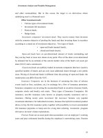
Let us begin our analysis of the effect of risk with an example of perfect certainty wherein the
investor is absolutely certain of a return of 5 percent. Exhibit 1.2 illustrates this situation.
Perfect certainty allows only one possible return, and the probability of receiving that return
is 1.0. Few investments provide certain returns. In the case of perfect certainty, there is only one
value for P
i
R
i
:
E(R
i
) = (1.0)(0.05) = 0.05
In an alternative scenario, suppose an investor believed an investment could provide several
different rates of return depending on different possible economic conditions. As an example, in
a strong economic environment with high corporate profits and little or no inflation, the investor
might expect the rate of return on common stocks during the next year to reach as high as 20 per-
cent. In contrast, if there is an economic decline with a higher-than-average rate of inflation, the
investor might expect the rate of return on common stocks during the next year to be –20 per-
cent. Finally, with no major change in the economic environment, the rate of return during the

next year would probably approach the long-run average of 10 percent.
ER P R
iii
i
n
() ()()=
=
∑
1
Expected Return Probability of Return) (Possible Return)=×
=
∑
(
i
n
1
MEASURES OF RETURN AND RISK 11
COMPUTATION OF HOLDING PERIOD YIELD FOR A PORTFOLIO
NUMBER BEGINNING BEGINNING ENDING ENDING MARKET WEIGHTED
INVESTMENT OF SHARES PRICE MARKET VALUE PRICE MARKET VALUE HPR HPY WEIGHT
a
HPY
A 100,000 $10 $ 1,000,000 $12 $ 1,200,000 1.20 20% 0.05 0.01
B 200,000 20 4,000,000 21 4,200,000 1.05 5 0.20 0.01
C 500,000 30 15,000,000 33 16,500,000 1.10 10 0.75 0.075
Total $20,000,000 $21,900,000 0.095
EXHIBIT 1.1
HPR
HPY
==

==
=
21 900 000
20 000 000
1 095
1 095 1 0 095
95
,,
,,
.
.– .
.%
a
Weights are based on beginning values.
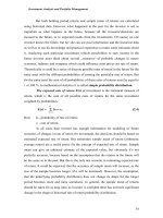
The investor might estimate probabilities for each of these economic scenarios based on past
experience and the current outlook as follows:
This set of potential outcomes can be visualized as shown in Exhibit 1.3.
The computation of the expected rate of return [E(R
i
)] is as follows:
E(R
i
) = [(0.15)(0.20)] + [(0.15)(–0.20)] + [(0.70)(0.10)]
= 0.07
Obviously, the investor is less certain about the expected return from this investment than about
the return from the prior investment with its single possible return.
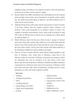
A third example is an investment with 10 possible outcomes ranging from –40 percent to
50 percent with the same probability for each rate of return. A graph of this set of expectations
would appear as shown in Exhibit 1.4.
In this case, there are numerous outcomes from a wide range of possibilities. The expected

rate of return [E(R
i
)] for this investment would be:
E(R
i
) = (0.10)(–0.40) + (0.10)(–0.30) + (0.10)(–0.20) + (0.10)(–0.10) + (0.10)(0.0)
+ (0.10)(0.10) + (0.10)(0.20) + (0.10)(0.30) + (0.10)(0.40) + (0.10)(0.50)
= (–0.04) + (–0.03) + (–0.02) + (–0.01) + (0.00) + (0.01) + (0.02) + (0.03)
+ (0.04) + (0.05)
= 0.05
RATE OF
ECONOMIC CONDITIONS PROBABILITY RETURN
Strong economy, no inflation 0.15 0.20
Weak economy, above-average inflation 0.15 –0.20
No major change in economy 0.70 0.10
12 CHAPTER 1 THE INVESTMENT SETTING
Probability
1.00
0.75
0.50
0.25
0
–.05 0.0 0.05 0.10 0.15
Rate of Return
EXHIBIT 1.2
PROBABILITY DISTRIBUTION FOR RISK-FREE INVESTMENT
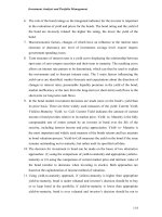
The expected rate of return for this investment is the same as the certain return discussed in
the first example; but, in this case, the investor is highly uncertain about the actual rate of return.
This would be considered a risky investment because of that uncertainty. We would anticipate
that an investor faced with the choice between this risky investment and the certain (risk-free)

case would select the certain alternative. This expectation is based on the belief that most
investors are risk averse, which means that if everything else is the same, they will select the
investment that offers greater certainty.
We have shown that we can calculate the expected rate of return and evaluate the uncertainty, or
risk, of an investment by identifying the range of possible returns from that investment and
assigning each possible return a weight based on the probability that it will occur. Although the
graphs help us visualize the dispersion of possible returns, most investors want to quantify this
Measuring the Risk
of Expected Rates
of Return
M
EASURES OF RETURN AND RISK 13
0
–0.30
Rate of Return
Probability
–0.20
–0.10
0.0 0.10
0.20
0.30
0.20
0.40
0.60
0.80
EXHIBIT 1.3
PROBABILITY DISTRIBUTION FOR RISKY INVESTMENT WITH THREE POSSIBLE
RATES OF RETURN
0
Rate of Return

Probability
0.500.400.300.200.100.0–0.10–0.20–0.30
–0.40
0.05
0.10
0.15
EXHIBIT 1.4
PROBABILITY DISTRIBUTION FOR RISKY INVESTMENT WITH 10 POSSIBLE
RATES OF RETURN
dispersion using statistical techniques. These statistical measures allow you to compare the
return and risk measures for alternative investments directly. Two possible measures of risk
(uncertainty) have received support in theoretical work on portfolio theory: the variance and the
standard deviation of the estimated distribution of expected returns.
In this section, we demonstrate how variance and standard deviation measure the dispersion
of possible rates of return around the expected rate of return. We will work with the examples
discussed earlier. The formula for variance is as follows:
➤1.7
Variance The larger the variance for an expected rate of return, the greater the dispersion of
expected returns and the greater the uncertainty, or risk, of the investment. The variance for the
perfect-certainty example would be:
Note that, in perfect certainty, there is no variance of return because there is no deviation
from expectations and, therefore, no risk or uncertainty. The variance for the second example
would be:
Standard Deviation The standard deviation is the square root of the variance:
➤1.8
For the second example, the standard deviation would be:
Therefore, when describing this example, you would contend that you expect a return of 7 per-
cent, but the standard deviation of your expectations is 11.87 percent.
A Relative Measure of Risk In some cases, an unadjusted variance or standard deviation
can be misleading. If conditions for two or more investment alternatives are not similar—that is,

σ=
==
0 0141
0 11874 11 874
.
%
Standard Deviation =
[]
=
∑
PR ER
ii i
i
n
–()
2
1
() –()
( . )( . – . ) ( . )(– . – . ) ( . )( . – . )

.
σ
2
2
1
222
015 020 007 015 020 007 070 010 007
0 010935 0 002535 0 00063
0 0141
=

[]
=++
[]
=++
[]
=
=
∑
PR ER
ii i
i
n
() –()
.(. . ) .(.)
σ
2
2
1
2
10 005 005 10 00 0
=
[]
=−==
=
∑
PR ER
ii i
i
n
Variance ( (Probability)

Possible
Return
Expected
Return
2
=
σ )
() –()
=×−




=
[]
∑
∑
=
i
n
ii i
i
n
PR ER
1
2
2
1
14 CHAPTER 1 THE INVESTMENT SETTING
if there are major differences in the expected rates of return—it is necessary to use a measure of

relative variability to indicate risk per unit of expected return. A widely used relative measure of
risk is the coefficient of variation (CV), calculated as follows:
➤1.9
The CV for the preceding example would be:
This measure of relative variability and risk is used by financial analysts to compare alterna-
tive investments with widely different rates of return and standard deviations of returns. As an
illustration, consider the following two investments:
Comparing absolute measures of risk, investment B appears to be riskier because it has a stan-
dard deviation of 7 percent versus 5 percent for investment A. In contrast, the CV figures show
that investment B has less relative variability or lower risk per unit of expected return because it
has a substantially higher expected rate of return:
To measure the risk for a series of historical rates of returns, we use the same measures as for
expected returns (variance and standard deviation) except that we consider the historical holding
period yields (HPYs) as follows:
➤1.10
where:
r
2
= the variance of the series
HPY
i
= the holding period yield during period i
E(HPY) = the expected value of the holding period yield that is equal to the arithmetic mean of
the series
n = the number of observations
σ
2
2
1
=

[]
=
∑
HPY HPY
i
i
n
En–( )/
Risk Measures for
Historical Returns
CV
CV
A
B
==
==
005
007
0 714
007
012
0 583
.
.
.
.
.
.
INVESTMENT AINVESTMENT B
Expected return 0.07 0.12

Standard deviation 0.05 0.07
CV =
=
0.11874
0.07000
1 696.
Coefficient of
Variation (CV)
Standard Deviation of Returns
Expected Rate of Return
=
=
σ
i
ER()
MEASURES OF RETURN AND RISK 15
16 CHAPTER 1 THE INVESTMENT SETTING
The standard deviation is the square root of the variance. Both measures indicate how much
the individual HPYs over time deviated from the expected value of the series. An example com-
putation is contained in the appendix to this chapter. As is shown in subsequent chapters where
we present historical rates of return for alternative asset classes, presenting the standard devia-
tion as a measure of risk for the series or asset class is fairly common.
DETERMINANTS OF REQUIRED RATES OF RETURN
In this section, we continue our consideration of factors that you must consider when selecting
securities for an investment portfolio. You will recall that this selection process involves finding
securities that provide a rate of return that compensates you for: (1) the time value of money dur-
ing the period of investment, (2) the expected rate of inflation during the period, and (3) the risk
involved.
The summation of these three components is called the required rate of return. This is the
minimum rate of return that you should accept from an investment to compensate you for defer-

ring consumption. Because of the importance of the required rate of return to the total invest-
ment selection process, this section contains a discussion of the three components and what
influences each of them.
The analysis and estimation of the required rate of return are complicated by the behavior of
market rates over time. First, a wide range of rates is available for alternative investments at any
time. Second, the rates of return on specific assets change dramatically over time. Third, the dif-
ference between the rates available (that is, the spread) on different assets changes over time.
The yield data in Exhibit 1.5 for alternative bonds demonstrate these three characteristics.
First, even though all these securities have promised returns based upon bond contracts, the
promised annual yields during any year differ substantially. As an example, during 1999 the
average yields on alternative assets ranged from 4.64 percent on T-bills to 7.88 percent for Baa
corporate bonds. Second, the changes in yields for a specific asset are shown by the three-month
Treasury bill rate that went from 4.64 percent in 1999 to 5.82 percent in 2000. Third, an exam-
ple of a change in the difference between yields over time (referred to as a spread) is shown by
the Baa–Aaa spread.
4
The yield spread in 1995 was only 24 basis points (7.83 – 7.59), but the
spread in 1999 was 83 basis points (7.88 – 7.05). (A basis point is 0.01 percent.)
PROMISED YIELDS ON ALTERNATIVE BONDS
TYPE OF BOND 1995 1996 1997 1998 1999 2000 2001
U.S. government 3-month Treasury bills 5.49% 5.01% 5.06% 4.78% 4.64% 5.82% 3.80%
U.S. government long-term bonds 6.93 6.80 6.67 5.69 6.14 6.41 6.18
Aaa corporate bonds 7.59 7.37 7.27 6.53 7.05 7.62 7.32
Baa corporate bonds 7.83 8.05 7.87 7.22 7.88 8.36 8.19
EXHIBIT 1.5
Source: Federal Reserve Bulletin, various issues.
4
Bonds are rated by rating agencies based upon the credit risk of the securities, that is, the probability of default. Aaa is
the top rating Moody’s (a prominent rating service) gives to bonds with almost no probability of default. (Only U.S. Trea-
sury bonds are considered to be of higher quality.) Baa is a lower rating Moody’s gives to bonds of generally high qual-

ity that have some possibility of default under adverse economic conditions.
Because differences in yields result from the riskiness of each investment, you must under-
stand the risk factors that affect the required rates of return and include them in your assessment
of investment opportunities. Because the required returns on all investments change over time,
and because large differences separate individual investments, you need to be aware of the sev-
eral components that determine the required rate of return, starting with the risk-free rate. The
discussion in this chapter considers the three components of the required rate of return and
briefly discusses what affects these components. The presentation in Chapter 11 on valuation
theory will discuss the factors that affect these components in greater detail.
The real risk-free rate (RRFR) is the basic interest rate, assuming no inflation and no uncer-
tainty about future flows. An investor in an inflation-free economy who knew with certainty what
cash flows he or she would receive at what time would demand the RRFR on an investment. Ear-
lier, we called this the pure time value of money, because the only sacrifice the investor made was
deferring the use of the money for a period of time. This RRFR of interest is the price charged
for the exchange between current goods and future goods.
Two factors, one subjective and one objective, influence this exchange price. The subjective
factor is the time preference of individuals for the consumption of income. When individuals
give up $100 of consumption this year, how much consumption do they want a year from now
to compensate for that sacrifice? The strength of the human desire for current consumption influ-
ences the rate of compensation required. Time preferences vary among individuals, and the mar-
ket creates a composite rate that includes the preferences of all investors. This composite rate
changes gradually over time because it is influenced by all the investors in the economy, whose
changes in preferences may offset one another.
The objective factor that influences the RRFR is the set of investment opportunities available
in the economy. The investment opportunities are determined in turn by the long-run real growth
rate of the economy. A rapidly growing economy produces more and better opportunities to
invest funds and experience positive rates of return. A change in the economy’s long-run real
growth rate causes a change in all investment opportunities and a change in the required rates of
return on all investments. Just as investors supplying capital should demand a higher rate of
return when growth is higher, those looking for funds to invest should be willing and able to pay

a higher rate of return to use the funds for investment because of the higher growth rate. Thus, a
positive relationship exists between the real growth rate in the economy and the RRFR.
Earlier, we observed that an investor would be willing to forgo current consumption in order to
increase future consumption at a rate of exchange called the risk-free rate of interest. This rate
of exchange was measured in real terms because the investor wanted to increase the consump-
tion of actual goods and services rather than consuming the same amount that had come to cost
more money. Therefore, when we discuss rates of interest, we need to differentiate between real
rates of interest that adjust for changes in the general price level, as opposed to nominal rates of
interest that are stated in money terms. That is, nominal rates of interest that prevail in the mar-
ket are determined by real rates of interest, plus factors that will affect the nominal rate of inter-
est, such as the expected rate of inflation and the monetary environment. It is important to under-
stand these factors.
As noted earlier, the variables that determine the RRFR change only gradually over the long
term. Therefore, you might expect the required rate on a risk-free investment to be quite stable
over time. As discussed in connection with Exhibit 1.5, rates on three-month T-bills were not sta-
ble over the period from 1995 to 2001. This is demonstrated with additional observations in
Exhibit 1.6, which contains yields on T-bills for the period 1980 to 2001.
Investors view T-bills as a prime example of a default-free investment because the govern-
ment has unlimited ability to derive income from taxes or to create money from which to pay
Factors
Influencing the
Nominal Risk-Free
Rate (NRFR)
The Real Risk-
Free Rate
DETERMINANTS OF REQUIRED RATES OF RETURN 17
interest. Therefore, rates on T-bills should change only gradually. In fact, the data show a highly
erratic pattern. Specifically, there was an increase from about 11.4 percent in 1980 to more than
14 percent in 1981 before declining to less than 6 percent in 1987 and 3.33 percent in 1993. In
sum, T-bill rates increased almost 23 percent in one year and then declined by almost 60 percent

in six years. Clearly, the nominal rate of interest on a default-free investment is not stable in the
long run or the short run, even though the underlying determinants of the RRFR are quite stable.
The point is, two other factors influence the nominal risk-free rate (NRFR): (1) the relative ease
or tightness in the capital markets, and (2) the expected rate of inflation.
Conditions in the Capital Market You will recall from prior courses in economics and
finance that the purpose of capital markets is to bring together investors who want to invest sav-
ings with companies or governments who need capital to expand or to finance budget deficits.
The cost of funds at any time (the interest rate) is the price that equates the current supply and
demand for capital. A change in the relative ease or tightness in the capital market is a short-run
phenomenon caused by a temporary disequilibrium in the supply and demand of capital.
As an example, disequilibrium could be caused by an unexpected change in monetary policy
(for example, a change in the growth rate of the money supply) or fiscal policy (for example, a
change in the federal deficit). Such a change in monetary policy or fiscal policy will produce a
change in the NRFR of interest, but the change should be short-lived because, in the longer run,
the higher or lower interest rates will affect capital supply and demand. As an example, a
decrease in the growth rate of the money supply (a tightening in monetary policy) will reduce
the supply of capital and increase interest rates. In turn, this increase in interest rates (for exam-
ple, the price of money) will cause an increase in savings and a decrease in the demand for cap-
ital by corporations or individuals. These changes in market conditions will bring rates back to
the long-run equilibrium, which is based on the long-run growth rate of the economy.
Expected Rate of Inflation Previously, it was noted that if investors expected the price
level to increase during the investment period, they would require the rate of return to include
compensation for the expected rate of inflation. Assume that you require a 4 percent real rate of
return on a risk-free investment but you expect prices to increase by 3 percent during the invest-
18 CHAPTER 1 T
HE INVESTMENT SETTING
THREE-MONTH TREASURY BILL YIELDS AND RATES OF INFLATION
3-MONTH RATE OF 3-MONTH RATE OF
YEAR T-BILLS INFLATION YEAR T-BILLS INFLATION
1980 11.43% 7.70% 1991 5.38% 3.06%

1981 14.03 10.40 1992 3.43 2.90
1982 10.61 6.10 1993 3.33 2.75
1983 8.61 3.20 1994 4.25 2.67
1984 9.52 4.00 1995 5.49 2.54
1985 7.48 3.80 1996 5.01 3.32
1986 5.98 1.10 1997 5.06 1.70
1987 5.78 4.40 1998 4.78 1.61
1988 6.67 4.40 1999 4.64 2.70
1989 8.11 4.65 2000 5.82 3.40
1990 7.50 6.11 2001 3.80 1.55
EXHIBIT 1.6
Source: Federal Reserve Bulletin, various issues; Economic Report of the President, various issues.
ment period. In this case, you should increase your required rate of return by this expected rate
of inflation to about 7 percent [(1.04 × 1.03) – 1]. If you do not increase your required return,
the $104 you receive at the end of the year will represent a real return of about 1 percent, not
4 percent. Because prices have increased by 3 percent during the year, what previously cost $100
now costs $103, so you can consume only about 1 percent more at the end of the year
[($104/103) – 1]. If you had required a 7.12 percent nominal return, your real consumption could
have increased by 4 percent [($107.12/103) – 1]. Therefore, an investor’s nominal required rate
of return on a risk-free investment should be:
➤1.11 NRFR = (1 + RRFR) × (1 + Expected Rate of Inflation) – 1
Rearranging the formula, you can calculate the RRFR of return on an investment as follows:
➤1.12
To see how this works, assume that the nominal return on U.S. government T-bills was 9 per-
cent during a given year, when the rate of inflation was 5 percent. In this instance, the RRFR of
return on these T-bills was 3.8 percent, as follows:
RRFR = [(1 + 0.09)/(1 + 0.05)] – 1
= 1.038 – 1
= 0.038 = 3.8%
This discussion makes it clear that the nominal rate of interest on a risk-free investment is not

a good estimate of the RRFR, because the nominal rate can change dramatically in the short run
in reaction to temporary ease or tightness in the capital market or because of changes in the
expected rate of inflation. As indicated by the data in Exhibit 1.6, the significant changes in the
average yield on T-bills typically were caused by large changes in the rates of inflation.
The Common Effect All the factors discussed thus far regarding the required rate of return
affect all investments equally. Whether the investment is in stocks, bonds, real estate, or machine
tools, if the expected rate of inflation increases from 2 percent to 6 percent, the investor’s
required rate of return for all investments should increase by 4 percent. Similarly, if a decline in
the expected real growth rate of the economy causes a decline in the RRFR of 1 percent, the
required return on all investments should decline by 1 percent.
A risk-free investment was defined as one for which the investor is certain of the amount and
timing of the expected returns. The returns from most investments do not fit this pattern. An
investor typically is not completely certain of the income to be received or when it will be
received. Investments can range in uncertainty from basically risk-free securities, such as T-bills,
to highly speculative investments, such as the common stock of small companies engaged in
high-risk enterprises.
Most investors require higher rates of return on investments if they perceive that there is any
uncertainty about the expected rate of return. This increase in the required rate of return over the
NRFR is the risk premium (RP). Although the required risk premium represents a composite of
all uncertainty, it is possible to consider several fundamental sources of uncertainty. In this section,
we identify and discuss briefly the major sources of uncertainty, including: (1) business risk,
(2) financial risk (leverage), (3) liquidity risk, (4) exchange rate risk, and (5) country (political) risk.
Risk Premium
RRFR
( + NRFR of Return)
( + Rate of Inflation)
=







1
1
1–
DETERMINANTS OF REQUIRED RATES OF RETURN 19
Business risk is the uncertainty of income flows caused by the nature of a firm’s business.
The less certain the income flows of the firm, the less certain the income flows to the investor.
Therefore, the investor will demand a risk premium that is based on the uncertainty caused by
the basic business of the firm. As an example, a retail food company would typically experience
stable sales and earnings growth over time and would have low business risk compared to a firm
in the auto industry, where sales and earnings fluctuate substantially over the business cycle,
implying high business risk.
Financial risk is the uncertainty introduced by the method by which the firm finances its
investments. If a firm uses only common stock to finance investments, it incurs only business
risk. If a firm borrows money to finance investments, it must pay fixed financing charges (in the
form of interest to creditors) prior to providing income to the common stockholders, so the
uncertainty of returns to the equity investor increases. This increase in uncertainty because of
fixed-cost financing is called financial risk or financial leverage and causes an increase in the
stock’s risk premium.
5
Liquidity risk is the uncertainty introduced by the secondary market for an investment.
6
When an investor acquires an asset, he or she expects that the investment will mature (as with a
bond) or that it will be salable to someone else. In either case, the investor expects to be able to
convert the security into cash and use the proceeds for current consumption or other investments.
The more difficult it is to make this conversion, the greater the liquidity risk. An investor must
consider two questions when assessing the liquidity risk of an investment: (1) How long will it
take to convert the investment into cash? (2) How certain is the price to be received? Similar

uncertainty faces an investor who wants to acquire an asset: How long will it take to acquire the
asset? How uncertain is the price to be paid?
Uncertainty regarding how fast an investment can be bought or sold, or the existence of uncer-
tainty about its price, increases liquidity risk. A U.S. government Treasury bill has almost no liq-
uidity risk because it can be bought or sold in minutes at a price almost identical to the quoted
price. In contrast, examples of illiquid investments include a work of art, an antique, or a parcel
of real estate in a remote area. For such investments, it may require a long time to find a buyer
and the selling prices could vary substantially from expectations. Investors will increase their
required rates of return to compensate for liquidity risk. Liquidity risk can be a significant con-
sideration when investing in foreign securities depending on the country and the liquidity of its
stock and bond markets.
Exchange rate risk is the uncertainty of returns to an investor who acquires securities
denominated in a currency different from his or her own. The likelihood of incurring this risk is
becoming greater as investors buy and sell assets around the world, as opposed to only assets
within their own countries. A U.S. investor who buys Japanese stock denominated in yen must
consider not only the uncertainty of the return in yen but also any change in the exchange value
of the yen relative to the U.S. dollar. That is, in addition to the foreign firm’s business and finan-
cial risk and the security’s liquidity risk, the investor must consider the additional uncertainty of
the return on this Japanese stock when it is converted from yen to U.S. dollars.
As an example of exchange rate risk, assume that you buy 100 shares of Mitsubishi Electric
at 1,050 yen when the exchange rate is 115 yen to the dollar. The dollar cost of this investment
would be about $9.13 per share (1,050/115). A year later you sell the 100 shares at 1,200 yen
20 CHAPTER 1 T
HE INVESTMENT SETTING
5
For a discussion of financial leverage, see Eugene F. Brigham, Fundamentals of Financial Management, 9th ed. (Hins-
dale, Ill.: The Dryden Press, 2001), 232–236.
6
You will recall from prior courses that the overall capital market is composed of the primary market and the secondary
market. Securities are initially sold in the primary market, and all subsequent transactions take place in the secondary

market. These concepts are discussed in Chapter 4.
when the exchange rate is 130 yen to the dollar. When you calculate the HPY in yen, you find
the stock has increased in value by about 14 percent (1,200/1,050), but this is the HPY for a
Japanese investor. A U.S. investor receives a much lower rate of return, because during this
period the yen has weakened relative to the dollar by about 13 percent (that is, it requires more
yen to buy a dollar—130 versus 115). At the new exchange rate, the stock is worth $9.23 per
share (1,200/130). Therefore, the return to you as a U.S. investor would be only about 1 percent
($9.23/$9.13) versus 14 percent for the Japanese investor. The difference in return for the Japa-
nese investor and U.S. investor is caused by the decline in the value of the yen relative to the dol-
lar. Clearly, the exchange rate could have gone in the other direction, the dollar weakening
against the yen. In this case, as a U.S. investor, you would have experienced the 14 percent return
measured in yen, as well as a gain from the exchange rate change.
The more volatile the exchange rate between two countries, the less certain you would be
regarding the exchange rate, the greater the exchange rate risk, and the larger the exchange rate
risk premium you would require.
7
There can also be exchange rate risk for a U.S. firm that is extensively multinational in terms
of sales and components (costs). In this case, the firm’s foreign earnings can be affected by
changes in the exchange rate. As will be discussed, this risk can generally be hedged at a cost.
Country risk, also called political risk, is the uncertainty of returns caused by the possibility
of a major change in the political or economic environment of a country. The United States is
acknowledged to have the smallest country risk in the world because its political and economic
systems are the most stable. Nations with high country risk include Russia, because of the sev-
eral changes in the government hierarchy and its currency crises during 1998, and Indonesia,
where there were student demonstrations, major riots, and fires prior to the resignation of Pres-
ident Suharto in May 1998. In both instances, the stock markets experienced significant declines
surrounding these events.
8
Individuals who invest in countries that have unstable political-
economic systems must add a country risk premium when determining their required rates of return.

When investing globally (which is emphasized throughout the book), investors must consider
these additional uncertainties. How liquid are the secondary markets for stocks and bonds in the
country? Are any of the country’s securities traded on major stock exchanges in the United
States, London, Tokyo, or Germany? What will happen to exchange rates during the investment
period? What is the probability of a political or economic change that will adversely affect your
rate of return? Exchange rate risk and country risk differ among countries. A good measure of
exchange rate risk would be the absolute variability of the exchange rate relative to a composite
exchange rate. The analysis of country risk is much more subjective and must be based on the
history and current environment of the country.
This discussion of risk components can be considered a security’s fundamental risk because
it deals with the intrinsic factors that should affect a security’s standard deviation of returns over
time. In subsequent discussion, the standard deviation of returns is referred to as a measure of
the security’s total risk, which considers the individual stock by itself—that is, it is not consid-
ered as part of a portfolio.
Risk Premium = f (Business Risk, Financial Risk, Liquidity Risk, Exchange Rate Risk, Country Risk)
DETERMINANTS OF REQUIRED RATES OF RETURN 21
7
An article that examines the pricing of exchange rate risk in the U.S. market is Philippe Jorion, “The Pricing of Exchange
Rate Risk in the Stock Market,” Journal of Financial and Quantitative Analysis 26, no. 3 (September 1991): 363–376.
8
Carlotta Gall, “Moscow Stock Market Falls by 11.8%,” Financial Times, 19 May 1998, 1; “Russian Contagion Hits
Neighbours,” Financial Times, 29 May 1998, 17; John Thornhill, “Russian Stocks Fall 10% over Lack of Support from
IMF,” Financial Times, 2 June 1998, 1; Robert Chote, “Indonesia Risks Further Unrest as Debt Talks Falter,” Financial
Times, 11 May 1998, 1; Sander Thoenes, “ Suharto Cuts Visit as Riots Shake Jakarta,” Financial Times, 14 May 1998,
12; Sander Thoenes, “Economy Hit as Jakarta Is Paralysed,” Financial Times, 15 May 1998, 17.
An alternative view of risk has been derived from extensive work in portfolio theory and capital
market theory by Markowitz, Sharpe, and others.
9
These theories are dealt with in greater detail
in Chapter 7 and Chapter 8 but their impact on the risk premium should be mentioned briefly

at this point. These prior works by Markowitz and Sharpe indicated that investors should use
an external market measure of risk. Under a specified set of assumptions, all rational, profit-
maximizing investors want to hold a completely diversified market portfolio of risky assets, and
they borrow or lend to arrive at a risk level that is consistent with their risk preferences. Under
these conditions, the relevant risk measure for an individual asset is its comovement with the
market portfolio. This comovement, which is measured by an asset’s covariance with the market
portfolio, is referred to as an asset’s systematic risk, the portion of an individual asset’s total
variance attributable to the variability of the total market portfolio. In addition, individual assets
have variance that is unrelated to the market portfolio (that is, it is nonmarket variance) that is
due to the asset’s unique features. This nonmarket variance is called unsystematic risk, and it is
generally considered unimportant because it is eliminated in a large, diversified portfolio. There-
fore, under these assumptions, the risk premium for an individual earning asset is a function of
the asset’s systematic risk with the aggregate market portfolio of risky assets. The measure of an
asset’s systematic risk is referred to as its beta:
Risk Premium = f (Systematic Market Risk)
Some might expect a conflict between the market measure of risk (systematic risk) and the fun-
damental determinants of risk (business risk, and so on). A number of studies have examined the
relationship between the market measure of risk (systematic risk) and accounting variables used
to measure the fundamental risk factors, such as business risk, financial risk, and liquidity risk.
The authors of these studies have generally concluded that a significant relationship exists
between the market measure of risk and the fundamental measures of risk.
10
Therefore, the two
measures of risk can be complementary. This consistency seems reasonable because, in a prop-
erly functioning capital market, the market measure of the risk should reflect the fundamental
risk characteristics of the asset. As an example, you would expect a firm that has high business
risk and financial risk to have an above average beta. At the same time, as we discuss in Chap-
ter 8, it is possible that a firm that has a high level of fundamental risk and a large standard devi-
ation of return on stock can have a lower level of systematic risk because its variability of earn-
ings and stock price is not related to the aggregate economy or the aggregate market. Therefore,

one can specify the risk premium for an asset as:
Risk Premium = f (Business Risk, Financial Risk, Liquidity Risk, Exchange Rate Risk, Country Risk)
or
Risk Premium = f (Systematic Market Risk)
Fundamental Risk
versus
Systematic Risk
Risk Premium and
Portfolio Theory
22 CHAPTER 1 T
HE INVESTMENT SETTING
9
These works include Harry Markowitz, “Portfolio Selection,” Journal of Finance 7, no. 1 (March 1952): 77–91; Harry
Markowitz, Portfolio Selection—Efficient Diversification of Investments (New Haven, Conn.: Yale University Press,
1959); and William F. Sharpe, “Capital Asset Prices: A Theory of Market Equilibrium under Conditions of Risk,” Jour-
nal of Finance 19, no. 3 (September 1964): 425–442.
10
A brief review of some of the earlier studies is contained in Donald J. Thompson II, “Sources of Systematic Risk in
Common Stocks,” Journal of Business 49, no. 2 (April 1976): 173–188. There is a further discussion of specific vari-
ables in Chapter 10.
RELATIONSHIP BETWEEN RISK AND RETURN 23
The overall required rate of return on alternative investments is determined by three variables:
(1) the economy’s RRFR, which is influenced by the investment opportunities in the economy
(that is, the long-run real growth rate); (2) variables that influence the NRFR, which include
short-run ease or tightness in the capital market and the expected rate of inflation (notably, these
variables, which determine the NRFR, are the same for all investments); and (3) the risk pre-
mium on the investment. In turn, this risk premium can be related to fundamental factors, includ-
ing business risk, financial risk, liquidity risk, exchange rate risk, and country risk, or it can be
a function of systematic market risk (beta).
Measures and Sources of Risk In this chapter, we have examined both measures and

sources of risk arising from an investment. The measures of risk for an investment are:
➤ Variance of rates of return
➤ Standard deviation of rates of return
➤ Coefficient of variation of rates of return (standard deviation/means)
➤ Covariance of returns with the market portfolio (beta)
The sources of risk are:
➤ Business risk
➤ Financial risk
➤ Liquidity risk
➤ Exchange rate risk
➤ Country risk
RELATIONSHIP BETWEEN RISK AND RETURN
Previously, we showed how to measure the risk and rates of return for alternative investments
and we discussed what determines the rates of return that investors require. This section dis-
cusses the risk-return combinations that might be available at a point in time and illustrates the
factors that cause changes in these combinations.
Exhibit 1.7 graphs the expected relationship between risk and return. It shows that investors
increase their required rates of return as perceived risk (uncertainty) increases. The line that
reflects the combination of risk and return available on alternative investments is referred to as
the security market line (SML). The SML reflects the risk-return combinations available for all
risky assets in the capital market at a given time. Investors would select investments that are con-
sistent with their risk preferences; some would consider only low-risk investments, whereas oth-
ers welcome high-risk investments.
Beginning with an initial SML, three changes can occur. First, individual investments can
change positions on the SML because of changes in the perceived risk of the investments. Sec-
ond, the slope of the SML can change because of a change in the attitudes of investors toward
risk; that is, investors can change the returns they require per unit of risk. Third, the SML can
experience a parallel shift due to a change in the RRFR or the expected rate of inflation—that is,
a change in the NRFR. These three possibilities are discussed in this section.
Investors place alternative investments somewhere along the SML based on their perceptions of

the risk of the investment. Obviously, if an investment’s risk changes due to a change in one of
its risk sources (business risk, and such), it will move along the SML. For example, if a firm
increases its financial risk by selling a large bond issue that increases its financial leverage,
investors will perceive its common stock as riskier and the stock will move up the SML to a
Movements along
the SML
Summary
of Required Rate
of Return
higher risk position. Investors will then require a higher rate of return. As the common stock
becomes riskier, it changes its position on the SML. Any change in an asset that affects its fun-
damental risk factors or its market risk (that is, its beta) will cause the asset to move along the
SML as shown in Exhibit 1.8. Note that the SML does not change, only the position of assets on
the SML.
The slope of the SML indicates the return per unit of risk required by all investors. Assuming a
straight line, it is possible to select any point on the SML and compute a risk premium (RP) for
an asset through the equation:
➤1.13 RP
i
= E(R
i
) – NRFR
Changes in the
Slope of the SML
24 CHAPTER 1 T
HE INVESTMENT SETTING
High
Risk
Average
Risk

Low
Risk
The slope indicates the
required return per unit
of risk
Security Market
Line
(SML)
Expected Return
Risk
(business risk, etc., or systematic risk—beta)
NRFR
EXHIBIT 1.7
RELATIONSHIP BETWEEN RISK AND RETURN
Expected
Return
Movements along the
curve that reflect
changes in the risk
of the asset
SML
NRFR
Risk
(business risk, etc., or systematic risk—beta)
EXHIBIT 1.8
CHANGES IN THE REQUIRED RATE OF RETURN DUE TO MOVEMENTS ALONG THE SML
where:
RP
i
= risk premium for asset i

E(R
i
) = the expected return for asset i
NRFR = the nominal return on a risk-free asset
If a point on the SML is identified as the portfolio that contains all the risky assets in the mar-
ket (referred to as the market portfolio), it is possible to compute a market RP as follows:
➤1.14 RP
m
= E(R
m
) – NRFR
where:
RP
m
= the risk premium on the market portfolio
E(R
m
) = the expected return on the market portfolio
NRFR = the nominal return on a risk-free asset
This market RP is not constant because the slope of the SML changes over time. Although we
do not understand completely what causes these changes in the slope, we do know that there are
changes in the yield differences between assets with different levels of risk even though the
inherent risk differences are relatively constant.
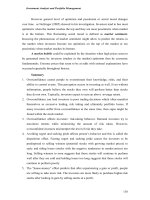
These differences in yields are referred to as yield spreads, and these yield spreads change
over time. As an example, if the yield on a portfolio of Aaa-rated bonds is 7.50 percent and the
yield on a portfolio of Baa-rated bonds is 9.00 percent, we would say that the yield spread is
1.50 percent. This 1.50 percent is referred to as a credit risk premium because the Baa-rated bond
is considered to have higher credit risk—that is, greater probability of default. This Baa–Aaa yield
spread is not constant over time. For an example of changes in a yield spread, note the substan-
tial changes in the yield spreads on Aaa-rated bonds and Baa-rated bonds shown in Exhibit 1.9.

Although the underlying risk factors for the portfolio of bonds in the Aaa-rated bond index and
the Baa-rated bond index would probably not change dramatically over time, it is clear from the
time-series plot in Exhibit 1.9 that the difference in yields (i.e., the yield spread) has experienced
changes of more than 100 basis points (1 percent) in a short period of time (for example, see the
yield spread increase in 1974 to 1975 and the dramatic yield spread decline in 1983 to 1984). Such
a significant change in the yield spread during a period where there is no major change in the risk
characteristics of Baa bonds relative to Aaa bonds would imply a change in the market RP. Specif-
ically, although the risk levels of the bonds remain relatively constant, investors have changed the
yield spreads they demand to accept this relatively constant difference in risk.
This change in the RP implies a change in the slope of the SML. Such a change is shown in
Exhibit 1.10. The exhibit assumes an increase in the market risk premium, which means an
increase in the slope of the market line. Such a change in the slope of the SML (the risk pre-
mium) will affect the required rate of return for all risky assets. Irrespective of where an invest-
ment is on the original SML, its required rate of return will increase, although its individual risk
characteristics remain unchanged.
The graph in Exhibit 1.11 shows what happens to the SML when there are changes in one of
the following factors: (1) expected real growth in the economy, (2) capital market conditions, or
(3) the expected rate of inflation. For example, an increase in expected real growth, temporary
tightness in the capital market, or an increase in the expected rate of inflation will cause the SML
to experience a parallel shift upward. The parallel shift occurs because changes in expected real
growth or in capital market conditions or a change in the expected rate of inflation affect all
investments, no matter what their levels of risk are.
Changes in Capital
Market Conditions
or Expected
Inflation
R
ELATIONSHIP BETWEEN RISK AND RETURN 25
26 CHAPTER 1 THE INVESTMENT SETTING
1966 19941968 1970 1972 1974 1976 1978 1980 1982 1984 1986 1988 1990 1992

3.0
2.5
2.0
1.5
1.0
0.5
0.0
Yield Spread
1996 1998
Year
2000
EXHIBIT 1.9
PLOT OF MOODY’S CORPORATE BOND YIELD SPREADS (BAA–AAA): MONTHLY 1966–2000
Risk
Original SML
Expected Return
New SML
R
m
R
m
′
NRFR
•
•
•
EXHIBIT 1.10
CHANGE IN MARKET RISK PREMIUM