advances in Investment Analysis and Portfolio Management phần 4 pptx

Investment Analysis and Portfolio Management
50

a) Calculate the main statistic measures to explain the relationship between stock
A and the market portfolio:
• The sample covariance between rate of return for the stock A and the
market;
• The sample Beta factor of stock A;
• The sample correlation coefficient between the rates of return of the
stock A and the market;
• The sample coefficient of determination associated with the stock A and
the market.
b) Draw in the characteristic line of the stock A and give the interpretation - what
does it show for the investor?
c) Calculate the sample residual variance associated with stock‘s A characteristic
line and explain how the investor would interpret the number of this statistic.
d) Do you recommend this stock for the investor with the lower tolerance of risk?
References and further readings
1. Fabozzi, Frank J. (1999). Investment Management. 2nd. ed. Prentice Hall Inc.
2. Francis, Jack, C. Roger Ibbotson (2002). Investments: A Global Perspective.
Prentice Hall Inc.
3. Haugen, (Robert A. 2001). Modern Investment Theory. 5
th
ed. Prentice Hall.
4. Levy, Haim, Thierry Post (2005). Investments. FT / Prentice Hall.
5. Rosenberg, Jerry M. (1993).Dictionary of Investing. John Wiley &Sons Inc.
6. Sharpe, William F., Gordon J.Alexander, Jeffery V.Bailey. (1999). Investments.
International edition. Prentice –Hall International.
7. Strong, Robert A. (1993). Portfolio Construction, Management and Protection.

Investment Analysis and Portfolio Management
51

3. Theory for investment portfolio formation
Mini-contents
3.1. Portfolio theory.
3.1.1. Markowitz portfolio theory.
3.1.2. The Risk and Expected Return of a Portfolio.
3.2. Capital Asset Pricing Model (CAPM).
3.3. Arbitrage Pricing Theory (APT).
3.4. Market efficiency theory.
Summary
Key terms
Questions and problems
References and further readings


3.1. Portfolio theory

3.1.1. Markowitz portfolio theory
The author of the modern portfolio theory is Harry Markowitz who introduced
the analysis of the portfolios of investments in his article “Portfolio Selection”
published in the Journal of Finance in 1952. The new approach presented in this article
included portfolio formation by considering the expected rate of return and risk of
individual stocks and, crucially, their interrelationship as measured by correlation.
Prior to this investors would examine investments individually, build up portfolios of
attractive stocks, and not consider how they related to each other. Markowitz showed
how it might be possible to better of these simplistic portfolios by taking into account
the correlation between the returns on these stocks.
The diversification plays a very important role in the modern portfolio theory.
Markowitz approach is viewed as a single period approach: at the beginning of the
period the investor must make a decision in what particular securities to invest and
hold these securities until the end of the period. Because a portfolio is a collection of
securities, this decision is equivalent to selecting an optimal portfolio from a set of
possible portfolios. Essentiality of the Markowitz portfolio theory is the problem of
optimal portfolio selection.
The method that should be used in selecting the most desirable portfolio involves
the use of indifference curves. Indifference curves represent an investor’s preferences
for risk and return. These curves should be drawn, putting the investment return on the
vertical axis and the risk on the horizontal axis. Following Markowitz approach, the
Investment Analysis and Portfolio Management
52

measure for investment return is expected rate of return and a measure of risk is
standard deviation (these statistic measures we discussed in previous chapter, section
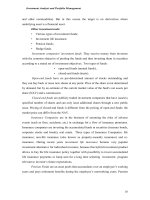
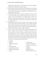
2.1). The exemplified map of indifference curves for the individual risk-averse
investor is presented in Fig.3.1. Each indifference curve here (I
1,
I

2
, I3

) represents the
most desirable investment or investment portfolio for an individual investor. That
means, that any of investments (or portfolios) ploted on the indiference curves (A,B,C
or D) are equally desirable to the investor.

Features of indifference curves:
 All portfolios that lie on a given indifference curve are equally desirable to
the investor. An implication of this feature: indifference curves cannot
intersect.
 An investor has an infinitive number of indifference curves. Every investor
can represent several indifference curves (for different investment tools).
Every investor has a map of the indifference curves representing his or her
preferences for expected returns and risk (standard deviations) for each
potential portfolio.

Fig. 3.1. Map of Indiference Curves for a Risk-Averse Investor

Two important fundamental assumptions than examining indifference curves
and applying them to Markowitz portfolio theory:
1. The investors are assumed to prefer higher levels of return to lower levels
of return, because the higher levels of return allow the investor to spend
more on consumption at the end of the investment period. Thus, given two
portfolios with the same standard deviation, the investor will choose the
Risk (

D

B



C

r

B

r

C

r

A

r

D


I
1

I
2

I

3

σ

B

σ

D

σ

C

σ

A

σ

A

Expected
rate of
return (

)


r

)

Investment Analysis and Portfolio Management
53

portfolio with the higher expected return. This is called an assumption of
nonsatiation.
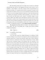
2. Investors are risk averse. It means that the investor when given the choise,
will choose the investment or investment portfolio with the smaller risk.
This is called assumption of risk aversion.
















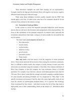
Fig. 3.2. Portfolio choise using the assumptions of nonsatiation and risk aversion

Fig. 3.2. gives an example how the investor chooses between 3 investments –

A,B and C. Following the assumption of nonsatiation, investor will choose A or B
which have the higher level of expected return than C. Following the assumption of
risk aversion investor will choose A, despite of the same level of expected returns for
investment A and B, because the risk (standard deviation) for investment A is lower
than for investment B. In this choise the investor follows so called „furthest
northwest“ rule.
In reality there are an infinitive number of portfolios available for the
investment. Is it means that the investor needs to evaluate all these portfolios on return
and risk basis? Markowitz portfolio theory answers this question using efficient set
theorem: an investor will choose his/ her optimal portfolio from the set of the
portfolios that (1) offer maximum expected return for varying level of risk, and (2)
offer minimum risk for varying levels of expected return.
Efficient set of portfolios involves the portfolios that the investor will find
optimal ones. These portfolios are lying on the “northwest boundary” of the feasible
set and is called an efficient frontier. The efficient frontier can be described by the
C

B

A

=

=

r

A

r

B

r

C

σ

A

σ

C

σ

B

Expected
rate of
return (

Risk (

σ


)

r

)

Investment Analysis and Portfolio Management
54

curve in the risk-return space with the highest expected rates of return for each level of
risk.
Feasible set is opportunity set, from which the efficient set of portfolio can
be identified. The feasibility set represents all portfolios that could be formed from the
number of securities and lie either or or within the boundary of the feasible set.
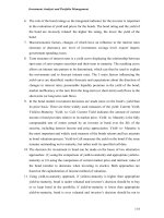
In Fig.3.3 feasible and efficient sets of portfolios are presented. Considering
the assumptions of nonsiation and risk aversion discussed earlier in this section, only
those portfolios lying between points A and B on the boundary of feasibility set
investor will find the optimal ones. All the other portfolios in the feasible set are are
inefficient portfolios. Furthermore, if a risk-free investment is introduced into the
universe of assets, the efficient frontier becomes the tagental line shown in Fig. 3.3 this
line is called the Capital Market Line (CML) and the portfolio at the point at which it
is tangential (point M) is called the Market Portolio.

Fig.3.3. Feasible Set and Efficient Set of Portfolios (Efficient Frontier)


3.1.2. The Expected Rate of Return and Risk of Portfolio

Following Markowitz efficient set portfolios approach an investor should
evaluate alternative portfolios inside feasibility set on the basis of their expected
returns and standard deviations using indifference curves. Thus, the methods for
calculating expected rate of return and standard deviation of the portfolio must be
discussed.
A

M

C

A

Feasible
set

B

C

D

Risk (

Expected
rate of
return





σ

P

)

Risk
free rate

Capital Market
Line

Efficient
Frontier

Investment Analysis and Portfolio Management
55

The expected rate of return of the portfolio can be calculated in some
alternative ways. The Markowitz focus was on the end-of-period wealth (terminal
value) and using these expected end-of-period values for each security in the portfolio
the expected end-of-period return for the whole portfolio can be calculated. But the
portfolio really is the set of the securities thus the expected rate of return of a portfolio
should depend on the expected rates of return of each security included in the portfolio
(as was presented in Chapter 2, formula 2.4). This alternative method for calculating
the expected rate of return on the portfolio (E
(r)p
) is the weighted average of the
expected returns on its component securities:
n
E
(r)p
= Σ w
i
* E
i
(r) = E
1
(r)

+ w
2
* E
2
(r)

+…+ w
n
* E
n
(r),

(3.1)


i=1

here wi - the proportion of the portfolio’s initial value invested in security i;
E
i
(r) - the expected rate of return of security I;
n - the number of securities in the portfolio.
Because a portfolio‘s expected return is a weighted average of the expected
returns of its securities, the contribution of each security to the portfolio‘s expected
rate of return depends on its expected return and its proportional share from the initial
portfolio‘s market value (weight). Nothing else is relevant. The conclusion here could
be that the investor who simply wants the highest posible expected rate of return must
keep only one security in his portfolio which has a highest expected rate of return. But
why the majority of investors don‘t do so and keep several different securities in their
portfolios? Because they try to diversify their portfolios aiming to reduce the
investment portfolio risk.
Risk of the portfolio. As we know from chapter 2, the most often used
measure for the risk of investment is standard deviation, which shows the volatility of
the securities actual return from their expected return. If a portfolio‘s expected rate of
return is a weighted average of the expected rates of return of its securities, the

calculation of standard deviation for the portfolio can‘t simply use the same approach.
The reason is that the relationship between the securities in the same portfolio must be
taken into account. As it was discussed in section 2.2, the relationship between the
assets can be estimated using the covariance and coefficient of correlation. As
covariance can range from “–” to “+” infinity, it is more useful for identification of
the direction of relationship (positive or negative), coefficients of correlation always
Investment Analysis and Portfolio Management
56

lies between -1 and +1 and is the convenient measure of intensity and direction of the
relationship between the assets.
Risk of the portfolio, which consists of 2 securities (A ir B):

δ
δδ
δ
p
=
(
w²
A
×
××
× δ
δδ
δ²
A
+ w²
B
×

××
×δ
δδ
δ²
B
+ 2 w
A
×
××
× w
B
×
××
× k
AB
×
××
× δ
δδ
δ
A
×
××
×δ
δδ
δ
B
)
1/2
, (3.2)

here: w
A
ir w
B
- the proportion of the portfolio’s initial value invested in security A
and B ( wA + wB = 1);
δ
A
ir δ
B
- standard deviation of security A and B;
k
AB
- coefficient of coreliation between the returns of security A and B.
Standard deviation of the portfolio consisting n securities:

n n

δ
δδ
δ =

(
∑
∑∑
∑ ∑
∑∑
∑ w
i

w
j
k
ij
δ
δδ
δ
i
δ
δδ
δ
j
)
1/2
, (3.3)

i=1 j=1

here: w
i
ir w
j
- the proportion of the portfolio’s initial value invested in security i
and j ( wi + wj = 1);
δ
i
ir δ
j
- standard deviation of security i and j;
k

ij
- coefficient of coreliation between the returns of security i and j.

3.2. Capital Asset Pricing Model (CAPM)

CAPM was developed by W. F. Sharpe. CAPM simplified Markowitz‘s Modern
Portfolio theory, made it more practical. Markowitz showed that for a given level of
expected return and for a given feasible set of securities, finding the optimal portfolio
with the lowest total risk, measured as variance or standard deviation of portfolio
returns, requires knowledge of the covariance or correlation between all possible
security combinations (see formula 3.3). When forming the diversified portfolios
consisting large number of securities investors found the calculation of the portfolio
risk using standard deviation technically complicated.
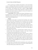
Measuring Risk in CAPM is based on the identification of two key
components of total risk (as measured by variance or standard deviation of return):
 Systematic risk
 Unsystematic risk
Systematic risk is that associated with the market (purchasing power risk,
interest rate risk, liquidity risk, etc.)
Investment Analysis and Portfolio Management
57

Unsystematic risk is unique to an individual asset (business risk, financial risk,
other risks, related to investment into particular asset).
Unsystematic risk can be diversified away by holding many different assets in
the portfolio, however systematic risk can’t be diversified (see Fig 3.4). In CAPM
investors are compensated for taking only systematic risk. Though, CAPM only links
investments via the market as a whole.

Portfolio Risk

0 1 2 3 4 5 6 7 8 9 10

Number of securities in portfolio

Fig.3.4. Portfolio risk and the level of diversification

The essence of the CAPM: the more systematic risk the investor carry, the
greater is his / her expected return.
The CAPM being theoretical model is based on some important assumptions:
• All investors look only one-period expectations about the future;
• Investors are price takers and they cant influence the market individually;
• There is risk free rate at which an investors may either lend (invest) or
borrow money.
• Investors are risk-averse,
• Taxes and transaction costs are irrelevant.
• Information is freely and instantly available to all investors.
Following these assumptions, the CAPM predicts what an expected rate of
return for the investor should be, given other statistics about the expected rate of
return in the market and market risk (systematic risk):

Systematic risk
Unsyste
matic risk

Total risk

Investment Analysis and Portfolio Management
58

E(r
j
)

= R
f
+ β
ββ
β
(j)
* ( E(r
M)
- R
f
), (
3.4)

here: E(r
j
)

- expected return on stock j;
R
f
- risk free rate of return;
E(r
M)
- expected rate of return on the market
β
(j)

- coefficient Beta, measuring undiversified risk of security j.
Several of the assumptions of CAPM seem unrealistic. Investors really are
concerned about taxes and are paying the commisions to the broker when bying or
selling their securities. And the investors usually do look ahead more than one period.
Large institutional investors managing their portfolios sometimes can influence market
by bying or selling big ammounts of the securities. All things considered, the
assumptions of the CAPM constitute only a modest gap between the thory and reality.
But the empirical studies and especially wide use of the CAPM by practitioners show
that it is useful instrument for investment analysis and decision making in reality.
As can be seen in Fig.3.5, Equation in formula 3.4 represents the straight line
having an intercept of R
f
and slope of

β
(j
) * ( E(r
M)
- R
f
). This relationship between
the expected return and Beta is known as Security Market Line (SML). Each security
can be described by its specific security market line, they differ because their Betas are
different and reflect different levels of market risk for these securities.

Fig.3.5. Security Market Line (SML)

Coefficient Beta (β
ββ
β). Each security has it’s individual systematic -
undiversified risk, measured using coefficient Beta. Coefficient Beta (β) indicates how
the price of security/ return on security depends upon the market forces (note: CAPM
uses the statistic measures which we examined in section 2.3, including Beta factor).
Thus, coefficient Beta for any security can be calculated using formula 2.14:
K

M
L

1.0

E(r
)

R

f

β

SML
SML
1

SML
r

L

r

K

r

M

Investment Analysis and Portfolio Management
59

Cov (r
J
,r
M
)


β
J

=
δ²(r
M

Table 3.1
Interpretation of coefficient Beta (β
ββ
β)

Beta Direction of changes
in security’s return
in comparison to the
changes in market’s
return
Interpretation of β
ββ
β meaning

2,0
The same as market Risk of security is twice higher than market risk
1,0
The same as market Security’s risk is equal to market risk
0,5 The same as market Security’s risk twice lower than market risk
0 There is no
relationship
Security’s risk are not influenced by market risk
Minus
0,5
The opposite from the
market

Security’s risk twice lower than market risk, but in
opposite direction
Minus
1,0
The opposite from the
market
Security’s risk is equal to market risk but in
opposite direction
Minus
2,0
The opposite from the
market
Risk of security is twice higher than market risk,
but in opposite direction

One very important feature of Beta to the investor is that the Beta of portfolio is
simply a weighted average of the Betas of its component securities, where the
proportions invested in the securities are the respective weights. Thus, Portfolio Beta
can be calculated using formula:

n

β
p
= w
1
β
1
+ w
2

β
2
+ + w
n
β
n

= ∑ w
i
* β
i ,
(3.5)

i=1

here w
i
- the proportion of the portfolio’s initial value invested in security i;
β
i
- coefficient Beta for security i.
Earlier it was shown that the expected return on the portfolio is a weighted
average of the expected returns of its components securities, where the proportions
invested in the securities are the weights. This meas that because every security plots o
the SML, so will every portfolio. That means, that not only every security, but also
every portfolio must plot on an upward sloping straight line in a diagram (3.5) with the
expected return on the vertical axis and Beta on the horizontal axis.

3.3.Arbitrage Pricing Theory (APT)

APT was propsed ed by Stephen S.Rose and presented in his article „The
arbitrage theory of Capital Asset Pricing“, published in Journal of Economic Theory in
Investment Analysis and Portfolio Management
60

1976. Still there is a potential for it and it may sometimes displace the CAPM. In the
CAPM returns on individual assets are related to returns on the market as a whole. The
key point behind APT is the rational statement that the market return is determined by
a number of different factors. These factors can be fundamental factors or statistical. If
these factors are essential, there to be no arbitrage opportunities there must be
restrictions on the investment process. Here arbitrage we understand as the earning of
riskless profit by taking advantage of differential pricing for the same assets or
security. Arbitrage is is widely applied investment tactic.
APT states, that the expected rate of return of security J is the linear function
from the complex economic factors common to all securities and can be estimated
using formula:
E(r
J
)

= E(ŕ
J)
+ β
1J
I
1J
+ β
2J
I
2J

+ + β
nJ
I
nJ
+ ε
J
, (3.6)

here: E(r
J
)

- expected return on stock J;
E(ŕ
J)
- expected rate of return for security J, if the influence of all factors is
0;
I
iJ
- the change in the rate of return for security J, influenced by economic
factor i (i = 1, , n);
β
iJ
- coefficient Beta, showing sensitivity of security’s J rate of return
upon the factor i (this influence could be both positive or negative);
ε
J
- error of rounding for the security J (expected value – 0).
It is important to note that the arbitrage in the APT is only approximate,
relating diversified portfolios, on assumption that the asset unsystematic (specific)

risks are negligable compared with the factor risks.
There could presumably be an infinitive number of factors, although the
empirical research done by S.Ross together with R. Roll (1984) identified four factors
– economic variables, to which assets having even the same CAPM Beta, are
differently sensitive:
• inflation;
• industrial production;
• risk premiums;
• slope of the term structure in interst rates.
Investment Analysis and Portfolio Management
61

In practice an investor can choose the macroeconomic factors which seems
important and related with the expected returns of the particular asset. The examples
of possible macroeconomic factors which could be included in using APT model :
• GDP growth;
• an interest rate;
• an exchange rate;
• a defaul spread on corporate bonds, etc.
Including more factors in APT model seems logical. The institutional investors
and analysts closely watch macroeconomic statistics such as the money supply,
inflation, interest rates, unemployment, changes in GDP, political events and many
others. Reason for this might be their belief that new information about the changes in
these macroeconomic indicators will influence future asset price movements. But it is
important to point out that not all investors or analysts are concerned with the same set
of economic information and they differently assess the importance of various
macroeconomic factors to the assets they have invested already or are going to invest.
At the same time the large number of the factors in the APT model would be
impractical, because the models seldom are 100 percent accurate and the asset prices
are function of both macroeconomic factors and noise. The noise is coming from

minor factors, with a little influence to the result – expected rate of return.
The APT does not require identification of the market portfolio, but it does
reguire the specification of the relevant macroeconomic factors. Much of the current
empirical APT research are focused on identification of these factors and the
determination of the factors’ Betas. And this problem is still unsolved. Although more
than two decades have passed since S. Ross introduced APT model, it has yet to reach
the practical application stage.
The CAPM and APT are not really essentially different, because they are
developed for determing an expected rate of return based on one factor (market
portfolio – CAPM) or a number of macroeconomic factors (APT). But both models
predict how the return on asset will result from factor sensitivities and this is of great
importance to the investor.



Investment Analysis and Portfolio Management
62

3.4. Market efficiency theory
The concept of market efficiency was proposed by Eugene Fama in 1965, when
his article “Random Walks in Stock Prices” was published in Financial Analyst
Journal.
Market efficiency means that the price which investor is paying for financial
asset (stock, bond, other security) fully reflects fair or true information about the
intrinsic value of this specific asset or fairly describe the value of the company – the
issuer of this security. The key term in the concept of the market efficiency is the
information available for investors trading in the market. It is stated that the market
price of stock reflects:
1. All known information, including:
 Past information, e.g., last year’s or last quarter’s, month’s

earnings;
 Current information as well as events, that have been announced but
are still forthcoming, e.g. shareholders’ meeting.
2. Information that can reasonably be inferred, for example, if many investors
believe that ECB will increase interest rate in the nearest future or the government
deficit increases, prices will reflect this belief before the actual event occurs.
Capital market is efficient, if the prices of securities which are traded in the
market, react to the changes of situation immediately, fully and credibly reflect all the
important information about the security’s future income and risk related with
generating this income.
What is the important information for the investor? From economic point of
view the important information is defined as such information which has direct
influence to the investor’s decisions seeking for his defined financial goals. Example,
the essential events in the joint stock company, published in the newspaper, etc.
Market efficiency requires thet the adjustment to new information occurs very
quikly as the information becomes known. Obvious, that Internet has made the markets
more efficient in the sense of how widely and quickly information is disseminated.
There are 3 forms of market efficiency under efficient market hypothesis:
• Weak form of efficiency;
• Semi- strong form of efficiency;
• Strong form of the efficiency.
Investment Analysis and Portfolio Management
63

Under the weak form of efficiency stock prices are assumed to reflect any
information that may be contained in the past history of the stock prices. So, if the
market is characterized by weak form of efficiency, no one investor or any group of
investors should be able to earn over the defined period of time abnormal rates of
return by using information about historical prices available for them and by using
technical analysis. Prices will respond to news, but if this news is random then price

changes will also be random.
Under the semi-strong form of efficiency all publicly available information is
presumed to be reflected in stocks’ prices. This information includes information in the
stock price series as well as information in the firm’s financial reports, the reports of
competing firms, announced information relating to the state of the economy and any
other publicly available information, relevant to the valuation of the firm. Note that
the market with a semi strong form of efficiency encompasies the weak form of the
hypothesis because the historical market data are part of the larger set of all publicly
available information. If the market is characterized by semi-strong form of efficiency,
no one investor or any group of investors should be able to earn over the defined
period of time abnormal rates of return by using information about historical prices
and publicly available fundamental information(such as financial statemants) and
fundamental analysis.
The strong form of efficiency which asserts that stock prices fully reflect all
information, including private or inside information, as well as that which is publicly
available. This form takes the notion of market efficiency to the ultimate extreme.
Under this form of market efficiency securities’ prices quickly adjust to reflect both
the inside and public information. If the market is characterized by strong form of
efficiency, no one investor or any group of investors should be able to earn over the
defined period of time abnormal rates of return by using all information available for
them.
The validity of the market efficiency hypothesis whichever form is of great
importance to the investors because it determines whether anyone can outperform the
market, or whether the successful investing is all about luck. Efficient market
hypothesis does not require to behave rationally, only that in response to information
there will be a sufficiently large random reaction that an excess profit cannot be made.
Investment Analysis and Portfolio Management
64

The concept of the market efficiency now is criticezed by some market analysts

and participants by stating that no one market can be fully efficient as some irrational
behavior of investors in the market occurs which is more based on their emotions and
other psychological factors than on the information available (the psychological
aspects of investment decision making will be disscussed further, in chapter 6). But, at
the same time, it can be shown that the efficient market can exist, if in the real markets
following events occur:
 A large number of rational, profit maximizing investors exist who are
actively and continuously analyzing valuing and trading securities;
 Information is widely available to market participants at the same time
and without or very small cost;
 Information is generated in a random walk manner and can be treated as
independent;
 Investors react to the new information quickly and fully, though causing
market prices to adjust accordingly.
Summary

1. Essentiality of the Markowitz portfolio theory is the problem of optimal portfolio
selection. The Markowitz approach included portfolio formation by considering
the expected rate of return and risk of individual stocks measured as standard
deviation, and their interrelationship as measured by correlation. The
diversification plays a key role in the modern portfolio theory.
2. Indifference curves represent an investor’s preferences for risk and return. These
curves should be drawn, putting the investment return on the vertical axis and the
risk on the horizontal axis.
3. Two important fundamental assumptions than applying indifference curves to
Markowitz portfolio theory. An assumption of nonsatiation assumes that the
investors prefer higher levels of return to lower levels of return, because the
higher levels of return allow the investor to spend more on consumption at the
end of the investment period. An assumption of risk aversion assumes that the
investor when given the choise, will choose the investment or investment

portfolio with the smaller risk, i.e. the investors are risk averse.

Investment Analysis and Portfolio Management
65

4. Efficient set theorem states that an investor will choose his/ her optimal portfolio
from the set of the portfolios that (1) offer maximum expected return for varying
level of risk, and (2) offer minimum risk for varying levels of expected return.
5. Efficient set of portfolios involves the portfolios that the investor will find
optimal ones. These portfolios are lying on the “northwest boundary” of the
feasible set and is called an efficient frontier. The efficient frontier can be
described by the curve in the risk-return space with the highest expected rates of
return for each level of risk. Feasible set is opportunity set, from which the
efficient set of portfolio can be identified. The feasibility set represents all
portfolios that could be formed from the number of securities and lie either or or
within the boundary of the feasible set.
6. Capital Market Line (CML) shows the trade off-between expected rate of return
and risk for the efficient portfolios under determined risk free return.
7. The expected rate of return on the portfolio is the weighted average of the
expected returns on its component securities.
8. The calculation of standard deviation for the portfolio can‘t simply use the
weighted average approach. The reason is that the relationship between the
securities in the same portfolio measured by coefficient of correlation must be
taken into account. When forming the diversified portfolios consisting large
number of securities investors found the calculation of the portfolio risk using
standard deviation technically complicated.
9. Measuring Risk in Capital asset Pricing Model (CAPM) is based on the
identification of two key components of total risk: systematic risk and
unsystematic risk. Systematic risk is that associated with the market.
Unsystematic risk is unique to an individual asset and can be diversified away by

holding many different assets in the portfolio. In CAPM investors are
compensated for taking only systematic risk.
10. The essence of the CAPM: CAPM predicts what an expected rate of return for
the investor should be, given other statistics about the expected rate of return in
the market, risk free rate of return and market risk (systematic risk).
11. Each security has it’s individual systematic - undiversified risk, measured using
coefficient Beta. Coefficient Beta (β) indicates how the price of security/ return
on security depends upon the market forces. The Beta of the portfolio is simply a