Tin học ứng dụng trong công nghệ hóa học Parallelprocessing 6 speedup

Speedup

Thoai Nam


Outline





Speedup & Efficiency
Amdahl’s Law
Gustafson’s Law
Sun & Ni’s Law

Khoa Khoa học và Kỹ thuật Máy tính - ĐHBK TP.HCM


Speedup & Efficiency




Speedup:
S = Time(the most efficient sequential
algorithm) / Time(parallel algorithm)
Efficiency:
E=S/N
with N is the number of processors

Khoa Khoa học và Kỹ thuật Máy tính - ĐHBK TP.HCM


Amdahl’s Law – Fixed Problem
Size (1)


The main objective is to produce the results as
soon as possible
– (ex) video compression, computer graphics, VLSI routing,
etc



Implications
– Upper-bound is
– Make Sequential bottleneck as small as possible
– Optimize the common case



Modified Amdahl’s law for fixed problem size
including the overhead
Khoa Khoa học và Kỹ thuật Máy tính - ĐHBK TP.HCM


Amdahl’s Law – Fixed Problem
Size (2)
Sequential

Sequential

Parallel

Ts

Tp
T(1)

Parallel

Sequential

P0 P1 P2 P3 P 4 P5 P6 P7 P8 P9

T(N)

Ts=T(1)  Tp= (1-)T(1)
T(N) = T(1)+ (1-)T(1)/N
Khoa Khoa học và Kỹ thuật Máy tính - ĐHBK TP.HCM

Number of
processors


Amdahl’s Law – Fixed Problem
Size (3)
Time(1)
Speedup 
Time( N )

T (1)
1
1
Speedup 

 as N  
(1   )T (1)
(1   )

T (1) 

N
N

Khoa Khoa học và Kỹ thuật Máy tính - ĐHBK TP.HCM


Enhanced Amdahl’s Law
The overhead includes parallelism
and interaction overheads
T (1)
1
Speedup 

as N  
(1   )T (1)
Toverhead
T (1) 
 Toverhead


N
T (1)

Khoa Khoa học và Kỹ thuật Máy tính - ĐHBK TP.HCM


Gustafson’s Law – Fixed Time (1)


User wants more accurate results within a time limit
– Execution time is fixed as system scales
– (ex) FEM (Finite element method) for structural analysis, FDM
(Finite difference method) for fluid dynamics



Properties of a work metric
–
–
–
–
–



Easy to measure
Architecture independent
Easy to model with an analytical expression
No additional experiment to measure the work
The measure of work should scale linearly with sequential time

complexity of the algorithm

Time constrained seems to be most generally viable
model!
Khoa Khoa học và Kỹ thuật Máy tính - ĐHBK TP.HCM


Gustafson’s Law – Fixed Time (2)
P9
.
.
.

Parallel

Sequential

P0

Ws

W0

 = Ws / W(N)
W(N) = W(N) + (1-)W(N)
 W(1) = W(N) + (1-)W(N)N

W(N)

Sequential

Sequential

P0 P 1 P2 P3 P4 P5 P6 P7 P8 P9

Khoa Khoa học và Kỹ thuật Máy tính - ĐHBK TP.HCM


Gustafson’s Law – Fixed Time
without overhead
Time = Work . k
W(N) = W
T (1)
W (1).k W  (1    NW
Speedup 


   (1   ) N
T ( N ) W ( N ).k
W

Khoa Khoa học và Kỹ thuật Máy tính - ĐHBK TP.HCM


Gustafson’s Law – Fixed Time
with overhead
W(N) = W + W0
Speedup 

T (1)

W (1).k W  (1    NW   (1    N



W0
T ( N ) W ( N ).k
W  W0
1
W

Khoa Khoa học và Kỹ thuật Máy tính - ĐHBK TP.HCM


Sun and Ni’s Law –
Fixed Memory (1)




Scale the largest possible solution limited by
the memory space. Or, fix memory usage per
processor
Speedup,
– Time(1)/Time(N) for scaled up problem is not
appropriate.
– For simple profile, and G(N) is the increase of
parallel workload as the memory capacity
increases N times.

Khoa Khoa học và Kỹ thuật Máy tính - ĐHBK TP.HCM

Sun and Ni’s Law –
Fixed Memory (2)






W=W+(1- )W
Let M be the memory capacity of a single
node
N nodes:
– the increased memory N*M
– The scaled work: W=W+(1- )G(N)W

Speedup MC 

  (1   )G ( N )
G( N )
  (1   )
N

Khoa Khoa học và Kỹ thuật Máy tính - ĐHBK TP.HCM


Sun and Ni’s Law –
Fixed Memory (3)


Definition:
A function g is homomorphism if there exists a function g
such that for any real number c and variable x,
g (cx)  g (c) g ( x) .



Theorem:
If W = g (M ) for some homomorphism function g ,
g (cx)  g (c) g ( x) , then, with all data being shared by all
available processors, the simplified memory-bounced
speedup is
W1  g ( N )WN
  (1   )G ( N )
*
SN 

g (N )
G( N )
W1 
WN   (1   )
N
N
Khoa Khoa học và Kỹ thuật Máy tính - ĐHBK TP.HCM


Sun and Ni’s Law –
Fixed Memory (4)
Proof:

Let the memory requirement of Wn be M, Wn = g (M ) .
M is the memory requirement when 1 node is available.
With N nodes available, the memory capacity will increase
to N*M.
Using all of the available memory, for the scaled parallel
*
*
W
W
portion N : N  g ( NM )  g ( N ) g (M )  g ( N )WN
.

*
*
W

W
W1  g ( N )WN
*
1
N
SN 

*
WN W  g ( N ) W
*
W1 
1
N
N

N

Khoa Khoa học và Kỹ thuật Máy tính - ĐHBK TP.HCM


Speedup
W1  G ( N )WN
S 
G( N )
W1 
WN
N
*
N

– When the problem size is independent of the system, the
problem size is fixed, G(N)=1  Amdahl’s Law.
– When memory is increased N times, the workload also
increases N times, G(N)=N  Gustafson’s Law
– For most of the scientific and engineering applications, the
computation requirement increases faster than the
memory requirement, G(N)>N.

Khoa Khoa học và Kỹ thuật Máy tính - ĐHBK TP.HCM


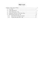
Examples
10

6

S(Linear)
S(Normal)

4
2

10

8

6

4

2

0

0

Speedup

8

Processors
Khoa Khoa học và Kỹ thuật Máy tính - ĐHBK TP.HCM


Scalability







Parallelizing a code does not always result in a speedup;
sometimes it actually slows the code down! This can be due
to a poor choice of algorithm or to poor coding
The best possible speedup is linear, i.e. it is proportional to
the number of processors: T(N) = T(1)/N where N = number
of processors, T(1) = time for serial run.
A code that continues to speed up reasonably close to
linearly as the number of processors increases is said to be
scalable. Many codes scale up to some number of
processors but adding more processors then brings no
improvement. Very few, if any, codes are indefinitely
scalable.
Khoa Khoa học và Kỹ thuật Máy tính - ĐHBK TP.HCM


Factors That Limit Speedup


Software overhead
Even with a completely equivalent algorithm, software overhead arises in
the concurrent implementation. (e.g. there may be additional index
calculations necessitated by the manner in which data are "split up"
among processors.)
i.e. there is generally more lines of code to be executed in the parallel

program than the sequential program.




Load balancing
Communication overhead

Khoa Khoa học và Kỹ thuật Máy tính - ĐHBK TP.HCM