Ch4 2 v1 TRUYỀN SỐ LIỆU VÀ MẠNG
Bạn đang xem bản rút gọn của tài liệu. Xem và tải ngay bản đầy đủ của tài liệu tại đây (808.64 KB, 43 trang )
Chapter 4
Digital Transmission
4.1
Copyright © The McGraw-Hill Companies, Inc. Permission required for reproduction or display.
4-2 ANALOG-TO-DIGITAL CONVERSION
A digital signal is superior to an analog signal because
it is more robust to noise and can easily be recovered,
corrected and amplified. For this reason, the tendency
today is to change an analog signal to digital data. In
this section we describe two techniques, pulse code
modulation and delta modulation.
Topics discussed in this section:
Pulse Code Modulation (PCM)
Delta Modulation (DM)
4.2
PCM
PCM consists of three steps to
digitize an analog signal:
1.
2.
3.
4.3
Sampling
Quantization
Binary encoding
Before we sample, we have to filter
the signal to limit the maximum
frequency of the signal as it affects
the sampling rate.
Filtering should ensure that we do
not distort the signal, ie remove
high frequency components that affect
the signal shape.
Figure 4.21 Components of PCM encoder
4.4
Sampling
Analog signal is sampled every TS secs.
Ts is referred to as the sampling
interval.
fs = 1/Ts is called the sampling rate or
sampling frequency.
There are 3 sampling methods:
4.5
Ideal - an impulse at each sampling instant
Natural - a pulse of short width with
varying amplitude
Flattop - sample and hold, like natural but
with single amplitude value
The process is referred to as pulse
amplitude modulation PAM and the
outcome is a signal with analog (non
integer) values
Figure 4.22 Three different sampling methods for PCM
4.6
Note
According to the Nyquist theorem, the
sampling rate must be
at least 2 times the highest frequency
contained in the signal.
4.7
Figure 4.23 Nyquist sampling rate for low-pass and bandpass signals
4.8
Example 4.6
For an intuitive example of the Nyquist theorem, let us
sample a simple sine wave at three sampling rates: fs = 4f (2
times the Nyquist rate), fs = 2f (Nyquist rate), and
fs = f (one-half the Nyquist rate). Figure 4.24 shows the
sampling and the subsequent recovery of the signal.
It can be seen that sampling at the Nyquist rate can create
a good approximation of the original sine wave (part a).
Oversampling in part b can also create the same
approximation, but it is redundant and unnecessary.
Sampling below the Nyquist rate (part c) does not produce
a signal that looks like the original sine wave.
4.9
Figure 4.24 Recovery of a sampled sine wave for different sampling rates
4.10
Example 4.7
Consider the revolution of a hand of a clock. The second
hand of a clock has a period of 60 s. According to the
Nyquist theorem, we need to sample the hand every 30 s
(Ts = T or fs = 2f ). In Figure 4.25a, the sample points, in
order, are 12, 6, 12, 6, 12, and 6. The receiver of the
samples cannot tell if the clock is moving forward or
backward. In part b, we sample at double the Nyquist rate
(every 15 s). The sample points are 12, 3, 6, 9, and 12.
The clock is moving forward. In part c, we sample below
the Nyquist rate (Ts = T or fs = f ). The sample points are
12, 9, 6, 3, and 12. Although the clock is moving forward,
the receiver thinks that the clock is moving backward.
4.11
Figure 4.25 Sampling of a clock with only one hand
4.12
Example 4.8
An example related to Example 4.7 is the seemingly
backward rotation of the wheels of a forward-moving car
in a movie. This can be explained by under-sampling. A
movie is filmed at 24 frames per second. If a wheel is
rotating more than 12 times per second, the undersampling creates the impression of a backward rotation.
4.13
Example 4.9
Telephone companies digitize voice by assuming a
maximum frequency of 4000 Hz. The sampling rate
therefore is 8000 samples per second.
4.14
Example 4.10
A complex low-pass signal has a bandwidth of 200 kHz.
What is the minimum sampling rate for this signal?
Solution
The bandwidth of a low-pass signal is between 0 and f,
where f is the maximum frequency in the signal.
Therefore, we can sample this signal at 2 times the
highest frequency (200 kHz). The sampling rate is
therefore 400,000 samples per second.
4.15
Example 4.11
A complex bandpass signal has a bandwidth of 200 kHz.
What is the minimum sampling rate for this signal?
Solution
We cannot find the minimum sampling rate in this case
because we do not know where the bandwidth starts or
ends. We do not know the maximum frequency in the
signal.
4.16
Quantization
4.17
Sampling results in a series of pulses
of varying amplitude values ranging
between two limits: a min and a max.
The amplitude values are infinite
between the two limits.
We need to map the infinite amplitude
values onto a finite set of known
values.
This is achieved by dividing the
distance between min and max into L
zones, each of height
= (max - min)/L
Quantization Levels
4.18
The midpoint of each zone is
assigned a value from 0 to L1 (resulting in L values)
Each sample falling in a zone
is then approximated to the
value of the midpoint.
Quantization Zones
4.19
Assume we have a voltage signal with
amplitutes Vmin=-20V and Vmax=+20V.
We want to use L=8 quantization
levels.
Zone width = (20 - -20)/8 = 5
The 8 zones are: -20 to -15, -15 to
-10, -10 to -5, -5 to 0, 0 to +5, +5
to +10, +10 to +15, +15 to +20
The midpoints are: -17.5, -12.5, 7.5, -2.5, 2.5, 7.5, 12.5, 17.5
Assigning Codes to
Each zone is then assigned a binary
Zones
code.
The number of bits required to encode
the zones, or the number of bits per
sample as it is commonly referred to, is
obtained as follows:
nb = log2 L
Given our example, nb = 3
The 8 zone (or level) codes are
therefore: 000, 001, 010, 011, 100, 101,
110, and 111
Assigning codes to zones:
4.20
000 will refer to zone -20 to -15
001 to zone -15 to -10, etc.