XỬ LÝ TÍN HIỆU SỐ Dsp chapter2 student 22062015
Bạn đang xem bản rút gọn của tài liệu. Xem và tải ngay bản đầy đủ của tài liệu tại đây (708.13 KB, 29 trang )
Chapter 2
Quantization
Nguyen Thanh Tuan, Click
M.Eng.
to edit Master subtitle style
Department of Telecommunications (113B3)
Ho Chi Minh City University of Technology
Email:
1. Quantization process
Fig: Analog to digital conversion
The quantized sample xQ(nT) is represented by B bit, which can take
2B possible values.
An A/D is characterized by a full-scale range R which is divided
into 2B quantization levels. Typical values of R in practice are
between 1-10 volts.
Digital Signal Processing
2
Quantization
1. Quantization process
Fig: Signal quantization
Quantizer resolution or quantization width (step) Q
R
R
A bipolar ADC xQ (nT )
2
2
R
2B
A unipolar ADC 0 xQ (nT ) R
Digital Signal Processing
3
Quantization
1. Quantization process
Quantization by rounding: replace each value x(nT) by the nearest
quantization level.
Quantization by truncation: replace each value x(nT) by its below
nearest quantization level.
Quantization error:
e(nT ) xQ (nT ) x(nT )
Consider rounding quantization:
Q
Q
e
2
2
Fig: Uniform probability density of quantization error
Digital Signal Processing
4
Quantization
1. Quantization process
The mean value of quantization error e
Q /2
Q /2
ep(e)de
Q /2
e
Q /2
Q /2
1
de 0
Q
Q /2
1
Q2
The mean-square error (power) e e p(e)de e de
Q
12
Q /2
Q /2
2
2
2
Root-mean-square (rms) error: erms e2
2
Q
12
R and Q are the ranges of the signal and quantization noise, then the
signal to noise ratio (SNR) or dynamic range of the quantizer is
defined as
R
SNR dB 20log10 20log10 (2 B ) B log10 (2) 6 B dB
Q
which is referred to as 6 dB bit rule.
Digital Signal Processing
5
Quantization
Example 1
In a digital audio application, the signal is sampled at a rate of 44
KHz and each sample quantized using an A/D converter having a
full-scale range of 10 volts. Determine the number of bits B if the
rms quantization error mush be kept below 50 microvolts. Then,
determine the actual rms error and the bit rate in bits per second.
Digital Signal Processing
6
Quantization
2. Digital to Analog Converters (DACs)
We begin with A/D converters, because they are used as the building
blocks of successive approximation ADCs.
Fig: B-bit D/A converter
Vector B input bits : b=[b1, b2,…,bB]. Note that bB is the least
significant bit (LSB) while b1 is the most significant bit (MSB).
For unipolar signal, xQ є [0, R); for bipolar xQ є [-R/2, R/2).
Digital Signal Processing
7
Quantization
2. DACs
Rf
Full scale R=VREF, B=4 bit
2Rf
4Rf
I
8Rf
MSB
i
xQ=Vout
16Rf
bB
b1
LSB
-VREF
Fig: DAC using binary weighted resistor
b1
b3
b2
b4
I
V
REF 2R 4R 8R 16R
f
f
f
f
b1 b2 b3 b4
xQ VOUT I R f VREF
2 4 8 16
xQ R24 b1 23 b2 22 b3 21 b4 20 Q b1 23 b2 22 b3 21 b4 20
Digital Signal Processing
8
Quantization
2. DACs
Unipolar natural binary xQ R(b1 21 b2 22 ... bB 2 B ) Qm
where m is the integer whose binary representation is b=[b1, b2,…,bB].
m b1 2B1 b2 2B2 ... bB 20
Bipolar offset binary: obtained by shifting the xQ of unipolar natural
binary converter by half-scale R/2:
R
R
xQ R(b1 2 b2 2 ... bB 2 ) Qm
2
2
1
2
B
Two’s complement code: obtained from the offset binary code by
complementing the most significant bit, i.e., replacing b1 by b1 1 b1 .
R
xQ R(b1 2 b2 2 ... bB 2 )
2
1
Digital Signal Processing
2
9
B
Quantization
Example 2
A 4-bit D/A converter has a full-scale R=10 volts. Find the quantized
analog values for the following cases ?
a) Natural binary with the input bits b=[1001] ?
b) Offset binary with the input bits b=[1011] ?
c) Two’s complement binary with the input bits b=[1101] ?
Digital Signal Processing
10
Quantization
3. A/D converters
A/D converters quantize an analog value x so that is is represented
by B bits b=[b1, b2,…,bB].
Fig: B-bit A/D converter
Digital Signal Processing
11
Quantization
3. A/D converters
One of the most popular converters is the successive approximation
A/D converter
Fig: Successive approximation A/D converter
After B tests, the successive approximation register (SAR) will hold
the correct bit vector b.
Digital Signal Processing
12
Quantization
3. A/D converters
Successive approximation algorithm
1 if x 0
where the unit-step function is defined by u ( x)
0 if x 0
This algorithm is applied for the natural and offset binary with
truncation quantization.
Digital Signal Processing
13
Quantization
Example 3
Consider a 4-bit ADC with the full-scale R=10 volts. Using the
successive approximation algorithm to find offset binary of
truncation quantization for the analog values x=3.5 volts and x=-1.5
volts.
Test b1b2b3b4
b1
b2
b3
b4
1000
1100
1110
1101
1101
Digital Signal Processing
xQ
C = u(x – xQ)
0,000
2,500
3,750
3,125
3,125
1
1
0
1
14
Quantization
3. A/D converter
For rounding quantization, we
shift x by Q/2:
Digital Signal Processing
15
For the two’s complement
code, the sign bit b1 is treated
separately.
Quantization
Example 4
Consider a 4-bit ADC with the full-scale R=10 volts. Using the
successive approximation algorithm to find offset and two’s
complement of rounding quantization for the analog values x=3.5
volts.
Digital Signal Processing
16
Quantization
Oversampling noise shaping
e2
fs
Pee(f)
e'2
f s'
e(n)
-f’s/2
-fs/2
0
fs/2
f’s/2
'2
e2 e'2
' e2 f s e'
fs
fs
fs
Digital Signal Processing
HNS(f)
f
x(n)
17
ε(n)
xQ(n)
Quantization
Oversampling noise shaping
Digital Signal Processing
18
Quantization
Dither
Digital Signal Processing
19
Quantization
Uniform and non-uniform quantization
Digital Signal Processing
20
Quantization