Cs224W 2018 8
Bạn đang xem bản rút gọn của tài liệu. Xem và tải ngay bản đầy đủ của tài liệu tại đây (4.31 MB, 8 trang )
Analysis of elegans worm neural network
Jingying Yue
Abstract
Understanding human neural network, for example, how neurons are connected to each other,
how information is transferred, which part controls vision and action, is very important.
However, due to the huge number of neurons and complexity of the network, it’s really
challenging to make progresses. As very simple and low-level life form, the nervous system of a
Caenorhabditis elegans worm is much easier to analyze. They have only ~300 neurons and their
connections have been reconstructed from images. Here we use this data set to analyze more
complex characteristics of their neural network, and simulates the spike emitting processes at
sequential time points and compare the network with rewired random network with the same
number of edges.
1
Introduction
Analysis of human neural network has been a great challenge, since humans have ~ 10?neurons
and ~101synaptic connections. To understand how the brain works, we can start from some
simple models. Here we want to first build up a directed, weighted graph for the neural network
of Caenorhabditis elegans worm, it’s a relatively simple graph with only ~300 nodes. Then we
will use different approaches of network analysis to get more information of this network, for
example, the clustering coefficient distribution, the degree distribution, the k-core nodes, and so
on. We show the close connection between structure and function. Finally, we try more complex
analysis of dynamic neural network, and predict its behavior in time series and compare with less
clustered network.
2 Related Work
2.1 Understanding the mind of a worm: hierarchical network structure underlying nervous
system function in C. elegans (Nivedita Chatterjee et al, 2008)
In this paper the authors did a pure theoretical analysis of the hierarchical network structure of C.
elegans. They basically used two analysis methods, k-core decomposition and pair-wise degree
correlation. Different from our database, they have prior knowledge that the neurons are
classified to 10 ganglia, based on their physical distances to each other. Moreover, the neurons
are specified based on their functions, so there are sensory neurons, motor neurons, and so on. In
the following analysis, they could use these prior knowledges to determine the different behavior
of different groups of neurons. Using k core decomposition and pair wise degree correlation
methods they concluded that C. elegans neural network has a very small core, and there’s strong
correlation between core neurons and neurons belonging to functional circuits, which means that
structural core are also functional cores. They also found that unlike most biological
disassortative networks, the C. elegans network is assortative. This may indicate the evolutional
path of neural networks from low level to high level life form.
2.2 Structural Properties of the Caenorhabditis elegans Neuronal Network (Lav R.
Varshney et al, 2011)
In this paper the authors built up a corrected and comprehensive graph of the C. elegans neural
networks. They claim that this is the most comprehensive graph to date. Based on this graph,
they did a bunch of detailed statistical analysis of C. elegans neural network, like degree
distribution, multiplicity, connectivity, spectral properties, which will not be discussed in detail
here. In particular, they concluded that this network can be classified as a small word network
due to its large clustering coefficient and small average path length. They payed attention to the
functional differences of synaptic links, and analyzed chemical synapses and gap junctions
respectively. They compared some characteristics of C. elegans neural networks with
mammalian neural networks and find some similarities, indicating that animal neural networks
have some common rules.
2.3 A distance constrained synaptic plasticity model of C. elegans neuronal network (Rahul
Badhwar et al, 2017)
The same as other two paper, this paper also calculates the topological properties of the C.
elegans neural network, like clustering coefficient, characteristic path length, and so on.
However, it creatively presented a distance constrained synaptic plasticity model to make the
neural network model more similar to the real C. elegans neural network. They at first simplified
the model to 1D ring for easy computation, and then extended to 2D model, and make some
important explanations of network structure, such as why the network has high level of
clustering, FFMs saturation and large numbers of driver nodes. In particular, it identified the
specific driver nodes with impressive accuracy. Here driver nodes refer to nodes in network
which when controlled by an input influence can fully control the state of the network.
3. Data and methods
3.1 The dataset
The total number of neurons and their connections have been very well reconstructed from
experiments, and the data is available from this website:
In this dataset the first row represents the id
of the original neuron, the second row represents the weight of the link, and the third row
represents the destination neuron. A full directed, weighted graph can be constructed by reading
these data line by line.
3.2
Methodology
3.2.1. Degree distribution
Degree distribution describes the possibility of a randomly chosen node in the graph having
degree(connections) k.
For unweighted graph, degree distribution has the following mathematical expression,
P(k) = N,/N
Here N, represents the number of nodes with k degree, and N represents the total number of
nodes, P(k) represents the probability.
For weighted graph, the definition of degree can be extended. The mathematical expression 1s:
P(k”) = N,w/N
Here k” means weighted degree of k, kj” = Yijen Wij, Wij is the weight of edge between node i
and node j.
3.2.2. Clustering Coefficient
For unweighted graph, clustering coefficient measures what portion of a node’s neighbors are
connected. Its mathematical expression is:
“
2e;
ee —D
Here node i has degree k, and e; is the number of edges between node i’s neighbors.
For weighted graph, the definition of clustering coefficient can be extended. It can be
mathematically expressed as:
2e7
Œị¡ =—————~
ki(kj — 1)
Here e¥ is the sum of weighted edges between node i’s neighbors.
For calculating the average clustering coefficient of the graph, we have:
1
Here N
is the total number of nodes in the graph.
N
i
3.2.3. K-core decomposition
For unweighted graph, k-core decomposition means that we repeatedly remove nodes from the
graph with degree less than k, so finally all the nodes left in the graph have degree greater than or
equal to k. The iterative procedure is as following:
(1) Remove all nodes with degree less than k.
(2) Check the following network, and if any nodes have degree less than k, remove them.
(3) Repeat until convergence.
For weighted graph, k-core decomposition can be defined as modified iterative procedure:
(1) Remove all nodes with weighted degree less than k.
(2) Check the following network, and if any nodes have weighted degree less than k, remove
them.
(3) Repeat until convergence.
For weighted directed graph, we can further define k-core decomposition for weighted in degree
and weighted out degree, just by changing weighted degree to weighted in degree and weighted
out degree in the above procedure.
3.2.4. Dynamic neural networks
Neurons can be modeled as leaky integrate-and-fire units whose voltages obey
.
1
V = xứ
=ŸV)
+ Isyn
Here T is the membrane time constant, and different for excitatory and inhibitory neurons,
is a
bias, and the dynamic behavior of neural network can be explored.
Here for simplicity, we build up a binary network model, and use discretized time step, at each
time point the activity of a neuron i is represented by s;(t) = 6(1,()) € {0,1}, here the value of
0 means that neuron i doesn’t emit a spike at time t, and the value of 1 means that neuron i emits
a spike at time t. /;(t) is the input to the neuron at time t, and © is the Heaviside step function.
The input is represented as:
I(t) = » Jy sit - 1)
j
Here s;(t — 1) means the activity
steps by integers, so the last time
weight of directed edge from j to
weight of directed edge from j to
of neuron j at the time step just before t, we represent time
step is t — 1. If neuron j is excitatory neuron, J;; means the
i, and if neuron j is inhibitory neuron, J;; means the negative
i, and if there’s no directed edge from j to i, Ji; = 0.
3.2.5. Fano Factor
Fano factor for neuron i at time t is defined in the following way:
F(t) = Var(N;(t))
N,@)
Here the expectation and variance values are computed over trials with random initial states.
N;(t) means the total number of neurons that emits a spike at time t.
In our case the Fano factor is a measure of spiking variability, and high Fano factor indicates the
variability in a neuron’s underlying firing rate. High Fano factors before and during stimulus has
been observed in many cortical systems.
3.2.6. Rewire
We also try to modify the elegans worm neural network by rewiring nodes for comparison. We
iteratively repeat the following process:
(1) Randomly select two directed edges e, = (a, b) and e, = (c,d) from the graph. The edges
have weights w, and w,
(2) Randomly select one endpoint of e, and one end point of e,, connect them, and also connect
the other endpoint of e, with the other endpoint of e,. Randomly select one weight from w, and
W2, assign it to one newly created edge, and assign the other weight to the other new edge. Make
sure there’s no self-edge or multi-edge.
The above process is repeated 8000 times for the elegans worm neural network, and results in a
random network with low clustering coefficient but the same number of nodes and edges as the
original graph.
4. Results and findings
The neural network of elegans worm is directed weighted graph, so we can extend the definition
of degree distribution and clustering coefficient in undirected unweighted graph, as described in
the methodology section. To get better understanding of the elegans worm neural network, we
treat it as both directed and undirected, weighted and unweighted network to figure out degree
and clustering coefficient distribution. Here the top two graphs regard the network as
unweighted, and the bottom two graphs regard it as weighted.
From the graph of in degree and outdegree distribution of different nodes we learn that the
network roughly consists of three different kinds of nodes, nodes with higher outdegree than
indegree, nodes with higher in degree than out degree, and nodes with both high outdegree and in
degree. We assume that they correspond to motor neurons, which needs more out edges to send
commands to body, sensor neurons, which needs more in edges to accept information from all
parts of body, and inter neurons, which are core of the network.
Indegree and outdegree of different nodes
40
Clustering Coefficient Distribution of Nodes
ee
35 +
70
HS
30
e
wv
82z 25
e
e
60
s
â
e
e
y 20
a
5 151
ee
e
es
10
s
:
54
01
T
8830,
đ @
T
10
s
640
5
30
e
204
e
T
20
Indegree of node
104
T
â
T
30
40
03
50
Degree Distribution of Nodes
0.0
0.2
0.4
0.6
Clustering Coefficient
0.8
1.0
Weighted clustering coefficient distribution
100 3
Number of nodes
Number of Nodes
Weighted
2
ee
e
pews
0
š
P
tee
pe
§ 50
: e
0
25
50
75
100
125
Weighted Degree
150
175
200
0.0
2.5
5.0
7.5
10.0
12.5
15.0
Weighted clustering coefficient
17.5
20.0
Fig 1. Unweighted and weighted degree and clustering coefficient distribution of elegans worm
neural network
The network has high average clustering coefficient when regarded as unweighted network,
which distinguish it from random networks. In many studies it’s regarded as small-world like
network. Both the weighted degree distribution and weighted clustering coefficient distribution
has long ‘tails’, which tells us that there are a few edges with very high weight. Since weight
represents synapses, these high weights mean high functional importance, so these nodes should
be our focus of study.
k core node numbers of weighted network
undirected k core
—
in-degree k core
—
out-degree k core
=
—
>
a
number of nodes
300 3
0
25
50
75
100
125
150
175
core order, k
Fig.2 k-core node numbers of weighted network and plot of 55-core nodes of weighted network
We next calculated the k-core node number of this weighted graph, firstly regard it as undirected,
and then calculated in-degree k core and out-degree k core separately. The results are shown in
Fig.2. The k-core numbers of weighted network tells us that there’s small core in this network
that plays important part in information transform. We plotted the 55-core nodes in the right
graph, and the weight of the edge is represented by the linewidth of the edge. We could see that
the nodes are strongly connected to each other, and a large number of edges between them have
very high weights. Based on this we assumed these nodes to be excitatory neurons to facilitate
the following simulations, and the other nodes in the network are simply regarded as inhibitory
neurons.
Neurons in cortical network can be divided in two groups, excitatory neurons and inhibitory
neurons, based on their functions. An excitatory neuron is defined as a neuron that triggers a
positive change in the membrane of a post synaptic neuron it connects to, while an inhibitory
neuron triggers a negative change in the membrane of a post synaptic neuron it connects to. Just
based on the network data we have no idea which neurons are excitatory and which are
inhibitory, and for simplicity we just regard all the 55 -core node above as excitatory neurons, so
that more neurons will be likely to be affected and emits spikes in the following time steps, even
though they are resting at the initial state. The theory we used to simulate the neuron spiking
behavior is described in the methodology section. We used discretized time steps t = 1,2,3, ...,
and plots out the dynamics of neuronal network at sequential time steps. Here if a neuron emits a
spike, we color it as red, and if a neuron doesn’t emit a spike, we color it as blue. The simulation
result is shown in Fig 3. Note that in the initial state (top left graph) we only assumed 10 random
neurons emits a spike, and most neurons are resting, but only after a few time steps a large
number of neurons emit spikes. After a few time points the total number of neurons emitting
spikes doesn’t change much with time, which is not plotted here. We can see that in this way
information spreads quickly through this network.
Fig 3. Dynamics of elegans neural network in sequential time points
2.25 3
401
2.00 +
35 4
1.75 3
ề
1.50 +
8
9 25 4
1.25 4
—
—
©
original network
rewired network
20 3
1.00 4
0.75 4
0.50,
30 3
154
0
r
1000
r
2000
:
3000
r
4000
r
5000
r
6000
r
7000
r
8000
10 3
r
2
r
4
r
6
Discrete time step
r
8
r
10
Fig 4. Weighted clustering coefficient change after rewiring and comparison of Fano factor for
original and rewired neural network
To further explore whether the spike emitting behavior has something to do with the specific
structure of the elegans worm neural network, we try to rewire the network, as described in
methodology part. After 8000 rounds of rewiring the average weighted clustering coefficient of
the network drops significantly, as is shown in Fig 4, so the network is more like random graph
now.
Finally, we compared the Fano factor of the original network and the rewired network. For each
network we created 200 random initial states, and find the total number of the neurons emitting
spikes at different time points. The result is shown in Fig 4, and we could see an obvious gap
between the two networks. A high Fano factor means high spiking variability of neurons, and the
original network beats the rewired network. This tells us that the functionality of neural network
is closely connected to its clustering structure. High Fano factors before and during stimulus has
been observed in many cortical systems, which is consistent with our simulation results.
References
Nivedita Chatterjee and Sitabhra Sinha, Understanding the mind of a worm: hierarchical network
structure underlying nervous system function in C. elegans, 2008, Progress in Brain Research,
Vol. 168
Lav R. Varshney, Beth L.Chen, Eric Paniagua, David H.Hall, Dmitri B. Chklovskii, Structural
Properties of the Caenorhabditis elegans Neuronal Network, 2011, PLoS Computational Biology,
February 2011, Volume 7, Issue 2, e1001066
Rahul Badhwar, Ganesh Bagler, A distance constrained synaptic model of C. elegans neuronal
network, 2017, Physica A 469(2017) 313-322
Ashok Litwin-Kumar and Brent Dioron, Slow dynamics and high variability in balanced cortical
networks with clustered connections, 2012, Nature Neuroscience,
November 2012
Volume 15, Number 11,
Danielle S Bassett and Olaf Sporns, Network neuroscience, 2017, Nature Neuroscience,
20, Number 3, March 2017
Volume