Cs224W 2018 16
Bạn đang xem bản rút gọn của tài liệu. Xem và tải ngay bản đầy đủ của tài liệu tại đây (7.77 MB, 13 trang )
Embeddings for Signed Weighted, and ‘Temporal
Networks
Vasco Portilheiro ()
December
1
10, 2018
Introduction
Networks provide a rich representation of structured data. From social networks and webgraphs, to protein-protein interaction networks, such data is abundant in our world. A
lot of work has been done on how to understand such data on the level of well-studied
network features, such as triadic closure, network motifs, and node centrality. Recently,
with the great success of machine learning in other domains, embedding network data into
the low dimensional vector spaces from which such algorithms often expect their inputs has
become an active area of research. In particular, one of the promises of modern embedding
algorithms is to able to move away from hand-crafted features to ones learned automatically,
in an unsupervised or semi-supervised manner ([4], [9] [3], [6]).
Such embedding algorithms, however often disregard two potential characteristics of networks occurring in the real world: that networks are temporal (also called dynamic), meaning
that their structures change over time, and that there are naturally occuring signed weighted
networks, that is, ones whose edges have signed and possibly fractional weights. In this
project, I explore ideas random embeddings on such networks: in particular, using temporal
random walks, and using what I call “relational weighting” as a modification for embeddings
in signed weighted networks . In fact, to the best of my knowledge, embedding methods
have as of yet to be developed for signed weighted networks. The quality of the embeddings
is be evaluated on edge-weight prediction tasks. I find that while embedding method my
proposed extension of random walk embedding to signed weighted networks isn’t tractable
without further improvement, while using temporal random walks improves the performance
of regular embedding techniques. The code for this project is available here.
2
2.1
Related
Work
Signed edge weight
prediction
One of the few current works on signed weighted networks is that of Kumar,
et al.
[7].
In it, the authors try to predict the ratings users give each other on various platforms.
This takes the form of edge-weight prediction in networks, in which the nodes represent
users. Since the ratings can range from negative to positive, the networks are in fact signed
and weighted. The insight of this paper is to formulate two properties that seem a priori
important for networks in which users rate one another — goodness, and fairness — as well
as state axioms that such properties ought to satisfy. (Intuitively, goodness is whether a
node is highly rated by other nodes, while fairness is the property measuring how “fairly”
a node rates other nodes, that is, whether a node gives other nodes ratings close to their
goodnesses.) The authors then give natural recursive definitions of these properties, and
show that they fulfill the desired axioms. They then evaluate these definitions of the task of
edge-weight prediction, where for two nodes u and v, their predicted edge weight is f(u)g(v),
where f is fairness and g is goodness. Comparing in various testing regimes against, previous
techniques used for predicting unsigned weights, or just plain sign prediction, the authors
find that their theoretically sound approach outperforms the others.
Inspired by this exploration of signed weighted networks, in this project we ask, “can
embeddings do better?”
In particular, the prior work above:
(a) cannot (readily, at least)
predict edge existence, (b) is not concerned with dynamic networks, and as such may not be
efficiently updateable in an online setting, and lastly (c) assumes that semantically, edges
and their weights correspond to agents rating other agents (although, to be fair, this may
be the most common type of weighted signed network).
2.2
2.2.1
Embeddings
Random
Walk Embedding
One kind embedding that has recently found success is random walk embedding.
The now-
classical example of this is DeepWalk [9]. This algorithm is inspired by the Skip-Gram model
from NLP, in which a model is trained to maximize the probability of seeing the “context”
of a word (i.e. a certain window of words occurring together with the word of interest) in a
corpus given the word itself. The model is thus trained to learn useful representations of each
word w as a vector f(w), thus creating a word-embedding. The paradigm generalizes readily
to graphs, as follows. We let nodes be our “words,” and random walks be our “contexts.”
Thus, the algorithm is to repeatedly perform random walks v1,..., ve, and update our model
parameters (node representations) such that for each node v in the walk, the probability
of encountering the other nodes given that node is maximized.
Mathematically, we are
maximizing the expression
P({v1,
«e+,
Uji-1,
Vi41)---
„ U¿}|U))-
The node2vec [3] embedding strategy is algorithmically a strict super-set of DeepWalk, with
two tunable parameters governing how the random walks used during training are performed.
In particular, these parameters tune the trade-off between how often the walk returns along
the edge it just followed, and thus stays close to the source node (parameter p), and how often
the walk moves to a node that has a greater distance from the source than the current node
(parameter q). The authors here also elaborate two assumptions informing how the probabilities used by the Skip-Gram model are calculated. First is a conditional independence
assumption made, meaning that
P({u1,- ++, Vi-1, Vin - ++, Vet Vs) = P(wilvi) +++ P(Ui-ao;) P(vit1 |v) ++ --P(velvi).
a
Second is the “symmetry assumption” that nodes have a “symmetric effect” on each other
in feature space, and that thus the conditional probabilities are modeled as a softmax of the
dot-products of node embeddings:
P(wlv) =
exp(f(w) - f(v))
3„cv €0) - ƒ(0))`
With this formulation of the objective function, the embeddings are trained, and then used
as inputs to logistic regression for classification of node labels. The authors also suggest
extending the framework to allow for link prediction, by using binary operators between
node embedding pairs to create “edge embeddings.” The resulting embeddings outperformed
state-of-the-art methods on both tasks. Additionally, random walk embeddings have the
benefit of being scalable, and embeddings (for nodes and edges) are efficiently updateable,
by training on new random walks.
Note however that the symmetry assumption above, and subsequent formulation of the
conditional probability, are not directly extendable to the signed/weighted network case! A
small amount work has in fact been published addressing signed edges in embeddings — see
SNE [13] and SiNE [12], of which only the former uses random walk embedding — but these
techniques restrict themselves to edge weights of +1. They also turn out to not be naturally
extendable to the fractional-weight case (for more, see the Appendix). In addition none of
these embedding techniques take into account the temporal nature of networks.
2.2.2
Temporal
Embeddings
For embeddings taking into account the temporal nature of edges, I will focus on the “Continuous Time Dynamic Network Embeddings” of Nguyen et al. [5]. The authors present a
general framework for extending random walk embeddings to take into account edge arrival
times. The intuitive step taken here is to sample temporal random walks rather than regular random walks on some snapshot of the graph. Temporal random walks are walks that
respect the time-order of edges. The authors make the contribution of formulating how to
sample a start edge/time, as well as how to sample the “temporal neighbors” of each node
in the walk. They note that the distributions used to do so may be biased to prefer more
recent edges, if such behavior is desirable.
Sampling temporal walks as “contexts,” the authors generalize the Skip-Gram embedding model to train network embeddings. (In this sense, they are applying their temporal
framework to node2vec.) Comparing to DeepWalk, node2vec, and other embeddings, they
find that temporal embedding outperforms on classification and link prediction (again, formulated as logistic regression, as in node2vec). The authors also note that their approach
has the advantage over others of not having to deal with discrete graph “snapshots,” which
introduces the problem of having to choose a time granularity for these snapshots. In fact,
this, in addition to the high barrier to adaptation for the purposes of this project, is the
reason for which we will prefer this approach to those of STWalk [8] and DynGEM
[2], al-
though each is interesting in its own right — for example, the latter deals with embedding
stability over time.
3
Problem
Definition
We will now make precise our problem setting. We are given some graph G = (V, E£), where
for each edge e = (u,v) € E, we have some weight W(e) € [—1, 1]. It is important that the
edge weight can be any real value, positive or not. It is less important that these weights are
bounded, though we should note that this is an assumption being made here. To simplify
our problem setting, we scale the edges to ensure that each [—1, 1], and so if a new edge
occurs after we first create our embeddings such that its scaled weight is not in [—1, 1], the
assumptions being made here may break down. (It is a different question how much this
impacts actual performance of our suggested algorithms, which we will not explore here.)
We will also assume our graphs are temporal. That is, for each e € EF we have a time-stamp
t. € [0,00), which denotes the time edge e appeared. Furthermore, we will assume that once
an edge an edge appears, it does not disappear or change its weight. We will thus notate a
temporal, signed weighted network as G = (V, E, W,t).
Formally, our problem is that of creating a node embedding in a temporal signed network
G = (V, E,W, t). For our purposes, and node embedding is a function mapping each node to
a representation in d dimensional space f : V —> R¢, for some chosen constant d € N. Since
we will evaluate our embeddings by prediction of edge-weights, we also need to generate
edge embeddings. To do so, we use the method suggested in the node2vec paper [3], and let
our edge embedding function g : E > RÂ be g((u,v)) = f(u) â f(v), where © denotes the
Hadamard (or component-wise) product of two vectors. (In the node2vec paper [3], this is
found to be the best performing of several explored ways of combining node embeddings to
create edge embeddings. In fact, I believe this is reasonable because the skip-gram objective
in essense optimizes similarity as calculated by the sum of the elements of two Hadamard’ed
vectors, i.e. their dot-product.)
4
Proposed
Embedding
Methods
I propose a method in order to take into account signed weighted edges: a modification of
the objective function for node2vec, for which I think “relational weighting” is a reasonable
name. [| will also see if only using time-respecting random walks, as in Nguyen et al.
improves performance.
4.1
Time-Respecting
A time-respecting
te, <...
(or temporal)
Random
random
[5],
Walks
walk is a sequence of edges e1,...,e,% such that
In order to generate such a walk from a given starting node wy, I first sample
a node v2 uniformly from the neighbors of u; to get a starting time ¢(,,.) for the walk. I
then repeatedly sample uniformly neighbors u;,, of the current ending node u; of the walk,
such
that
tou; aisi) 2
embedding models.
tuj1,u;)-
Such
random
walks
then
form
the training corpus
for the
4.2
Relational Weighting: Accounting
Edges in Skip-Gram Models
for Signed
and
Weighted
We now turn to the question of adapting the random walk models above to take into account
the fact that edges are signed and weighted (non-integer). Taking a queue from the SNE
model of [13], we will try to incorporate information about “where the walk came from/is
going to,” in terms of edge weights, when evaluating the similarity between nodes. Recall
that node2vec defines the conditional probability of seeing node w given node v as
P(wlv) =
exp(f(w) - f(v))
...... `.)
We note that the ƒ(0) - ƒ(ø) term in the numerator is in a sense measuring the similarity
between nodes w and v. That is, we expect P(w|v) to be large if w and v are similar because
we expect our embeddings to be such that f(w)- f(v) is large. (The normalization term in
the denominator prevents us from achieving this by just increasing the size of f(v).) We can
formulate this by saying that we want the cosine distance between the vectors to be 1
fw)
Iw
ƒ(0) _
MFO
Now suppose that w and v are “dissimilar,” in the sense that they have a negative weight
edge between them, W(w,v).
Then, in the sense that the ƒ() - ƒ(0) term is measuring
similarity, we would expect f(w)- f(v) to be small, or more precisely, be negative.
formulate this idea as
fiw)
I[/@)||
fl)
UFC)
Let us
= W(w, v).
In fact, note that this formulation works for positive edge case as well. In either case, let us
re-write this as
1
f(w)
ƒ@)
Ww,v) Feo
TFT
1,
By analogy to the initial Skip-Gram probability we are maximizing,
desired embeddings correspond to a maximization, now of
rather than of f(w) - f(v).
we can see that our
The first intuitive thrust of this proposal is then to modify our conditional “probabilities”
(they are not truly probabilities anymore) we are trying to maximize for each random walk.
The next question is how do we determine the equivalent of W(w, v) if w was not a neighbor
of v in the walk. The intuition here is the following. Suppose that there is only one node +
between w and v in the random walk. If w “dislikes” u, (the edge between them is negative),
and wu; similarly “dislikes” v, then it is likely that w “likes” v. Otherwise stated, this is the
principle of transitivity, in the sense of “the enemy of my enemy is my friend.”
Thus, proposal here is to use the product of weights along the path between w and v to
determine the sign of W(w,v). However, using the product directly would quickly lead to
5
minute values of W(w,v), so the magnitude is instead chosen to be of average W magnitude
along the path. So, if the random walk had node wy,..., Um occur between w and v in the
walk, we now use the term
bua =
.
|W(w, ur) | + on Wu, v)|
01)) II sign(W (uj, »)
m + Ì
’
such that now our numerator for the “probability” 1s
The modeling assumption of transitivity here is indeed strong, and so I explore introducing
an attenuation factor 6 € (0, 1], accounting for the length of of the path between w and v,
such that
Cue = [sense
IYWW(, uà)| the
0)) I] Bsign(W(ui, »)
|W (ui, 9|
¡=1
There is one final question to answer, which is how to modify the partition function,
i.e. the denominator of the conditional probability above. The natural approach here is
intractable, as it would involve calculating the c,,,, for any pair of nodes w’,v, possibly by
finding the shortest path between them. I will explore using negative sampling — as in the
implementation of node2vec [3]. Here, “negative” means we sample edges between nodes
that are not likely to have an edge between them, and sample the weight according to the
weight distribution of the overall graph. In practice, this means that we simply pick nodes
w’ unlikely to co-appear on a random walk with ø, and let c„„ = c, where c # 0 is the
average weight of edges in the network, with the expected label being 1, rather than 0 as in
negative sampling as normally performed in skip-gram models. (Both the sampling of w’ and
the choosing of Cy, can be modified, and indeed should be explored further, especially with
regards to how the assumptions might need to change given different network properties.)
Note that this means that the denominator of the “probability” term needn’t change, since
we have
P(wlv) = „
exp (Heater)
Cw,v
exp (2/04)
we
Note that c # 0 by assumption
simply skip the training pair.
5
€
(and almost always in practice), and that if c,,, = 0, we
Data
As in Kumar et al.
[7], the main datasets of interest will be Bitcoin OTC
and Bitcoin
Alpha, both of which are Bitcoin exchanges in which users can provides ratings for other
users (which we normalize to be in [—1,1]).
We will take some space here to understand
some basic properties about the networks, in order to provide context for the experimental
6
Nodes
Edges
Isolates
Nodes in Largest SCC
Nodes in Largest WCC
Ave. Clustering Coef.
OTC
Alpha
5881
35592
0
3783
24186
0
4709
5875
0.1775
3235
3779
0.1776
Table 1: Structural statistics for Bitcoin OTC and Alpha exchange networks (SCCs meaning
strongly connected components, and WCCs meaning weakly connected components)
results below. First, basic statistics on the network structures (Table 1) reveal that these are
relatively small, and have atypically small average clustering coefficient for social networks
(compared, for example, with the social network data used in [11] from Facebook, Twitter,
and Google+). This is consistent with the general observation that these networks are not,
in fact, “social networks” in the usual sense of “friendship” or “following,” and are instead
more transactional in nature. The networks do, however, exhibit the typical structure of
having a giant component.
Degree distribution plot
3
10
Degree distribution plot
o
10
Ge
4
e
e
e
es
e
_
s
.
HN.
10 73
8
10
|
10
3
`
_
5
k
đ
epee
10
Ge.
CSS
EN
co
1
I
degree
4
10
(a) Bitcoin OTC
N
Se
we
=S
SERED úc
So GR
6 CRESTS fe
10
10
8
â
!
e
â
`
10
e
e
d
10
3
|
10
ee
e
I
SSE
I
10
10
eS
I
degree
10
I
10
(b) Bitcoin Alpha
Figure 1: Unweighted degree distributions
We further explore the nature of the networks’ connective structures by examining their
degrees, both in the weighted and unweighted sense. The unweighted degree distributions
(Figure 1) for both networks follow the “power law” (are generally linear on logarithmic
scales), although it is interesting that both exhibit almost a kind of bi-linearity, with what
looks like two trend lines in their distributions. Similarly, the weighted degree distrubtions
(Figure 2) look almost identical, with upper bounds that decay in both positive and negative
directions as power laws from average weights of slightly above 0. This structure in fact
suggests (not necessarily surprisingly) that some sort of aggregation of each node’s incoming
edge weights, in the same spirit as in Kumar et al. [7], differentiates nodes well. The fact
that ratings are “slightly” skewed in the positive direction is reflected in the fact that edges
are 89% positive for Bitcoin OTC and 93% positive for Bitcoin Alpha.
Weighted degree distribution plot
10
3
Weighted degree distribution plot
e
e
%e
%
ơ
10
đ
~
Cc
38
TJ
_
I
-10
@
0000006090
â Ca
I
sf
@ee
00
-10'
7
2`
oy
ee
10
.ó
a3
`
em
es
9s
oo
vn
e
s8
đ
%9
a
oe
4
%
e
*
10
10
a
8
"Ae
10
%9,
"
eceome
~
c
5
ES
ơ
Oo
e
>
090 000009099
0 000990 WHGG
eum
P.
ee
1
-10
I
0
1
1
40
10
10
T1
&Â
â CATER
1
10
a
â
-
ee
0699
SGD?
-10
weighted degree
s
:
See
8
@e
2m
e*
â
8đ
ođ
GL
cm ome
@ 0%G600
1
-10'
đ
AT
CEG)
OCG
I
1
1
0
40
10"
go
1
10
weighted degree
(a) Bitcoin OTC
(b) Bitcoin Alpha
Figure 2: Weighted degree distributions
6
6.1
Experiments
Baselines and Setup
While embeddings can be used for edge-existence prediction, the Fairness Goodness algorithm can be evaluated directly on the edge weight prediction task, and cannot be evaluated
on the edge-existence prediction task. We will thus restrict ourselves to the former setting
for evaluating our embedding methods. In edge-weight prediction, the embeddings are used
as inputs to Support Vector Regression.
We begin by comparing all baselines on the edge-weight prediction task, using the Root
Mean Square Error on random test set of the edges as our metric, in order to check against
the fairness-goodness algorithm performance in [7], which we do manage to reproduce. For
each model, we held out 10% of the data as the validation set. Note though this data
was completely unused by Fairness Goodness and DeepWalk, which do not have tunable
parameters. However, this hold out was maintained to ensure comparability with the results
of node2vec, in which the validation set was used to pick the parameters p,q for each of
Bitcoin OTC (p = 0.25,q = 1) and Bitcoin Alpha (p = 0.25,q = 4). Chosen similarly for
SNE, the hyperparameters were the number of walks per node (10), maximum walk length
(80), and language model context size (10).
We then removed increasing portions of the
training set and added them each to the test set, in order to test how the models perform
under different data sparsity conditions. In this manner, the test set size begins at 10% and
goes up to 70% of the total data.
The results are summarized in Table 2. In all but one setting, the Fairness Goodness
algorithm outperforms the embedding baselines. This shouldn’t be surprising, as it’s the only
algorithm taking into account edge weights. Note that the simplest embedding approach,
DeepWalk performs slightly worse that the Fairness Goodness algorithm, but not by much.
This suggests that embedding is indeed a viable approach to signed edge-weight prediction.
8
Indeed, since DeepWalk does not take edge weights in to account at all, it seems very likely
that a lot of information about weights is encoded purely in the topologies of the networks.
A second encouraging observation is that the embeddings, and especially node2vec, seem
even more resilient to sparse “training” data than the Fairness Goodness algorithm. In
fact, resilience to sparse data was one of the aspects of the Fairness Goodness algorithm the
authors of [7] advertise.
OTC
| Alpha
train-test split
80-10
50-40
20-70
| 80-10
50-40
20-70
FG
Deep Walk
node2vec
SNE
0.313
0.332
0.335
0.336
0.321
0.323
0.330
0.360
0.336
0.358
0.345
0.407
0.263
0.288
0.288
0.313
0.275
0.291
0.288
0.327
0.291
0.290
0.288
0.335
Deep Walk-T
node2vec-T
SNE-T
0.321
0.320
0.324
0.335
0.331
0.338
0.342 | 0.273
0.336 | 0.272
0.350 | 0.280
0.285
0.284
0.287
0.292
0.289
0.290
Deep Walk-RW
DeepWalk-T-RW
0.360
0.369
0.365
0.366
0.368 | 0.289
0.370 | 0.277
0.296
0.285
0.296
0.290
|
|
|
|
Table 2: Performance (RMS error) of models on edge-weight prediction task, grouped as:
baselines, embeddings using temporal walks (suffixed with “-T”), embeddings using relational
weighting (suffixed with “-RW”) and embeddings using both (suffixed with “-T-RW”)
Among the embeddings, node2vec better than SNE. However, I do not believe any conclusive claim can be made here, since in the SNE paper [13], default hyperparameters are
used for node2vec and they find the opposite is true (SNE generally outperforms node2vec).
Nonetheless, with some hyperparameter selection for both models, I found that 1) SNE performed better when the random walk parameters were set to those used for node2vec (as
opposed to those in the paper), and 2) it underperformed.
6.2
‘Temporal Random
Walk
Embeddings
Turning to the results of embeddings using temporal walks, we find that in general, there
is up to a 10% improvement in root-mean-squared error over the same embeddings using
general (non-temporal) random walks. Note however, that the advantage of using temporal
walks vanishes when the proportion of training data is decreased. This makes sense, since
restricting to only temporal walks (which are a strict subset of all random walks on our
graphs) makes the actual trainable sequences of nodes fairly sparse.
Nonetheless, using temporal walks, node2vec manages to perform on-par with Fairness
Goodness when both are trained on only 20% of the data, for the OTC dataset. (The
hyperparameters for Bitcoin OTC were p = 4 and q = 2, for and Bitcoin Alpha they where
p=2andq=1.)
6.3
Relational weighting
For the purposed of relational weighting, only DeepWalk was used. Implementing relational
weighting involved directly changing the objective optimized in the Gensim [10] implementation of word2vec. This was substantially easier to do in the pure Python routines rather
than the highly optimized Gensim Cython code. Thus, relational weighting to considerably
longer to train. To account for this fact, only 2 negative samples were drawn for each training pair, and each models was trained for only 3 epochs. It is also worth noting that the
negative sampling lead to numeric instability, in particular, the exploding of the skip-gram
loss term. I will also readily admit to not having 100% certainty that I did not make an
error in calculating the change to the backpropagation terms under my modified objective
function (although I cannot see how, but please feel free to look at the project code and let
me know).
Having noted the above, it is not surprising that no improvement was seen at all from
using relational weighting. In fact, I believe it 7s surprising that these models performed as
well as they did.
7
Conclusion
In this project, I find that traditional random walk embedding methods come close to the performance of the Fairness Goodness algorithm on edge-weight prediction, while my proposed
method of relational weighting is likely numerically unstable. I also confirm the hypothesis
that using temporal random walks improves random walk embeddings, but only when there
are in fact enough valid temporal walks for the data to not be too sparse. A continuation
of this work would, in my opinion, have to include two major points: firstly, and most obviously, more work on making relational weighting tractable, and secondly, on evaluating the
embedding methods above on edge-existence prediction (as opposed to edge-weight).
In general, I believe an exploration of embedding where we recognize the independent
nature of edge weight and edge existence probability is needed. In a sense, these are orthogonal notions of distance. I’ve had the thought, for example, of exploiting embedding vectors’
cosine distance for one, and euclidean distance for the other. I have a sense that in fact,
the general approach taken in a recent paper by Chen et al. [1] (in fact, more recent than
this project), is the right one. In particular, they take a multi-task learning-like approach,
in which a “structural” loss (read: skip-gram) and “relational” (read: neural-network for
predicting edge attribute) loss are trained on simultaneously in a random walk embedding
procedure. This approach, however is slightly less principled than I would like, since I have a
feeling “meaningful” embeddings for signed weighted networks should be possible if we create models with a semantic understanding of edge-weight. This seems to me fruitful ground
for embedding weighted signed networks.
10
References
[1]
Haochen
In:
Chen et al. “Enhanced Network Embeddings
(2018).
3269270.
Dot:
10.1145 /3269206.3269270.
via Exploiting Edge Labels”.
URL: https: //doi.org/10.1145 /3269206.
Palash Goyal et al. DynGEM: Deep Embedding Method for Dynamic Graphs. Tech. rep.
URL: />Aditya Grover and Jure Leskovec. “node2vec: Scalable Feature Learning for Networks”.
In:
(). Dor:
2939754.
10.1145 /2939672.2939754.
URL:
http: / /dx.doi.org/ 10.1145
/ 2939672.
William L Hamilton, Rex Ying, and Jure Leskovec. Representation Learning on Graphs:
Methods and Applications. Tech. rep. 2017. URL: https: //arxiv.org/pdf/1709.05584.
pdf.
Giang Hoang Nguyen et al. “Continuous-Time
Dynamic
Network
Embeddings”.
In:
(2018). DOI: 10.1145 /3184558.3191526. URL: https: / /doi.org / 10.1145 / 3184558.
3191526.
Thomas N Kipf and Max Welling. Semi-Supervised Classification with Graph Convo-
lutional Networks. Tech. rep. URL: />
Srijan Kumar et al. “Edge weight prediction in weighted signed networks”. In: Data
Mining (ICDM), 2016 IEEE 16th International Conference on. IEEE. 2016, pp. 221—
230.
Supriya Pandhre et al. “STWalk:
Learning Trajectory Representations in Temporal
Graphs”. In: 18 (). Dor: 10.1145 /3152494.3152512. URL: https: / /doi.org/10.1145/
3152494.3152512.
Bryan
Perozzi,
Rami
Al-Rfou,
and Steven
Skiena.
“DeepWalk:
Online Learning
of
Social Representations”. In: (). Dor: 10.1145 /2623330. URL: http: //dx.doi.org/10.
1145/2623330..
[10]
Radim Rehủrek and Petr Sojka. “Software Framework for Topic Modelling with Large
Corpora”. English. In: Proceedings of the LREC 2010 Workshop on New Challenges
for NLP Frameworks. http: / /is.muni.cz/ publication/ 884893 /en. Valletta, Malta:
ELRA, May 2010, pp. 45-50.
[11]
Julian Mcauley Stanford. Learning to Discover Social Circles in Ego Networks. Tech.
rep. URL: />
[12]
Suhang Wang et al. Signed Network Embedding in Social Media. Tech. rep. URL: http:
[13]
Shuhan Yuan, Xintao Wu, and Yang Xiang. SNE: Signed Network Embedding.
rep. URL: https: //arxiv.org/pdf/1703.04837.pdf.
//www.public.asu.edu/~swang187/publications/SiNE.pdf.
11
Tech.
8
8.1
Appendix
Signed network embeddings
One the recent works on signed network embeddings is [13], who call their model SNE. The
important note here is that these networks have edge weights of +1. The authors here also
perform random-walk embedding, but rather than adopting the Skip-Gram metaphor, elect
to predict each node v from the context of previously seen nodes wu1,..., ue in the walk. In
order to account for edge sign, the authors adapt the log-bilinear model, predicting the node
embedding of v as
f(v) = »
We
ing
the
the
any
© g(ui).
will unpack this equation here. First, c; is one of two trainable vectors, c_ or c,, dependon whether the edge out of u; in the walk is negative or positive, respectively. This is how
authors take edge sign into account. Second, there are two node embedding functions,
“target embedding” f, and the “source embedding” g. The actual final embedding of
node v, to be used for example in classification or link prediction (by the same method
as explained in node2vec), is the concatenation of the two embeddings
[f(v);g(v)].
The
authors claim that having both embeddings is important, as only using one of them leads
to lower accuracy on some tasks, although here one can wonder: why not just use a single
embedding function from the start? I should note here that it is actually not 100% clear to
me from the paper if I’ve interpreted these the use of two embeddings correctly, although I
consider the above by far the most reasonable interpretation.
The authors use the trained embeddings to perform classification and link prediction,
both with the same paradigm as used in node2vec — with link prediction now having 3 pos-
sible classes (-1, 0, 1) — and find that their model outperforms node2vec. This is intriguing
(if not surprising) because it suggest to us how we might start thinking about incorporate
edge weights and/or signs into a model. Unfortunately, the approach here cannot be readily
generalized to the scalar, rather than integral, signed edge case, since we cannot have a ¢;
vector for each possible edge weight. Another point is that, once again, this model doesn’t
take into account the temporal nature of edges. However, vanilla SNE is clearly a baseline
to compare against in the project. (It is also interesting to note that when performing parameter sensitivity analysis, the authors find that the best performance on link prediction
is achieved when random walks are of length 1. This seems generally surprising, since then
the model only captures information about neighbors. This may have something to do with
how this model eschews the Skip-Gram models’ sense of “closeness” discussed for node2vec
and DeepWalk.)
The other work which I will briefly mention is [12], who propose a model called SiNE
for signed network embeddings. Here, the authors develop an objective function based on
structural balance theory, the rough intuition being that in the embedding, “friends” should
be closer than “enemies” (with friendship being defined in the edge sign sense). A problem
arises however when a node has friends but no enemies in their 2-hop network (or vice-versa,
although this is less common), since the objective function doesn’t contain such nodes, which
makes it impossible to learn embeddings for them. The authors devise a strategy of adding a
13
“virtual node,” and then making this node the enemy of each node that doesn’t have enemies
in its 2-hop network. This approach has the advantage of strong theoretical motivation from
social theory, but isn’t suitable for our purposes since it doesn’t take into account either
edge weight or even direction. We can also note that the virtual node artificially changes
the network topology, which one might imagine could possibly lead to strange effects.
13