Cs224W 2018 24
Bạn đang xem bản rút gọn của tài liệu. Xem và tải ngay bản đầy đủ của tài liệu tại đây (6.62 MB, 8 trang )
CS224W
PROJECT
Finding Butterfly Species Pattern: a Case Study on
Butterfly Similarity Networks
Qiwen Wang
I.
INTRODUCTION
BJECT detection has recently been more and more
thoroughly studied. The human visual system can distinguish objects with fast speed and great accuracy. A lot
of object detection algorithms have also been developed to
use machine learning to achieve real-time, multiple object
detection. Although these algorithm can detect hundreds of
object, but only top-level category of the objects can be
specified (car, cat, person, etc), without any fine-grained detail
information about the object. On the other hand, biology
taxonomy plays an important role in distinguishing finegrained features. Biological classification in the field of botany,
mycology, zoology and entomology, classifies organisms using
a set of rules. The goal of fine-grained image classification
is to distinguish objects with subtle difference. The general
deep learning algorithm is not suitable for classify organisms
in a fine-grained level. The objects in different classes may
share the similar shape and color, but have different scale and
II.
RELATED
WORK
In the past people have conducted many researches that
study the biological network. Bo, Wang et al[1]. proposed a
framework to denoise the biological networks using network
enhancement. The algorithm uses a doubly stochastic matrix
to diffuse the network. It reassigns weight to each of the
edge, in that loosely interacted edges get lower weights,
while edges with high similarity get higher weights. With
Network Enhancement, weekly connected noisy edges can
be removed, and it leads to better performance. This paper
proposed an algorithm that pertains the original network information, and makes the network more sparse, thus increases
the network analysis efficiency. However this pre-process step
doesn’t provide any structure information that closely related
to the network. It still remains unknown whether the network
enhancement can help us better classify the species. In this
work,
we
will extract network
features, and discover if these
features can help improving classifying node labels
Deep learning algorithms to classify different objects have
pattern, which makes it difficult to distinguish the subtlety
in a general machine learning tasks. Thus the urge to have
techniques to classify the domain-specific species is strong.
been
In this project, we want to use butterfly species network
as a case study, to classify butterflies by studying the feature
similarities between different categories of butterfly. In the following sections, we will try to answer the following questions
by conducting different methods in network analysis. 1) What
are the general features of the entomology similarity network?
2) what category of butterfly is easy to be classified/not
easy to be classified? Does the result meet with the human
visual classification? 3) Given an image of butterfly or its
similarity information, can we tell which butterfly category
does it related to? By answering these questions, we can better
understand the characteristics of the fine-grained butterfly
network, and are be able to classify the butterfly into the right
species.
multiple object detection can be achieved by Redmon et al[5].
These algorithms can be applied directly on butterfly images,
but we loss the information on how each butterfly species
In Section III, we will introduce the butterfly species dataset
and how the relationship between butterfly is represented. We
will then analyze the characteristics of the network, and try to
make prediction on the difficulty of classifying the species in
Section IV. We further apply community detection to predict
the number of species class there is from the dataset, and it’s
relationship between the actual species class in Section V.
Lastly, we will perform Graph Convolutional Network on the
dataset to classify butterfly label in Section VI.
Project Github Link: />
widely
studied
in different
areas.
Krizhevsky
et al.[2]
detection;
real-time
suggested to use convolutional neural network to classify
image categories; Liang and Hu[3] purposed to use recurrent
convolutional
associated
neural
network
for object
with each other, which
is considered
important in
taxonomy. The problem can be addressed by the graph convolutional networks by Kipf and Welling[4]. The neural network
model is constructed by utilizing the property of spectral graph
convolution,
and
can
capture
the
desired
network
structure.
Although this algorithm is relatively efficient, for large scale
graph such as the gene interaction graph, the worst space
complexity is linear to the number of edges in the graph. Thus
large graph might not be fitted into GPU, and have to run in
CPU.
In this work,
we
will
discuss
using
different features
as input to the graph convolutional network with Node2Vec
embedding, and how different features perform.
II.
DATASET
AND
REPRESENTATION
We will use the cleaned data provided by BioSNAP. Specifically, we will analyze the data from the enhanced butterfly similarity networks. The fine-grained BioSNAP butterfly
species network is constructed by The dataset contains 832
nodes that represent the butterfly, and 86528 edges after the
network enhancement representing the similarity between two
CS224W
PROJECT
butterfly. The original dataset that BioSNAP dataset is based
on, is the Leeds butterfly species image dataset [7].
The original dataset consists of 832 butterfly images and
the labeled class representing a butterfly species. There are 10
classes in total, and each butterfly image only has one unique
class label. Each label corresponds to a relative balanced
number of butterfly, ranging from 55 to 100 images per
species. The class description is also included in the dataset.
The edge similarity between two butterflies in BioSNAP
butterfly similarity networks is calculated by 1) computing the
embedding of the corresponding images, 2) get the weight for
the adjacent matrix and 3) enhance the network by adjusting
the edge weight[1]. Two embedding method is applied to
the butterfly images: Fisher Vector[8] and Vector of Linearly
Aggregated Descriptors with dense SIFT[9]. Let x; be the
resulting feature vector for node 7, the weighted adjacency
matrix W for the similarity graph is then constructed by
W(,j) = exp K)
o7(e + €;)?
where € adjusts the local scales of the distance, and is defined
A. Assortativity
Correlation between nodes with similar degree is often find
in networks. Assortativity describes the correlation between
two nodes. A positive assortativity coefficient means that
nodes with large degree tend to connect with nodes with large
degree; nodes with few degree tend to connect with nodes
with few degree. On the other hand, a negative assortativity
coefficient represents the tendency that high degree nodes
connect with low degree nodes. Social network is usually
assortative mixing (has positive assortativity coefficient), and
biology network is usually disassortative (has negative assortativity coefficient)[7].
Although our network is weighted, were expecting to see the
assortativity coefficient on weighted and unweighted network
to have the same sign, since we are confident on the similarity
if theres an edge between two nodes.
We use Newmans metric to measure the assortativity for the
unweighted network. The assortativity for unweighted network
is defined as
Tunweighted
T È *e(/.j)€E
as
si
# neighbor of 7
However,
the
result
of
such
construction
gives
a
fully
connected network with a lot of weak edges. It significantly
increases the input size and the amount of unimportant data.
The network is enhanced by removing weak edges and enhancing the weight for the strong edges using the information
flow from the random walks of length less than or equal to 3.
The network after the network enhancement step is the finegrained BioSNAP butterfly sprcies network we are using.
We read the dataset into Python using SNAP and Networkx
library construct the network. The network is weighted and
undirected. There exists an edge between two nodes if and
only if the butterfly corresponding to two nodes are similar.
Each edge has two attributes: similarity score and label. Label
is a number from | to 10, and has a corresponding species
name and description from Leeds Butterfly dataset.
similarity: float
butterfly
label: int
#2
butterfly
label: int
|
:
name:
String
Species Mapping
Network Relation
Fig. 1.
-
The Butterfly Similarity Network Structure.
IV.
EXTRACTING
NETWORK
FEATURES
In order to measure the characteristics of the butterfly
similarity network, we focus on several network analysis.
They include: 1) Relationships between butterfly with common
features 2) Similarity between different species in general 3)
Species from the community detection
=
GH
did; ~~ [sar Vets jyen (di + d;)|?
+ d;)
—
[sư À *e(,j)eE(0i
+ đ;)]?
where M is the total number of links/edges in the network.
Edge e(i, 7) represents an edge connected by node i and node
j. Degree di represents the degree of node i. This metrics
considers the average edges and the variance of edge number,
and is then normalized for the purpose of comparing different
networks. The weighted assortativity metrics is similar to the
unweighted metrics, but multiply the weight of edges:
Tweighted
=
* È (7E
Wedd; — law È 22(ij)eE
SE È 2e(/.7)€E we(d? FE d2)
tue(d¿ + d;)]?
— lay È 2e(/.j)€E te (d¿ + đ;)]?
where His the total weight of links/edges in the network, and
we is the weight of edge e.
From
our network,
runweighted
= 0.2238
and rweighted
=
0.5215. We verify that both unweighted and weighted assortativity coefficient has the same sign. Since the assortativity
coefficient is positive, nodes with high degree is more likely
to connect with other nodes with high degree.
However, Newman suggested that biological networks tend
to be disassortative[7], why is the assortativity coefficient
positive? The biological networks that Newman used to generalize the network property are protein interaction network and
neural network that contains low-level organic features. The
butterfly similarity network, on the other hand, is more like a
social network, in that it connects butterflies that are relative,
despite it is also a biological network. Intuitively, butterfly
with same labels are similar to each other. If there are more
nodes in a cluster, the higher degree a node would have, and
the node tends to connect with nodes in the same clustering.
The assortativity coefficient implies that the butterfly similarity
network can be clustered.
CS224W
PROJECT
B. Species with Distinguishable Characters
Actual Labels of Butterfly Species
We are also interested in finding out whether a species
can be more easily classified than the others. To answer this
question, we check the number of different species that the
node is similar to. The less the other species the node is
similar to, the easier the butterfly can be correctly classified.
For butterflies in each category, we count the percentage of
nodes that are related to the other categories. The higher the
percentage is when the number of similar species is small, the
species is easier to be classified or distinguished.
# Similar Species VS Percentage of the Species
——
0.8 1 ——
——
Junonia coenia
Lycaena phlaeas
Nymphalis antiopa
——
Papilio cresphontes
——
Pieris rapae
——
——
Vanessa atalanta
Vanessa cardui
N
——
0.6 + ——
0.4 4
plexippus
Heliconius charitonius
Heliconius erato
°
Percentage of the Species
—
Danaus
0.2 4
s
œ
a
a4
0.0 +
# similar species
Fig. 2.
Number of similar species related to each node in 10 species.
It is obvious from Figure 2 that a big portion of Heliconius Charitonius butterflies only connect to small number of
species. But for species like Lycaena phlaeas and Vanessa
cardui, almost every butterfly in these species is similar to
all the other species. It makes distinguishing them from
other species difficult. This observation also motivates us to
use community detection based and machine learning based
method.
V.
COMMUNITY
To further understand
DETECTION
the network
structure,
we
use com-
munity detection to achieve two goals: 1) find the similar
species that are similar, 2) classify the butterfly purely based
on the community detection. Communities S is a set of
tightly connected nodes in a network. Modularity Q measures
how well a network is partitioned into communities. We can
identify the communities by maximizing the modularity
Qx Sl edges in groups — E( edges in groups)].
ses
We use the efficient greedy Louvain algorithm to detect the
community. Louvain algorithm is consists of two steps: 1)
Optimize modularity by local changes of the communities,
2) aggregate the identified community. Iterate over these
two steps until step 1 cant make any gain. Using Louvain
algorithm, we achieved 7 groups in Figure 2. Compare to the
actual groups plotted by Figure V, several communities are
merged by the louvain algorithm. These merged communities
may share the similarity, and may be harder to classified.
Comparing Figure 2
V, we find that Vanessa Cardui
and Lycaena Phlaeas species are combined species from the
community detection algorithm. In the section IV, we have
also observe that these two species is similar to lots of
species. We have verified that these two species are hard to
distinguish from each other. Species like Heliconius Charitonius and Nymphalis Antiopa are classified correctly with the
corresponding community. With the community detection, we
can distinguish these two species.
VI.
GRAPH
CONVOLUTIONAL
NETWORKS
As we discussed above, from our preliminary network
feature extraction, the butterfly similarity network exhibit both
neighborhood connectivity and community structure patterns.
The butterfly similarity network offers a valuable dataset
for classifying and predicting fine-grained butterfly species.
However, unlike the structured dataset, the high-order network
structure is not expressed from the raw data. Instead, structural
information are latent in the weighted adjacent matrix of the
network. In order to classify the nodes efficiently, we need a
model that could incorporate the latent graph structure information. The network node classification problem is assemble
to the image classification problem where the input data of
both problems have local and global structure that is not
expressed by the raw adjacent matrix. Using convolutional
neural network has grown in popularity and is a common
approach for image recognition. Thus it is natural to use neural
network to the network label prediction problem.
A. From
Network
Convolutional
Neural
Network
to
Graph
Neural
Convolutional Neural Network(CNN) is one of the most
influential innovations in computer vision and have proven to
be successful in a lot of real world applications. The input of
CNN is a multi-channeled image (with RGB channels). In the
convolutional step, it takes a filter and slide over the complete
image, and take the dot product between the filter and chunks
CS224W
PROJECT
of the input image at the same time. The result of each dot
product is a scalar, and the convolution over the image is a
matrix.
CNN has the properties of local connectivity and parameter
sharing. Local connectivity is the property that each neural
in the network only connects to a small number of the input.
A pixel of a image only has the local connectivity with the
data representing the pixel that is around. Parameter sharing is
sharing the weights by all neurons in the network in a specific
feature matrix.
In a standard neural network,
all the neurons
are fully connected and doesn’t share the weight parameters.
Thus the convolutional neural network reduces the number
of parameters
in
the
network,
and
make
the
forward
and
backward computation more efficient.
However, it is problematic to apply CNN directly on graph.
There are two main problems. Firstly, because of the local
connectivity in CNN, the data in the model only dependent
on the data that is spatially close to it. When applying CNN
to graph networks, the learned model would only be able to
reveal the patterns that is related to the specific node in the
works, but will be failed to consider the higher-order network
structures.
Secondly, considering using the weighted adjacent matrix as
a naive approach to feed the input feature matrix to CNN. The
size of the input feature matrix is O(n). For a social network,
the number of node size can easily reach billions. Since the
input matrix size and trainable parameters grow rapidly, it
would make the backpropagation intractable, and limit the
range of possible applications. Thus we need a method to
choose the feature vector smartly. We propose a solution by
using node2vec embedding as features, to limit the number of
trainable parameter in section VI-B.
e Conditional independence: the probability of traversing to
a neighborhood node is independent to that of traversing
to any other node. That is:
log Pr(N.(u)|f(u)) =
[J
Pr(nilf(u)).
m=€N,(u)
e Symmetry in feature space: in the feature space, A source
node and neighborhood node have a symmetric effect
over each other. This assumption also limits the feature
extraction to the undirected graph. Note that our butterfly
species similarity graph is also undirected. In the paper,
it uses the softmax over a pair of connected nodes.
Pr(nilf(u)) =
exp(f(ni) - fu)
3 »ey exP(f(v) - f(u)))
The embedding problem can than be re-formed as a minimization problem and use negative sampling to approximate
».
exp(f(v)f(u))), which significantly reduces the com-
putational cost.
Then Node2Vec proposed a way to interpolate three standard sampling strategies: random walk, Breath-First-Search
(BFS) and Depth-First-Search (DFS) by setting a search bias
a. The search bias a controls the direction of walk. Two
hyperparameter is needed for Node2Vec: return parameter p
and in-out parameter g. Parameter p controls the probability
of revisiting a node in the walk. Parameter q allows the search
a further away node from the last visited node. Let v be the
current node on the walk, t be the last visited node on the
walk, and x be the neighbor of v. The unnormalized transition
probability can de formalized as the following:
Tyr = a(t, 2) + Woe
B.
Node2Vec
The goal of Node2Vec is to encode nodes so that similarity
in the embedding space approximates similarity in the original
network. Compared to the original weighted adjacent matrix,
using Node2Vec embedding, we can take control of the size
of the embedding vector, and achieve a reasonable embedding
for the node that could possibly reveal more node structure
than the weighted matrix.
The idea of Node2Vec from the work by Leskovec et
al[10]
is to use flexible, biased random
walks
that can trade
off between local and global views of the network. It first
characterizes the feature learning problem in graphs as a
where
if disti, = 0
o(f,z) =
41,
a
if disty, =1
if distr, =2
Thus if the return parameter p is big, the random walk is less
likely to revisit a revisited node in the next two step. If the inout parameter g > 1, the random walk is more likely to move
towards
nodes close to the last visited node t, thus generates
a local view of the network with respect to the starting node,
and approximates the behavior of BFS. On the other hand, if
maximum likelihood problem. Let G = (V, E) be the network
the in-out parameter g < 1, the random walk is more inclined
max J log Pr(Ns(u)|f()).
to visit the neighbor nodes that are farther away from the last
visited node t. The walk would obtain a global view of the
network, and performs DFS-like exploration. Note that these
random walks are not strictly BFS and DFS, but have higher
bias towards BFS and DFS within the frame of random walk.
In our model, we generate features from the embedding of
Node2Vec with three different sampling method: strict random
graph and f : V > R?@ be the mapping function from nodes
to feature representations we aim to learn. Let N,(u) C U be
the network neighborhood that is generated from a sampling
strategy starting from node u. The objective function can then
be described by
L4
Two assumptions are made to make the optimization problem computable:
walk, BFS-like, and DFS-like. We set the fixed length of
the walk to be 80, and the number of walk to be 10. The
hyperparameter we choose is in the following table I.
CS224W
PROJECT
TABLE
NODE2VEC
Random Walk |
I
2) Propagation Model: Now
model that we will be using in
we generalize the propagation
network. It can be written as a
PARAMETERS
P
1
we will derive the propagation
our GCN Architecture. Firstly,
rule for a multi-layer neural
non-linear function
HY) — f(A, A),
where f is a non-linear function, and A is an adjacent matrix.
C.
GCN Model
In
this
section,
we
introduce
the
architecture
for
the
One naive implementation of f is to incorporate the graph
filtering at each hidden layer as following:
Graph Convolutional Model that was proposed by Kipf and
Welling[4]. The overall structure of GCN model is similar to
that of a Convolutional Neural Network, but will have different
propagation model. We will first introduce the general structure of the network, and then derive the forward propagation
model.
1) Architecture:
of GCN
is a a
f(H,
A) = 0(AHOW),
where
=
Hl
=
RN*?
where
only contain 1 hidden layer hl", since from the work of Kipf
and Welling[4], increasing the number of layer can decreases
the accuracy of the model,
size
which
is counter-intuitive. This is
increasing the layer is equivalent to increasing
of k-th
order
neighborhood,
and
leads
to the
issue
pŒ) _
:
| ]
a
Ũ
cent matrix with self loop A, they define Di
final forward propagation model we will use is
Since
we
will train a two-layer
classification
graph convolution
4
HO = g(ð~12Ãÿ—1/2p0)y0)),
problem
on
the
GCN
network,
model
we
for the node
only
have
one
hidden layer. Thus the forward model can then take the form
as
softmax
Z = f(X, A) = softmax (âReLU
where the weight parameters
D.
GCN Model Architecture
j Ajj.
Â= Õ-12ÄB~1,
parameters.
Fig. 3.
=
Then they normalize the adjacent matrix with self loop
by replacing A with
Therefore, combining both improvement described above, the
The overall Graph Convolutional Network Model has the
architecture shown in Figure 3.
graph convolution
is
2) Nodes with large degrees will have large values in
the adjacent matrix, and large values in the feature
representation f. Similarly, node with small degrees will
have small values in f. This would cause exploding
or vanishing gradients, and would cause the stochastic
gradient descent algorithms that used to update the parameters sensitive to the scale of the input features. Kipf
and Welling[4] proposed the following pre-processing
method to normalize the adjacent matrix. With the adja-
defined as f(x) = maz(0, x). We also drop off 50% of edges
Spar exP(i)
W
A=A+4I.
of
between the layer to avoid overfitting.
In the output layer, we will use softmax to map the vector to
range 0 and 1. All the entries is added to | over F' dimensions.
Since our problem is a single label prediction problem, the
label of the input data is decided by the max value among all
the entries. The softmax function is defined as below:
ws
and
define the new matrix as A. Thus,
the
overfitting. The best result obtained is with a 2- or 3-layer
model. In the iteration of the hidden layer, we will apply
the non-linear activation function ReLU. The non-linearity
is required to ensure the neural network is not just a linear
regression model. The activation function ReLU is the most
popular activation function for the deep neural network, and is
ơ(X);= _
activation function,
1) The aggregated representation of the node f doesn’t
include its own feature. Because the adjacent matrix
A only consider the neighbors’ features, the resulting
matrix is also a sum of the neighbors’ features without
considering its own feature. This problem can be solved
by adding a self loop to every node. Equivalently, we
can add an identity matrix to the adjacent matrix. Let’s
N = |V| and F is the number of features for each node i.
X (i, f] represents the f-th feature of node 7. Our model will
because
non-linear
There are two limitations of the function:
For a graph G = (V,£), the input layer
feature matrix X
o is some
the weight matrix at level /.
(Axw)
W),W)
w)
;
are the trainable
Baseline: Multi-layer Perceptron
We compare the GCN model with the baseline model
Multi-layer Perceptron(MLP) as in Sathyanarayana[11]. The
architecture of MLP is similar to the GCN model proposed
CS224W
PROJECT
except the propagation function. Our baseline model 1s a 2layer neural network with ReLU as the activation function
and dropout random edges between layers. The MLP doesn’t
use the graph convolutional sum, but uses the standard matrix
sum instead. Table II shows the difference of the propagation
function between MLP model and GCN model.
TABLE
COMPARISON
cost[curr] > avg(cost|curr — s—1: curr —1)),
where curr is the current iteration. We configured the hyperparameters for GCN in Table III. In order to fairly compare the
baseline model MLP
II
OF PROPAGATION
Description
Baseline MLP
Naive GCM
stopping set in the hyperparameter. The stopping criterion is
thus
Propagation Model
XW
AXW
GCN
Using the same Butterfly Species Network dataset described
10 labels. We
will then describe how the network is set up.
1) Feature Selection: We first run Node2Vec algorithm implemented by Grover, Aditya and Leskovec[10] with different
hyperparameter p,q values described in Table I. We configure
the rest of the hyperparameters for Node2Vec for these three
sampling methods based on Table III.
TABLE
NODE2VEC
III
HYPERPARAMETERS
Hyperparameters
Weighted
Directed
Num. dimensions
Length of walk per source
Num. walks per source
Optimization context size
p,q
Value
True
False
128
80
10
10
see Table VI-B
embedding
MLP
HYPERPARAMETERS
3)
Performance
Metrics:
For
each
Value
1
16
0.01
0.5
5e-4
10
model
we
train,
we
compute the following metrics for the evaluation data and
testing data.
Evaluation and Test Accuracy: This metric computes the
fraction of butterflies that are correctly classified by the model.
Number of Training Epoches: This metric counts the
number of epoches before the stopping criterion is met. The
smaller number of epoches implies the GCN model converges
faster.
Confusion Matrix of Testing Data: for the predicted label
predicted label Yprea.
feature,
by concatanating the weighted matrix and the node2vec feature
matrix. We want to explore if a combination of different kind
of features can outperform the model using only one of these
features.
2) Graph Convolutional Network Hyperparameters: The
GCN implementation we leveraged was from Kipf and
WellingVI. Since our input data are sorted by labels, in order
to ensure the training and testing is unbias, we first randomly
shuffle the data. We then partition the data such that 70%
of data are the training data, 20%
we control variates of
Yprea and the real label y,eq;, the confusion matrix computes
the percentage of testing data with label y,¢q; that has the
Besides using the embedding from Node2Vec as features,
we will only explore the standard feature matrices with size
RN*N: 1) Diagonal matrix and 2) weighetd matrix. It is more
expensive to update the parameters with these two feature
matrix. We want to see if the matrix with reduced size can
outperform the traditional methods. We will also try the combination of traditional feature and node2vec
AND
Hyperparameters
Num. Hidden Layers
Num. Hidden Units
Initial learning rate
Dropout Rate
Weight for L2 loss
# Epoches for Early Stopping
E. Experiment Set-Up
and
model,
TABLE IV
Normalized GCM | D~1/2AD~1/2xXW
in Section III, the network has 832 nodes
and GCN
both model, so that MLP model also uses the hyperparameters
in Table III.
MODELS.
of data are the evaluation
data, and 10% of data are the testing data. Such partition can
effectively avoid overfitting the training model.
The hyperparameters are shared between models with different input layer features. We don’t limit the number of epoches
for training. The optimization only terminates when the cost
for the last iteration is greater than the average cost for the
last s iterations, where s is the number of epoches for early
F. Experiment Result
1) Baseline Model: MLP:
features,
our
converges fast.
baseline
model
With Node2Vec
MLP
underfits
Embedding
the
dataset
as
but
TABLE V
MLP RESULTS ON NODE2VEC EMBEDDING
Node2Vec
Embedding
Random Walk
DFS
BFS
From
the
result
Method |
table
Eval acc. | Test acc | Epoches
0.25904
0.47590
0.51807
of MLP
0.29762
0.60714
0.42857
in Table
V,
12
55
56
the
accuracy
of the evaluating and testing scores are mostly lower than
0.5. A model that randomly guesses the label has the model
accuracy 0.1, since there are 10 labels in total, and the dataset
is roughly even. The MLP model outperforms the random
guessing model.
Among the three embedding method, the random walk
sampling performs the worst. This might be due to the fact
that the network has low number of diameter; the random walk
from the source walk becomes more random after the initial
several steps. Thus it is likely that the embedding of the node
is incline to be random and doesn’t capture much information
about the node structure. We also notice that the MLP model
CS224W
PROJECT
with random walk only takes 12 epoches to stop, where the
number of early stopping is 10. This implies that the cost of the
model is not improving significantly after 2 iterations, which
is also due to the randomness of the embedding features.
The MLP models using BFS-like and DFS-like walk have
similar performance in the evaluating and testing accuracy
and the number of epoches. Note that the testing accuracy
of the DFS-like MLP model is higher than the evaluating
accuracy.
This is counter-intuitive, but is still understandable
due to the randomness of the training and evaluation data being
selected. We should be able to get a lower testing accuracy by
performing the experiment multiple times or applying crossevaluation and take the average of the accuracy. The MLP
models do not overfit the training data, since the gap between
the accuracy for the evaluating data and testing data is small.
Therefore, the hyperparameters we chose are reasonable.
2) Proposed Model: GCN: With Node2Vec Embedding as
features, the GCN model we proposed significantly outperforms the baseline model MLP. Especially, the GCN model
with BFS embedding outputs a higher accuracy than the other
two models.
TABLE VI
MLP RESULTS ON NODE2 VEC EMBEDDING
Node2Vec
Embedding
Random Walk
DFS
BFS
From
the
Method |
result table
Eval acc. | Test acc | Epoches
0.73024
0.69244
0.77491
of GCN
0.70238
0.702
0.78571
in Table
VI,
166
62
134
the
accuracy
of model using three sampling methods increase significantly.
The models are able to perform acceptable label predictions.
Among these features with Node2Vec embedding, embedding
with BFS-like random walk performs best. Recall that the
embedding from BFS-like random walk reveals the local view
of the network. It has similar embedding for the data point
with similar structure role. For example, the dot product for
the embedding of a pair of nodes with high degrees would be
higher than the embedding of a pair of nodes whose degrees
differ a lot. In the butterfly species network, butterflies within
the same class are likely to connect to each other, thus would
have similar degrees, and leads to good performance in label
prediction.
The intuition behind BFS-like embedding optimize label
prediction, but DFS-like embedding also performs decent classification. From
Section V, we
observed
that the community
the GCN
with DFS-like
embedding,
detection can’t predict the exact number of butterfly species
class, and may merge multiple class into the same community.
Because of the property of the butterfly similarity network that
nodes in the same community are likely to have the same label,
model
that can be used
to detect community, has a reasonable accuracy in predicting
labels.
3) Confusion Matrix and Plot on Wronly Classified Labels:
GCN
Next, we want to compare the confusion matrix of the
models with different embedding, and check whether
the models has an inclination to predict a particular class
wrong. From the confusion matrices for BFS embedding,
Heliconius erato and Vanessa Altalanta are classified poorly.
Fig. 5.
Plot Nodes with Wrongly Classified Labels
Vanessa Altalanta is easily classified as Nymphalis Antiopa.
In figure V, these two classes are actually really close to each
other.
Furthermore,
class.
From
in
the
community
detection,
these
two
classes are merged into one. Our testing classification result
verifies the assumption we made previous that the Nymphalis
Antiopa class is hard to distinguish from the Vanessa Altalanta
the
confusion
matrix
for
DFS
embeding,
it is
interesting to see that none of the Lycaena Phlaeas is classified
correctly. The Lycaena Phlaeas images are either classified as
Nymphalis Antiopa or Vanessa Cardui. These three classes
share the common characteristics that the neighbor of nodes
in these class have high likelihood to also be in the same
class, as shown in our previous data exploration part from
Figure 2. Since the distance between these classes is only one
hoop, when performing random DFS walk, the embedding for
these three classes
might
look
similar,
and
leads
to the low
classification accuracy.
To visually understand what are the nodes that are easily
classified wrong, we plot Figure that consists all the training
and testing data points. The nodes with low transparency are
training and evaluating data, while the nodes with sold color
are testing data. Furthermore, if the nodes with solid color have
two different colors, then the nodes are wrongly classified. The
outside color represent the predicted class label, and the inside
color is the actual label of the node.
We observed from the plot that for the model from BFS
embedding, the wrongly classified node may not be node that
are close to each other in the spring layout in networkx (from
the Fruchterman-Reingold force algorithm). But they share the
similar
structure
roles;
from
the plot,
we
can
see that these
CS224W
PROJECT
wrongly classified nodes all more likely to connect to other
part of the network. However the wrongly classified nodes
in DFS have small distance in the spring layout, and these
nodes have similar community structure. These observations
are inline with the BFS and DFS roles in the Node2Vec papers.
4) Further Discussion: The Node2Vec embedding with
GCN generates models with good performance and is able
to update the parameters efficiently due to the small number
of features. Would these models outperform GCN using the
a weighted adjacent matrix or a featureless matrix (Identity
matrx) as features? It turns out that using a featureless matrix
and a weighted adjacent matrix train could already train
a nearly perfect model. Using the featureless matrix with
MLP returns a 0.88 testing accuracy and using the weighted
matrix with BML gets a 0.96 testing accuracy. The testing
accuracies are higher than applying these features on GCN.
If the computational resource is sufficient, directly using the
featureless matrix or the weighted matrix can get a better
result.
VII.
CONCLUSION
In this paper, we first observe the network structure by
extracting network features. We find that the network has high
positive assortativity in the weighted network, which implies
the higher correlation between nodes with similar degree. We
further performs the community detection on the network.
We observed that the number of network detected by the
Louvain
algorithm is less than the actual number
of network,
and find the communities that are merged by the network.
We then make the assumption that these merged labels in
the communities are more likely to be wrongly classified
in the Label Classification. We then proposed our algorithm
with Convolutional Neural Network. The model outperforms
standard
MLP
model,
with
BFS-like
node2vec
embedding
has the highest accuracy. We visualizes the wrongly labeled
graph with the spring layout and find the differences between
the wrongly labeled nodes between DFS-like and BFS-like
random walk.
REFERENCES
[1]
—
[2
[3]
[4]
[5
[6]
[7]
[8
[9]
Wang,
Bo,
et al. ’Network
Liang,
Ming,
weighted biological
Krizhevsky, Alex,
classification with
neural information
Enhancement:
a general
method
to denoise
networks.” arXiv preprint arXiv:1805.03327 (2018).
Ilya Sutskever, and Geoffrey E. Hinton. *Imagenet
deep convolutional neural networks.” Advances in
processing systems. 2012.
and Xiaolin
Hu.
’Recurrent
convolutional
neural
network
for object recognition.” Proceedings of the IEEE Conference on Computer Vision and Pattern Recognition. 2015.
Kipf, Thomas N., and Max Welling. ’Semi-supervised classification with
graph convolutional networks.” arXiv preprint arXiv: 1609.02907 (2016).
Redmon,
Joseph,
et al. You
only
look
once:
Unified,
real-time
object
fine-grained
visual
classification
using
detection.” Proceedings of the IEEE conference on computer vision and
pattern recognition. 2016.
M.EJ. Newman. Assortative mixing in networks. Phys. Rev. Lett. 89,
208701 (2002).
Wang, Josiah, Katja Markert, and Mark Everingham. ’Learning models
for object recognition from natural language descriptions.” (2009).
Jorge
Sanchez,
F. P.
Akata,
categorization. In CVPR
16.
Bosch,
A.,
Z.
(2011).
Zisserman,
A.
Fisher
vectors
Muoz,
X.
random forests and ferns. In ICCV,
for
Image
18 (2007).
[10]
[HH]
Grover, Aditya, and Jure Leskovec. ”node2vec:
Scalable feature learning
for networks.” Proceedings of the 22nd ACM SIGKDD international
conference on Knowledge discovery and data mining. ACM, 2016.
Sathyanarayana,
Shashi.
"A
gentle
introduction
to
backpropagation.”
URL:
http://numericinsight.
com/uploads/A gentle ;ntroductionzo gackpropagation.pdf|Asof :
14.01.2017](2014).