Cs224W 2018 28
Bạn đang xem bản rút gọn của tài liệu. Xem và tải ngay bản đầy đủ của tài liệu tại đây (8.85 MB, 12 trang )
Uncovering Modular Structure Underlying Gated Information
Transfer in the Mouse Premotor Cortex
Mika Jain, Jack Lindsey, and Jiren Zhu
Stanford University
lindsey6,mjain4,
Abstract
We develop, validate, and apply network analysis tools to neural recordings from mice, uncovering structural features of neuronal networks
in premotor cortex (ALM) in the left and right
hemispheres of the mouse brain. We infer neuronal network structure using measures of activity correlation, causality, and behavioral prediction similarity between pairs of neurons. Next,
we validate these methods using simulations with
known ground-truth connectivity patterns.
We
compute summary statistics over the inferred network structure that indicate substantial crosshemisphere communication. We apply a variety of
community detection algorithms uncover modular
structure, finding that it spans across anatomical
regions and demonstrate and is robust to experimental optogenetic perturbation of ALM. Further
more, we find that certain measures of modularity
in the inferred networks are predictive of behavioral and neural activity differences across mice.
1. Introduction
Modern experimental techniques allow for
large-scale recording and perturbation of neural
activity at neuron resolution. Existing work has
shown that mice can perform motor tasks correctly when left or right (but not both) ALM is
———f
a
=
=
`
ø
Stimulus
`
ight ALM
¬7
(a)
ee
1. (a):
wr
=
oe
Unilateral Perturbation:
Success
re
Reponse
Ve
No Perturbation:
Figure
ø
Delay
Left ALM
=
Success
Vek
Bilateral Perturbation:
Failure
(b)
Mice are trained to lick in one of two
directions after receiving a stimulation. (b): Optogenetic perturbation is applied to left and/or right ALM
region during the delay period. When no peturbation
is present or only one side is perturbed, mice can still
perform the task properly. When both ALMs are perturbed, mice cannot perform the task any more.
perturbed optogenetically by experimenters [4].
This work suggests that there exists a correction
and information recovery mechanism between the
left and right premotor cortex (ALM). While experimental techniques allow for separate analysis and perturbation of distinct anatomical regions
like left and right ALM, they do not allow for
Code
for
this
project
publicly
available
at
15/224
W Project
Contributions: Mika: net. denoising, panel of comm.
detect. algs., signif. testing, graph & community visualizations. Jiren: net. construction, edge weight / node
degree metrics, simulation, L/R modularity analysis.
Jack: preprocessing, net. construction, edge/node metrics,
validated spectral clust. across sessions, L/R mod. analysis
direct examination of underlying modular neural
structures that may exist at a finer scale, or which
may in fact span multiple regions. Since neurons
are known to interact in complex networks, applying network analysis algorithms to time-series
neural data has the potential to uncover modular
structures and interactions between them at the
appropriate scale and level of abstraction. We
seek to uncover structure that lies within and
across anatomical hemispheres and use variability
in these structures across mice and experimental
sessions to predict behavioral differences in task
performance.
2. Related Work
Gated information transfer in mice premotor
cortex.
The work of [4] demonstrated modular
structure in left and right mouse premotor cortex
(ALM).
Mice
were trained on a task which re-
quired them to choose one of two motor outputs
according to a sensory stimulus. A delay period
was imposed between the stimulus in response.
See Figure 1. Electrode-array recordings of neural activity in left and right ALM during the delay period are predictive of mouse motor output
(left or right). Bilateral optogenetic silencing of
left and right ALM simultaneously during the delay period prevent the mouse from performing the
task correctly. After such a perturbation, ALM
activity immediately before the motor response is
still predictive of the response, but diverges significantly from its average values on control trials.
However, following a unilateral silencing of left
or right ALM, the mouse can still perform the task
correctly, and the silenced hemisphere recovers its
typical activity.
cate that there
system, as the
perturbed ALM
See Figure 1. These results indiis modular structure in the ALM
damage to the information in the
does not propagate to the unper-
turbed side. However, there must be information
transfer between left and right ALM, in the direction of the perturbed side, since the activity on the
perturbed side recovered. [4] showed that these
results could not be accounted for well by a
lin-
ear model of the entire left/right ALM system but
could be explained by considering left and right
ALM
as modules
with gated, nonlinear interac-
tion.
Correlation-based functional networks.
One
common technique to infer functional connectivity structure from neural data is assigning undirected network edge strengths according to the
strength of correlation in firing rate activity between pairs of neurons. This approach has allowed previous work to identify interesting network structure underlying neural activity — for instance, [8] found small world structures in brain
functional networks.
However, this technique
has been shown to sometimes overestimate network clustering ([{11]), and care is required in null
model construction to avoid identifying spurious
network structures.
Granger causality-based functional networks.
Instead of using correlation, one can employ metrics that capture causal relationships between the
time-series activity of neurons. Some examples
are transfer entropy [9] and Granger causality
[3]. These techniques quantify the causal influence of A on B by measuring the additional information that the present value of A provides
about 6’s future beyond what B already provides. These methods yield directed graphs and
widely used for discovering interactions between
neurons and brain regions. For instance, [5] con-
structed causality-based functional networks from
multi-subject EEG measurements and performed
community detection using an adapted version of
the Louvian algorithm.
[6] identified communi-
ties of well connected “rich-club” neurons using
a causality-based network derived from electrodemeasured neuron activities.
Community detection.
A number of community detection algorithms can be used to infer
modular structure in functional networks. The
Clauset-Newman-Moore algorithm [1] greedily
maximizes network modularity by first assigning
each node to its own community and then joining pairs of communities that increase modularity until no such pair exists. Label propogation
[10] first assigns each node its own community
label and then repeatedly change the label of each
node to the most frequent label of it neighbors until no further changes can be made. Communities
discovered with label propagation depend significantly on if label updates are performed in parallel
on all nodes (synchronous model) or sequentially
(asynchronous
model).
[2] introduces a hybrid,
semi-synchronous model that is more stable than
asynchronous models and as fast as synchronous
models. The fluid community algorithm [7] is
inspired by label propagation models. The algorithm first randomly initializes each of k community labels to a unique node and then iterates over
each node, setting its label to the community with
maximum density within the ego network of the
node. Density is calculated as the reciprocal of
the number of vertices in a community.
The coding direction referred to in subsequent
analysis is computed as the difference in average
activity for lick-right trials and the average activity for lick-left trials in the last time bin of the delay period on control (no stimulation) trials. The
coding
direction is, essentially,
the linear com-
bination of population activity that provides the
most predictive information about the mouse’s response before the response occurs.
Preprocessing
The raw spiking neural data requires careful preprocessing to produce meaningful time-series firing rate data.
Ultimately,
the preprocessed data consists of time-series estimates of the real-valued firing rates of each neuron in the recording, throughout the experimental
delay period. See the Appendix for details.
3.2. Inferring network structure.
As described above, the dataset contains time-
series observations of firing rates of populations
of neurons. Each neuron is treated as a node.
We employ several methods to infer edge weights
between nodes, for both control trials and bilat-
eral perturbation trials. They are described below.
Network structures are inferred independently for
each experimental session.
3. Methods
3.1. Data and Preprocessing
Dataset.
This data is available courtesy of Prof.
Shaul Druckmann (Neurobiology) and Prof. Nuo
Li (Baylor College of Medicine). Mice are trained
to perform the following task: first, the mice are
stimulated with a pole in one of two locations in
their whiskers. Next a “delay period” is imposed,
followed by an auditory “go” cue. After the cue,
the mice respond by licking one of two ports, according to which of the two stimuli they perceived
— the responses we refer to as “lick left” and “lick
right.” Silicon probes are used to record spiking
activity of populations neurons in left and right
ALM throughout the performance of the task. On
some trials, optogenetic perturbation is used to silence neural activity on one (unilateral — left ALM
or right ALM)
or both (bilateral) ALM
during the delay period.
regions
Activity Correlation.
First, we infer functional
undirected connectivity sturcture between neurons, assigning edge weights equal to the absolute
value of the Pearson correlation of activity of each
pair of neurons.
Granger Causality.
Second, we infer functional directed connectivity structure, assigning
directed edge weights as follows. For each pair
(A, B) of neurons, we fit the best linear regres-
sor that predicts B;,, from B; across all trials and
time steps in the dataset, where time steps are of
length 0.1 s. Then a linear regressor is fit that predicts the residual error of the first regressor from
A;. The significance (p-value) of this last prediction, as determined by a
t-test, is used to assign
directed edge weights — specifically, edge weights
are set to 1 — p.
Behavioral Prediction Similarity.
Neural activity in left and right ALM during the delay period is predictive of mouse behavior (lick-left vs.
lick-right). This is even the case on trials in which
the mouse performs the task incorrectly (i.e. when
the mouse does not give the response that corresponds to the stimulus). The best linear predictor
of behavior (fit via logistic regression) using neural activity immediately before the go cue has 94
% accuracy on control trials and 89 % accuracy on
bilateral perturbation trials. The predictivity is not
perfect — individual neurons, in particular, make
inaccurate predictions on many trials. We leverage these effects to produce another measure of
similarity between neurons — the frequency with
which neurons make the same behavioral predic-
tion (normalized to lie in [0, 1] where 50% agree-
ment corresponds to 0 and 100% agreement corresponds to 1). The predictor for each neuron is
obtained by fitting a logistic regression model to
predict behavioral output (lick-left vs. lick-right)
from that neuron’s firing rate activity immediately
before the go cue, across trials.
Validating our Network Construction Methods.
To validate and characterize the limitations
of our network construction methods, we perform
a simulation study. We construct a model of neuron connectivity and firing behavior and assess
how well our edge weight inference methods are
able to infer the ground truth connectivity. We
were particularly interested in the following questions.
1. How well do the correlation cetwork and the
causality network capture true relations between neurons?
2. Is the causality network capable of capturing
asymmetric relations?
We simulate neural activity firing using the following model. Neurons are connected in a directed fashion. All result are evaluated over N trials. In each trial, there are 7’ time steps. For each
t € {1,2,...,7}, there are W opportunities for
a neuron to fire. There are three conditions that
control the probability with which a neuron fires.
1) A neuron A fires at time (t,w) with intrinsic
probability p. 2) If A fired at time (t — 1, w), then
with probability r it will fire at (t,w). 3) If all
parents of A fired at time (t — 1,w), then with
probability g A will fire at (t,w). f(A,t,w) = 1
if A fired at time t,w, 0 otherwise.
At time step
t, the observed firing rate for neuron A, v(A, t), is
the sum over all w firing opportunities. v(A, t) =
yw
f(A,t, w). The construction is designed to
have several properties. It is straightforward to
see that if B has sole parent A,
Elv(B,t)] = ptrE|v(B, t—-1)]+qE[v(A, t-D)].
For each neuron, firing rate at time ¢ has autocorrelation with firing rate at ¿ — 1 (controlled by r).
Additionally, there can be causal relationship between neuron firing rates (controlled by q).
We base our simulation parameters on the
control (no-perturbation) experimental condition.
Unless otherwise specified, each session contains
N = 100 trials. Each trial records J’ = 15 time
steps. p = g = r = 0.3. In the most simple case,
the connection is A —
B, C' connected to noth-
ing. Two examples of firing rate time series can
be seen in Figure 2 (a) & (b). Under our construction, A has causal correlation to B but the time
series are very noisy, which is representative of
what would happen with real life data.
We varied the true interaction strengths q and
the number of observed trials NV and characterized
the ability of our correlation metric and Granger
causality metric to uncover true relationships between neurons.
3.3. Community detection.
We sought to uncover community structure in
the inferred networks. Our goal was to discover
whether (1) Community
structure persists even
in the face of perturbation,
and (2) Which
con-
trol trial graph construction method is best suited
to predicting community structure following perturbation. Community detection involves a number of modeling choices, including the choice of
community detection algorithm and the method
of preprocessing. Given the level of noise in our
data, no method is guaranteed to uncover impor-
tant structure even if it exists, so using a diverse
array of methods is important. In particular, we
found that applying a panel of community detection methods to pruned, unweighted graphs on
a representative experimental session was helpful in allowing us to clearly establish and visualize persistence of community structure in the
various graph types before and after perturbation.
Next, we focused on the case of applying spectral clustering to the original weighted graphs in
order to quantify more thoroughly the extent to
which structure in the control trial graphs predicted community structure in graphs with different constructions and in bilateral perturbation
graphs.
Panel of Community Detection Algorithms.
We use a panel of six algorithms to detect community structures.
The panel consists of the
Clauset-Newman-Moore algorithm (greedy modularity), asynchronous label propagation, semisynchronous label propagation, spectral clustering, and Kernighan-Lin algorithm (all discussed
above).
Each functional network is constructed
from activity data during either baseline state or
bilateral perturbation, and has edge weights deriving from either activity correlation, Granger
causality, or behavioral predication similarity.
Networks were denoised prior to community
detection by keeping only edges with weights
within the the P-th percentile. Community detection was found to depend significantly on P,
which was varied during each experiment. To further reduce noise, we only consider communities
with more than two nodes and fewer than 80% of
the total number of nodes in each network.
The communities of greatest interest correspond to modular network structure that is in-
variant to perturbation, i.e.
communities that
are observed both in networks constructed from
baseline activity and from activity during bilateral perturbation (importantly, the neurons being
recorded
are the
same).
We
take
the
similar-
ity of two clusters from different networks to be
J(V;, V2) where V, and V4 are the vertices in each
cluster and J is the Jaccard index defined as
J0.)
MìnV/:
= Tuy
We report the significance of the Jaccard index
with the Z-score, Z = (J — ;)/ơ;, where the
expectation ji and the standard deviation 07 of
the Jaccard index are calculated over 1000 random samples a null model with identical community sizes and random community labels. Clusters from two networks are associated together
by repeatedly pairing the two unpaired clusters
with the largest z-score. We reported the Z-scores
of the best and second best matching community
pairs for all community detection algorithms and
values of P.
Spectral Clustering Across All Experimental Sessions.
We next focused on one method
which performed reasonably in the prior analysis (Spectal Clustering into k = 4 communities)
and applied it to all graphs on all sessions. In
this case, to quantify the agreement in community assignments on two graphs with the same
nodes,
we chose the permutation
of assignment
labels that maximized the agreement in labels between the two graphs and reported the fraction of
labels that agreed. Again, we compared the computed metrics to the same metrics sampled from
a null model with identical community sizes and
random community labels.
3.4. Modularity of Left/Right Partition
For subsequent analyses, we computed the
modularity of the anatomical partition of neurons
Simulation Example
Pearson Correlation
—
Pearson Correlation
AB
Edge Weight
Firing Rate
+b Acs
+ acc
Edge Weight
+b acc
1
02
03
05
06
-++ B=>A
CB
AC
03
05
06
q
04
07
(c)
Firing Rate
Edge Weight
Granger Causality
+
oo
a>B
01
(b)
02
q
04
07
(d)
Figure 2. We evaluate the Correlation Network and Causality Network construction method using simulation.
Neuron A causally affects neuron B with strength g but B does not causally affect A. All neurons are independent
of Neuron C. (a), (b): Sample firing rate time series. (c), (d): Inferred edge weight as neuron interaction strength
q increases. (e), (f): Convergence of edge weight inference as the number of trials NV increases.
into left and right ALM. We used the following
definition of modularity of a partition of an undirected weighted graph with vertices V, adjacency
matrix A, partition assignment c, for each v € V,
and node degrees k,, for each v € V:
1
modularity = =
m
»
(Aww—
0,u€V
kykw
2m
Tey = Cw]
where I is the indicator function.
We focused on applying this analysis to the
Granger causality-based graph, as our community
detection results suggested that this graph would
be most predictive of bilateral perturbation trial
structure. We used an unweighted graph, maintaining only the top P% strongest edges, where
P was chosen to be one less than the maximum
percentage for which this procedure would yield
any nonzero weights. This was done to prune
spurious edge weights in the causality graph, of
which there are many. Remaining edges were
all assigned weight 1. Then undirected weights
were assigned for each pair of nodes by adding
the edge weights between the nodes in both directions, yielding possible undirected weight values
of 0, 1, and 2.
4. Results
4.1.
Validating
Edge
through Simulation
Construction
Methods
We assessed the ability of our edge construction methods to capture true connectivity patterns
in a model of neuron interaction (described in the
methods section).
First, we
varied the influence of a neuron
A
on a neuron B by changing gq and compute edge
weight between neurons A and B and C’ using
the two methods, see Figure 2 (c) & (d). As q increases, the influence of A on B becomes more
pronouned. We see both methods capturing this
relation. The edge weight between A and B increases, whereas the edge weight between A and
C' (two disconnected neurons) remains the same.
This indicates that both correlatin and Granger
causality distinguish connected pairs of neurons
from disconnected pairs. Furthermore, we observe that the weight weight for A — B increases
as g increases, and B
—> A is no more than the
baseline value. So Granger Causality indeed captures directional causal relationships and avoids
detecting spurious relationships.
We also sought to assess if it is reasonable
to expect our algorithm to detect connection be-
Same Side
Different Side
600
—
—
Edge Weight Distribution: Causality Network
(No Perturbation Trials)
Same Side
Different Side
Edge Weight Distribution: Behavioral
ioral Prediction Similarity Network
(No Perturbation Trials)
—— Same Side
—— Different Side
Node Degree Distribution: Behavioral
havior: Prediction Similarity Network
(No Perturbation Trials)
—
Degree
ồề8=
Count
Edge Weight Distribution:
Correlat
(No Perturbation Trials)
—
—
0.1
0.2
Edge Weight
0.3
0.4
0.5
0.0
Edge Weight Distribution: Correlation Network
(Bilateral
Bil
Perturbation Trials)
— Same Side
—— Different Side
—
——
0.4
0.6
Edge Weight
08
1.0
1000
0.1
0.2
03
0.4
Edge Weight
0.5
06
0.2
0.4
0.6
Edge Weight
0.8
1.0
Edge Weight Distribution: Bejehavioral Prediction Similarity Network
(Bilateral Perturbation Trials)
—— Same Side
— Different Side
Count
°
Š8
0.0
0.0
Edge Weight Distribution:
tion: Causalityi Network
Bil
( Bilateral
Perturbation Trials )
Same Side
Different Side
Count
500
0.2
0.0
0.2
0.4
0.6
Edge Weight
0.8
1.0
375
40.0
425
450
475
Node Deg
50.0
52.5
55.0
Node Degree Distribution: Behavioral Prediction Similarity Network
( Bilateral Perturbation Trials)
is)
—
30
Degree
Count
a
0.0
0.0
02
0.4
0.6
Edge Weight
0.8
1.0
35
40
45
50
Node Deg
55
60
65
Figure 3. Left three columns: The edge weight distributions, within and across hemispheres, of constructed networks under different perturbation conditions and different graph construction methods. Right column: Node
degree distributions for the behavioral prediction similarity networks.
tween neurons given the limited amount of data
we have. We varied the number of trials N with
q fixed to g = 0.3 and computed edge weight between neurons A and B using the two methods,
see Figure 2 (e) & (f).
As the number of trials
increases, the signal to noise ratio increases and
both methods distinguish the true interaction of
A — B from the null cases A + C' and B > A.
Note that edge weight computed by both methods
are relatively accurate at N = 30. Our dataset
contains more than 30 trials per session (typically
on the order of 200 control trials nad 50 bilateral
perturbation trials). So under the assumption that
our model of neurons is somewhat realistic, we
have more than enough trials per session to derive
information about the graph.
4.2. Summary Statistics of Inferred Network Structures.
We apply the three methods described in Section 3.2 to data from one of the experimental
sessions. Each of the three method generates a
weighted graph, either directed (in the case of the
Granger causality network) or undirected.
Edge weight distribution.
We compare the distriubution of edge weights in control trials and in
bilateral perturbation trials (see Figure 3). The
correlation networks yield a distribution that appears reasonably Gaussian for both perturbation
conditions, and almost all values are relatively
low (absolute value less than 0.5), which makes
it difficult to assess which correlations are meaningful and detect interesting community structure. The Granger causality networks, on the
other hand, yield edge weight distrbutions with
peaks at the highest causality strengths, suggesting that many, but not all, neuron pairs do indeed
have true (Granger) causal relationships.
These
than 0.5,
make
Statistics are more promising for extracting community structure. The behavioral prediction similarity networks have edge weights mostly greater
which
makes
sense
as neurons
correct predictions most of the time. However,
the bilateral perturbation data yields a reasonably
high number of similarity strengths near 1.0, suggesting that under bilateral perturbation, certain
groups of neurons tend to always give the same
behavioral prediction, regardless of whether it is
correct. These groups are likely to be identified
by community detection algorithms. Importantly,
the edge weight distribution does not appear to
vary significantly when only edges that cross the
left/right ALM divide are considered as compared
to when only edges within left ALM or within
right ALM are considered. This suggests that
Correlation Network
——
——\ —
Greedy Modularity
Async. Label Prop.
Sync. Label Prop.
Spectral Clustering
——
Ginan-Newman
——
Kernighan-Lin
——
_
—
—
Greedy Modularity
Async. Label Prop.
Sync. Label Prop.
Spectral Clustering
——
Grvan-Newman
Vv
8
wo
ˆ
Overlap Z-Score
——
__.
—
Behavioral Prediction Similarity Network
Causality Network
—— Kemighan-Lin
—— Greedy Modularity
___. Async. Label Prop.
— Syne. Label Prop
— Spectral Clustering
—— Ginan-Newman
Kernighan-Lin
10
25
50
80
90
ø
Threshold Percentile,
92
3
6
10
25
P
50
90
9
Threshold Percentile,
(b)
(a)
92
P
93
6
10
25
50
80
90
1
Threshold Percentile,
92
93
6
P
(c)
Figure 4. Z scores, for various community detection algorithms and edge percentile thresholds P, indicating
robustness of communities to perturbation as quantified by Jaccard index of top two overlapping communities in
the control trial graph and bilateral perturbation trial graph compared to a null model. Solid line indicates Z score
for the most robust community, while dashed lines indicate the robustness of the second most robust community.
any left/right modularity in the ALM system is
weak, and that the “true” modular structure of
these brain regions may involve communities that
span both anatomical regions.
Node Degree distribution.
We compare
distribution of node degrees in control trials
in bilateral perturbation trials (see Figure 3).
most interesting structure was revealed in the
havioral prediction
similarity networks,
the
and
The
be-
both of
which contained a large number of nodes with
very high degree compared to the rest. This suggests that a small number of neurons “drive” the
behavioral predictions of many other neurons in
the network.
cover meaningfully robust communities, as indicated by Z-scores that as high as 6. This suggests
that these communities are invariant to changes
in the network due to perturbation, and therefore,
may potentially correspond to biological meaningfully functional modules in the mouse brain.
We also tested the consistency of community
assignments by Spectral Clustering with k =
4 across all sessions.
We found that clusters
identified in the correlation network overlapped
strongly with clusters in the behavioral prediction
similarity network (Figure 5g), indicating that
communities coupled neurons tend to give similar predictions. Moreover we found that clusters
identified in the causality network were most predictive of clusters in the correlation network for
4.3. Community Detection
bilateral perturbation trials (Figure 5h), indicat-
As described in the Methods section, we applied a panel of community detection algorithms
to the control trial and bilateral perturbation
trial networks obtained from each of our three
edge construction methods (correlation, Granger
causality, and behavioral prediction similarity) on
an example session. We quantified the extent to
which overlap in the most and second most robust (to perturbation) community exceeded that
expected in samples from a null model with identical community sizes. The Z-scores of this null
model comparison are shown for each P and each
method in Figure 4. Many of the methods dis-
ing that the Granger causality network is best able
to predict community structure following perturbation. This may be attributable to the fact that
computing granger causality can filter out spurious correlations in the control trial networks.
Visualizations, for an example
session, of the
various graph structures for control trials and bilateral perturbation trials, with the top two most
robust communities indicated, are shown in Figure 5 a-f. The causality network gives the most
striking results, as the identified communities
clearly persist after perturbation.
Notably, the
communities span anatomical hemispheres, indi-
Community Assignment Overlap
Correlation Graph (Control) & Behavioral Prediction Graph (Bilateral Perturbation)
=
Overlap of Detected Communities
Overlap in Samples from Null Model
°
5
°
°
Community Overlap
0.55
e
Session
(a)
(e)
(c)
(g)
Community Assignment Overlap
Causality Graph (Control) & Correlation Graph (Bilateral Perturbation)
0.60
e
Overlap of Detected Communities
=
Overlap in Samples from Null Model
Session
(b)
(d)
(f)
(h)
Figure 5. (a-f): Visualizations of communities identified by the best-performing method of Figure 4. Green and
blue nodes indicate the most and second-most robust communities, respectively. Top row: control trial graphs.
Bottom row:
bilateral perturbation trial graphs.
(a, b):
Correlation network.
(c, d): Causality network.
(e, f):
Behavioral prediction similarity network. (g): Quantification of community overlap (using spectral clustering into
four communities) across sessions for control trial correlation graph and behavioral prediction similarity graph.
(h): Same as (g) but for control trial causality graph and bilateral perturbation trial correlation graph.
cating important network structure beyond that
imposed by anatomy.
4.4. Left/Right Modularity Predicts Behavioral and
Neural Differences Across Experimental Sessions
In this section, we seek to predict mice behav-
ior using properties of inferred neural connectivity structures. In particular, mice differ in their
behavioral responses to the task setup. Some are
more accurate at the task than others, and some
are more robust to unilateral optogenetic perturbation than others. Even the same mouse will
exhibit different behavioral properties across different experimental sessions. We find that the
left/right partition modularity of our inferred network structures can predict these cross-mouse and
cross-session differences.
Computing Modularity.
cal location,
Using their anatomi-
we classify neurons
into two par-
titions: those belonging to the left ALM and
those belonging to the right ALM. This clustering is chosen because unilateral optogenetic perturbation is applied to one side of the two ALM
partitions. We compute the modularity of such
partition, using both the Granger causality-based
network and the behavioral prediction similaritybased network, for all experimental sessions. We
measure the correlation between the modularity
of a network in a session recording and the corresponding mouse’s behavioral performance during
that session. See Figure 6.
Metrics.
Behavioral accuracy measures the percentage of the trials on which the mouse successfully completes the task. Coding direction recovery quantifies the extent to which the unperturbed hemisphere corrects the firing of the per-
Causality Network
Causality Network
Causality Network
y = 1.29x + 0.78, p=0.0023
y = 2.00x + 0.52, p=0.0039
&
y = 1.40x + 0.70, p=0.0026
Coding Direction Recovery
(Unilateral Perturbatio n)
-
.?
được
5
__
-004
-002
000
002
004
006
Modularity of L/R Partition
008
0.10
a
-004
-002
000
002
004
006
Modularity of L/R Partition
(a)
008
0.10
~0.04
(b)
-002
000
002
004
006
Modularity of L/R Partition
008
0.10
C
Figure 6. Modularity between the left and right ALM area in Granger causality networks correlates with robustness
to perturbation and behavioral accuracy, across experimental sessions. (a) Modularity is positively correlated
with with behavior accuracy following unilateral perturbation. (b) Higher modularity also correlates with higher
recovery rate of neural activity along the coding direction in the perturbed ALM. (c) Modularity also predicts
behavioral accuracy on control trials.
signals from other brain regions add enough uncertainty to the ALM system that modularity is
still beneficial in robustly performing the task.
turbed hemisphere. It is measured by fraction of
recovery to trial-average values for the given trial
type. A value of 0 indicates that neuron activity
projected onto the coding direction remains at the
decision boundary (the mean coding direction activity on all trials). A value of 1 indicates that
the firing rates of neurons in the perturbed hemisphere projected onto the coding direction recovers to typical values (e.g. the mean coding direction activity on lick-left trials).
5. Future Work
Future work could extend our work in a number of ways.
ways to denoise our edge weights and, when it
is necessary to produce unweighted graphs for
subsequent analysis, to determine the optimal
weight-thresholding procedure more rigorously.
One could also seek to validate and characterize the performance of different community detection algorithms on our simulation model of
Modularity and Robustness.
We found that in
the causality graph, modularity of the left/right
partition is positively correlated with behavioral
accuracy following unilateral perturbation (Figure 6a) with statistical significance. Similarly,
higher modularity under the causality network
predicts better recovery of coding direction activity (Figure 6b). Our interpretation of these results
is as follows. Higher modularity indicates that left
and right ALM are less interconnected. Hence,
the results suggest that for a mouse to be robust
to optogenetic perturbation, it must not have excessively permissive communication between the
left and right ALM. Otherwise, perturbation on
one side will also corrupt the representation on the
other side.
Furthermore,
For instance, we one could explore
neural
interaction.
Finally,
one
could
seek
to
validate the functional significance our identified
communities by assessing how successfully a linear dynamical systems model, in which activity evolves independently within each community
(potentially allowing for sparse gated interaction
with other communities)
models
the neural ac-
tivity. In particular, we are interested in the robustness of such a model when applied to perturbation trials. We have already demonstrated the
promise of this approach by using the anatomically defined modules, left ALM
we find that the modu-
larity of the network predicts behavioral accuracy
even on control trials (Figure 6c). This suggests
that even in the absence of experimental pertur-
and right ALM,
as test cases, but its application to finer-grained
modules is a fascinating direction that could help
better understand the functional role of mesoscale
structure in premotor cortex.
bation, environmental perturbations and noise in
10
References
[1]
C. M. Aaron Clauset, M. E. J. Newman.
[10] Z. G. Xiaojin Zhu. Learning from labeled and
unlabeled data with label propagation. Technical
Find-
Report, 951, 2002.
ing community structure in very large networks.
[11]
Physical Review E, 70(066111), 2004.
[2] L. G. Gennaro Cordasco.
Community detection via semi-synchronous label propagation algorithms. The International Workshop on Business Applications of Social Network Analysis,
2010.
nectivity. Neuroimage, 60(4):2096—2106, 2012.
[3] C. W. Granger. Investigating causal relations by
econometric models and cross-spectral methods.
Econometrica: Journal of the Econometric Society, pages 424-438,
[4]
1969.
N. Li, K. Daie, K. Svoboda, and S. Druckmann.
Robust neuronal dynamics in premotor cortex
during motor planning. Nature, 532(7600):459,
2016.
[5] Y. Liu, J. Moser, and S. Aviyente. Network com-
munity structure detection for directional neural
networks inferred from multichannel multisubject eeg data. IEEE Transactions on Biomedical
Engineering, 61(7):1919-1930, 2014.
[6]
S.
Nigam,
M.
Shimono,
S.
Ito,
F-C.
Yeh,
N. Timme, M. Myroshnychenko, C. C. Lapish,
Z. Tosi, P. Hottowy, W. C. Smith, et al. Rich-club
organization
cortical
in
effective
neurons.
connectivity
Journal
among
of Neuroscience,
36(3):670-684, 2016.
L7] G.-G. D. e. a. Pars F.
Fluid communities: A
competitive and highly scalable community detection algorithm. Conference on Complex Networks and Their Applications, 2017.
[8]
F. Vecchio,
F. Miraglia,
E. Piludu,
G. Granata,
R. Romanello, M. Caulo, V. Onofrj, P. Bramanti,
C. Colosimo, and P. M. Rossini. small world ar-
chitecture in brain connectivity and hippocampal
volume in alzheimers disease: a study via graph
theory from eeg data. Brain imaging and behavior, 11(2):473-485, 2017.
[9]
A. Zalesky, A. Fornito, and E. Bullmore. On the
use of correlation as a measure of network con-
R. Vicente, M. Wibral, M. Lindner, and G. Pipa.
Transfer entropya model-free measure of effective connectivity for the neurosciences.
Journal of computational neuroscience, 30(1):45-67,
2011.
11
6.
Appendix:
Methods
There
Data
are 23 experimental
Preprocessing
sessions,
obtained
from 7 different mice (some mice participated in
more than one session).
For each session, a sub-
set of trials and units are selected to (1) ensure that
all neurons used are held throughout the specified
time window, (2) maximize the number of neurons used, and (3) maximize the number of trials
used. Conditions (2) and (3) are at odds given (1),
so a heuristic is used to manage the tradeoff.
Spiking data is binned to obtain firing rates using time windows of length 0.4 s, with a stride of
0.1 s (note that adjacent time bins contain substantial overlap). The time window of interest
lasts from t = -4 seconds to t = 2 seconds, where t
= 0 seconds corresponds to the go cue. The sample period lasts from t = -3 to t = -1.8. Hence t
= -1.8 to t= 0 is the delay period and t = -4 tot
= -3 is the presample period. Perturbations, when
present, last from t = -1.7 to t= -0.9 s. All subsequent analysis is performed using these firing
rates. For control trials we consider activity during the entire delay period, and for perturbation
trials we consider only post-perturbation activity.
On trials without perturbation, the projections
of neural activity in each hemisphere onto each
respective coding directions are strongly correlated. Hence, to ensure we identify meaningful correlations in the data,
subsequent correla-
tion and Granger causality analysis on control trials is not conducted with raw activity, but rather
with the fluctuations of this activity about the conditioned (lick-left or lick-right) trial-average activity. On bilateral perturbation trials no such
mean-subtracting is necessary since the perturbation decorrelates the information across hemispheres.
12