Cs224W 2018 36
Bạn đang xem bản rút gọn của tài liệu. Xem và tải ngay bản đầy đủ của tài liệu tại đây (6.72 MB, 11 trang )
C5224W Project Report
An Analysis of the San Francisco Bay Area Public
Transit Network
Ammar
Algatari, Bernardo Casares, Eric Nielsen
{ammarq,
bcasares,
nielsene}@stanford.edu
November
8, 2018
Abstract
In this project, we analyze the public transit system of the San Francisco Bay
Area with the goal of proposing a framework that can be used to evaluate the
quality of public transit systems in major cities around the world. Using Google
Map data, we build several graphs with information embedded about the distance,
By applying
duration, and frequency of San Francisco’s public transit routes.
various network analysis techniques to these graphs, we then study the structure,
accessibility, and efficiency of the public transit system as a whole. We believe that
our results offer insights for city planners and may also be able to guide public
policies and investments in the right direction.
1
Introduction
Transportation has a direct correlation
to the economic progress and the quality
of life of millions of people around the
world.
[1] Public transportation has long
served as one of the main transportation
methods for residents of large cities. With
the percentage of the world’s population
living in urban areas projected to increase
from 55% to 68% by 2050 [2], public trans-
portation systems will surely continue to
be a critical component of city planning.
Our goal in this project is to start
the process of designing a framework
that uses open-source data to evaluate
the quality of public transit systems in
major cities around the world.
Using
existing open-source data ensures that the
framework can be applied in cities that
may lack robust public transit monitoring
resources. A uniform framework that can
be applied across many cities will enable
each city understand its current challenge
areas, and then learn from other cities
that are succeeding in the same areas.
Although much work remains to be done
before a comprehensive framework will be
complete, we were successful in using a
novel technique to build public transit system networks; and we performed analysis
to evaluate the structure, accessibility, and
efficiency of the San Francisco Bay Area
public transit system.
2
Related
Work
There has been much previous work using
network
analysis methods
to analyze
different kinds of transportation networks.
Three papers are summarized here.
In
a 2007 paper, De Montis, et al.
used
network analysis methods to investigate
the relationship of various traffic network
properties to environmental and socioe-
conomic
factors
in Sardinia,
Italy.
[4]
The authors computed several topological
properties of the network, including the
average length of shortest distance paths,
degree distribution, clustering coefficient,
and betweenness centrality of the network.
These computational results aligned with
the environmental and economic makeup
of the Sardinia municipalities, including
population, distances, road types, and
economic polarization between different
municipalities. The correlation found by
the paper between the topological and
dynamical properties of the network with
qualitative and territorial descriptions of
it show the relevance of the approach.
Although this paper explores a traffic network rather than public transit network,
the author’s use many of the same analysis
techniques used in our project.
In a 2010 paper,
Soha, et al.
analyzed
the travel routes of the rail (RTS) and
bus (BUS) public transportation systems
in Singapore using weighted networks. [3]
Travel for each day was represented as a
weighted graph, with nodes representing
destinations and weighted edges representing the number of passengers travelling
between locations in a single day.
The
authors analyzed the degree, strength,
clustering, assortativity and eigenvector
centrality characteristics for both the RTS
and BUS transportation networks. They
concluded that the dynamical properties
of a network may differ significantly
from its topological properties.
They
also found that the traffic can differ
significantly depending on the day of
the week, suggesting the importance of
temporal effects. Comparing the weekday
and weekend eigenvector centralities of
RTS stations, the authors highlighted the
importance of analyzing how a given node
changes over the week, particularly for
nodes within the central business district.
Nodes near the central business district
may experience very high traffic during the
weekdays, but significantly lower traffic
during the weekends.
Moreover, they
observed that the distance traveled using
buses was mostly short, with 95 percent of
all rides being below 10 km. In contrast,
more than 50 percent of all rides on the
RTS system were above 10 km. Similar to
our project, the authors of this paper build
weighted networks representative of public
transit systems and perform various types
of analysis to study system performance.
Exploring public transit systems across
different times of day and days of the week
is beyond the scope of our current work,
but is included in our planned future work.
In a 2015 paper, Liu, et al. analyzed
networks generated from taxi trip data
in Shanghai and discovered several interesting patterns that they hoped would
help inform city planning and transporta-
tion policies.
[6] The authors first con-
structed a graph using the
tion of 1km x 1km zones of
and the number of taxi trips
zone as weighted, directed
then performed community
ing the
Infomap
algorithm.
physical localand as nodes
between each
edges.
They
detection us-
[7] When
detecting communities, the authors ran
multiple tests, each considering paths of
varying maximum lengths. They discovered two ”steady” sets of communities;
a set of communities formed by many
short-distance trips within each community, and a second formed by longer intracommunity trips. An interesting finding
was that the boundaries of the detected
communities were rarely consistent with
the government-defined boundaries. The
authors’ exploration of a taxi trip network is comparable to our study of a public transportation network, since taxis and
public transit services often fulfill many of
the same transportation needs.
3
3.1
Model
file describing the geoboundaries of each
Uber-defined zone, and .csv files describing
aggregated metrics for trips between zone
pairs. Uber has split the area around San
Francisco into ~2,700 zones.
Each zone
appears in the .json file as a MultiPolygon,
with the GPS coordinates of points around
its border provided.
The zones cover a
vast area around San Francisco, with zones
extending as far east as Sacramento and
as far south as San Luis Obispo. To keep
the scope of the project reasonable, we
decided to limit our investigation to zones
that are within 14 miles of downtown San
Francisco.
This reduced the number of
zones considered to 474.
Data and Representation
The data used for this project comes from
two main sources: Uber Movement [8]
and the Google Maps Routes API [9]. We
use Uber Movement data to obtain information on travel origin and destination
zones in the San Francisco Bay Area. We
then use the Google Maps API to build
the public transit graph. Using the API,
we retrieve public transportation trip
directions for travel between every pair
of city zones (in both directions).
Each
trip’s directions are broken down into
segments corresponding to different modes
of transportation used throughout the
route, with information on each segment’s
total distance, duration of travel, and
mode of transport (walking or transit) for
Figure
1:
Uber-Defined
Zones
and
their
Centroids
the segment.
3.1.2.
3.1.1
Uber
Data
Collection
Uber
data
was
downloaded
directly
from the Uber Movement website, and
it includes two components - a .json
Google Maps
Data Collection
The Uber-defined city zones provide a
reasonably-sized set of points which represents the Bay Area fairly in proportion to
its population density in different areas.
We used the Google Map Routes API to
perform queries on public transit trips
corresponding to each pair of these zones.
When making the query, we represent
each zone by the latitude and longitude of
the centroid of its MultiPolygon boundary.
The API’s response is a json object with
the total distance, duration, transit mode
(either ‘walking’ or ’transit’), and the start
and end addresses of the trip. Each trip
is additionally segmented into multiple
”steps”, with each step corresponding to a
different mode of transit which is part of
the trip (e.g. ” Walk for 5 minutes, ride the
bus for 20 minutes, then walk for 10 minutes”). Each of these steps has additional
data on distance, duration, and start and
end addresses of the trip segment. Each
step is also further segmented into more
detailed steps (e.g. ”Walk for 10 meters
then turn left”), which we discard.
The
latitude
and
longitude
(lat-long)
values returned by the API have a precision of 10 decimal places.
This high
precision results in the same physical address occasionally getting mapped to different lat-long points only a few centimeters apart.
To make sure that we’re
not storing unnecessarily many location
points, we round the lat-long values to 3
decimal places. At San Francisco’s longitude and latitude, a precision of 3 decimal places corresponds to a box of sidelength of approximately 100 metres (a 1
to 2 minute walk).
Currently, this data is
limited to travel time queries at 5pm on
a Wednesday, due to Google’s limit on the
number of freely available API requests per
month.
3.1.3.
Graph
Generation
Using the collected data, our team generated a weighted, directed, multigraph us-
ing the SNAP library’s TNEANetNodel
class. Each node in the graph corresponds
to a location point from one of our two data
sources: 474 nodes correspond graph to the
geographical centroids obtained from the
Uber Movement zones, and 2812 are nodes
corresponding to locations obtained as intermediate steps in transit trips between
the original zones, for a total of 3286 nodes.
An edge from node n; to nz represents a
trip between the corresponding locations.
Each edge has a total of 4 weights: the
trip’s duration in seconds, distance in meters, travel mode, and number of times a
route passes through it as a trip segment.
We only use the multigraph structure
of the network as a_ representational
convenience; in our analysis, we treat the
multigraph as many copies of a graph with
the same nodes and edges but different
edge weights — this graph processing is
described in more detail below.
In addition to this overall graph, we create two sub-graphs, one consisting only of
edges which are labeled as walking’, and
one only of edges which are labeled as
‘transit’, on which we also perform various
analyses.
3.2
Algorithms
and Metrics
To analyze the San Francisco Bay Area
public transit system, we compute and
study a variety of network-related metrics
in three categories: structure, accessibility,
and efficiency.
3.2.1
3.2.1.1
Structure
Nodes
and Edges
To begin our analysis of the public transit
system structure, we first work to quantify
and visualize the nodes and edges of the
generated networks.
Quantitative results
were obtained using the GetNodes() and
GetEdges() functions built into the SNAP
library [13]. Visual results first require
plotting the Uber-defined city zones using
the coordinates of each zone’s MultiPolygon boundary. Then, nodes and edges are
added to the plot using the geographical
coordinates associated with each node and
each set of edge endpoints.
3.2.1.2
Node
’train’),
we work to generate this
information ourselves by finding groups
of similar nodes and visually comparing
these groups to features on a map of the
Bay Area.
To do this, we first encode
each node into a vector using node2vec
[11] - an
algorithm
designed
to embed
nodes with similar network neighborhoods
close in the feature space. The algorithm
first performs many biased random walks
from each node, with hyperparameters
q and p controlling the extent to which
the walks ’explore’ the graph vs. ‘return’
to the starting node.
At each step, the
un-normalized probabilities of the walker
taking a step further from the starting
node, back toward the starting node, and
the same distance from the starting node
are vi + and 1, respectively. Using the
results of these walks, 128-dimensional
node
embeddings
2,
are
created
that
minimize the following objective function:
L=
.
Ð eN„(u)
breadth-first search (BFS), which allows it
to record a microscopic view of the network
neighborhood and nodes with similar embeddings tend to serve similar roles in the
network. For our networks, we set gq = 10
and p = 0.1, ran node2vec, and then cluster the embeddings using k-means in an
attempt to identify groups of similar node
types.
Clustering
Because the acquired Google Map data
does not contain information about the
physical features at each node (e.g., train
station’) nor about the type of transportation used for each ’transit’ segment
(e.g.,
The objective function works to closely
embed nodes that frequently co-occur on
random walks. When q is sufficiently larger
than p, the walker essentially performs
—log(P(0|zu))
3.2.2
3.2.2.1
Accessibility
Reachability
We define the reachability of a node as the
number of nodes accessible from it by a
path of length less than a given threshold.
Reachability in the graph is the average
reachability of all nodes in the graph.
This metric is used in practical transit
network planning to model the number of
jobs accessible to an employee in different
parts of a city.
A common benchmark
time for accessibility is the ability to reach
the workplace in less than 45 minutes.
We compute reachability in the graph
by computing the length of the shortest
path between every pair of nodes in the
graph using the Floyd-Warshall algorithm.
Floyd-Warshall computes this information
through uses BFS with memoization, tak-
ing O(|V|?) time to run.
Once we obtain
the shortest distance matrix using FloydWarshall, we can compute every node’s
reachability by counting the number of
nodes with shortest-length path less than
the desired threshold.
3.2.2.2
Walkability
The second metric in this category that we
explore is walkability - the extent to which
areas of the city are accessible via only
walking. Although walking long distances
across a city may not be the typical
transportation choice of most residents,
the existence of many
interconnected
walking paths can serve as an indicator
that a city is pedestrian-friendly.
To study walkability, we use the walkingonly network and find the largest strongly
connected components
(SCCs).
Finding
SCCs can be efficiently done using Tarjan’s
algorithm [12]. The algorithm uses a single iteration of depth first search (DFS) to
compute a DFS tree with information embedded at each node about the time it was
discovered and the oldest ancestor it can
reach; SCCs are found by evaluating the
subtrees of the DFS tree. For this project,
we used SNAP’s built-in GetSccs() function and isolated the five largest SCCs.
3.2.3
3.2.3.1
Similarly, when edge durations are considered, nodes with high degrees are the
starting / ending points of long-duration
trips, while nodes with low degrees are the
starting / ending points of short-duration
trips. Finally, when edge frequency (i.e.,
the number of times the segment appears
in trips queried from Google Maps) is considered, nodes with high degrees are very
commonly transited locations, while nodes
with low degrees are very rarely transited
locations.
3.2.3.2
Degree
Centrality
The final metric we explore in this category is eigenvector centrality - a measure
of the relative influence of each node in
the network. Nodes are recursively scored
based on their connections to neighboring
nodes, with high-scoring neighbors contributing more than low-scoring neighbors.
For a weighted, directed graph G := (V, E)
with adjacency matrix A = (d,,+), the
centrality score of a vertex u is defined as:
Efficiency
Node
Eigenvector
Cy
—
=
1
Xd
YS
veEG
Quy „ Cụ
Distribution
The first metric studied in this category is
node degree distribution. For each node
n with adjacent edge set V, its degree is
defined as the sum of weights of edges
in V.
Because edges in our networks
are weighted with different values, node
degree can be computed in different ways,
each of which indicates unique features of
the nodes.
When edge distances are considered,
nodes with high degrees are the starting /
ending points of long-distance trips, while
nodes with low degrees are the starting
/ ending points of short-distance trips.
4
4.1
4.1.1
Results / Discussion
Structure
Nodes
and Edges
Figure 2 shows the nodes of the overall (both walking and transit trips) graph
plotted on the San Francisco Uber-defined
zones map, colored and scaled according to
their weighted degree. In this case the edge
weights that are considered when computing the degrees are edge frequency (i.e.,
the number of times the segment appears
in all queried trips).
As expected,
the
nodes with the largest degree, which are
prominently visible on the plot, correspond
to the BART and CalTrain stations, the
two railways in the Bay Area metro system. The node with the highest degree of
1,200,000 is the Millbrae station near the
SF airport. The station combines both a
BART and a CalTrain station, and is part
of the route for any trip originating from or
ending at the South of the city. The plot
confirms the vitality of the BART and CalTrain systems to transport in and around
SF.
Figure 3: Edges
over Chinatown / the financial district in
downtown San Francisco and downtown /
uptown Oakland, respectively. These two
zones seem likely to feature very heavy
foot-traffic. The red, blue, and green clusters show less of a pattern, but are likely
indicative of locations with less foot-traffic.
Figure 2: Nodes, Colored by Degree
4.1.2
Node
Clustering
Figure 4 shows the results of performing 5means clustering on node2vec embeddings
using the walking-only network.
Since
node2vec was run in a BFS-manner, we
expect that it recorded a microscopic view
of the network, and that the resulting
clusters contain nodes serving similar roles
in the network.
Although not strictly
interpretable, it appears that the clustering identified several distinct ’walking
zones’.
Tightly grouped clusters shown
with magenta and red points are centered
Figure 5 shows the results of performing 5-means clustering on node2vec embeddings using the transit-only network.
There is substantial cluster diversity in the
downtown areas of both San Francisco and
Oakland, but fairly uniform classes outside
of the city centers. We believe this represents the larger diversity of public transit options downtown in comparison to the
few options available in the suburbs.
It
does not appear that these results are directly mappable to the physical type of
each node location (e.g.,
‘train station’)
as we had theorized, however it is possible
that further optimizing the node2vec and
k-means hyperparameters could produce a
more direct mapping.
Figure 6: Percentage of nodes reachable
from each node in under 45 minutes
4.2.1
Reachability
Figure 6 shows the percentage of nodes
reachable in less than 45 minutes from a
given node for each node in the graph. The
average node can reach 50% of all nodes in
less than 45 minutes. Nodes along the diagonal BART line, and in downtown San
Francisco and Oakland, can reach reach
70% to 90% of nodes.
It is worth not-
ing that the neighborhoods around downtown
San
Francisco
most
proximate
to
the BART (Tenderloin, Western Addition,
Figure 5: Node Clustering:
4.2
Transit
Accessibility
Accessibility is a measure of public transit that evaluates the ease of opportunity
to use public transport based on proxim-
ity [14]. This includes both the ability to
access transit from a certain origin (which
we evaluate through walkability), and the
ability to reach destinations efficiently once
on the system (reachability).
Mission) are the lower-income communities of the city, which tend to be the communities of highest rates of use of public
transit.
4.2.2.
Walkability
Figure 7 shows the five largest SCCs in the
walking-only network. The sizes of these
SCCs are 1660, 910, 274, 32, and 27 nodes.
Together, the five largest SCCs account for
~90% of the nodes in the network. Each
SCC contains nodes in relatively nearby
geographical locations; and the two largest
SCCs spread across downtown San Fran-
cisco and downtown Oakland, respectively.
There
are
several
interesting
aspects
of the results to note.
First, the SCCs
do not cross bodies of water with the
exception of three nodes on the east bay
that are connected to downtown San
Francisco.
This is not unexpected due
to the expanse of water around the Bay
area, however it would be interesting to if
cities with
narrower
waterways
and
more
bridges demonstrate the same behavior.
Another important aspect of walkability
is the average distance needed to walk
to reach the transit system. A common
benchmark goal for cities is the ability to
access transit through walking a distance
of less than 500m
[14].
In the walking
graph weighted by distance, the overall
average edge weight in the city is 762 m.
The average edge durations and distances
for each of the clusters identified in Figure
4 are as follows:
Figure 7: Largest 5 Walking SCCs
dling node failure or reduction.
For example, the city reducing the number of
serviced bus stations during the weekends
may not significantly impact the connectivity of the system.
Red | 11.96 min | 1296.20 m
Blue | 9.33 min | 709.47 m
Cyan | 10.66 min | 821.27 m
Magenta | 6.46 min | 483.45 m
4.3
4.3.1
Efficiency
Node
Degree
Distribution
As seen in figure 9, the degree distribution of nodes when considering edges
weighted by frequency approximately follows a power law. The few high degree
nodes correspond to the hubs of the city;
locations along which fall many transit
routes, which tend to be the BART and
CalTrain stations as discussed above. This
scale-free characteristic of the network indicates its robustness to node failure. This
makes the transit system versatile to han-
Degree
Proportion of Nodes with a Given Degree (log)
Green | 9.41 min | 715.84 m
10-1
Distribution
—
——
all intermediata
walking
——
transit systems
4
10”2 4
10-3
4
101
Node Degree (log)
102
Figure 8: Node Degree Distribution, Segment Frequency as Edge Weights
4.3.2
Eigenvector
Centrality
The eigenvector centrality plot reveals a
similar pattern to the node degree plot, but
with the nodes of largest degree appearing
to be further distinguished. Since eigenvector centrality measures the relative influence of each node, the similarity to the
node degree plot is to be expected. These
results further highlight the importance of
the BART and CalTrain systems to transport in and around the Bay area.
Generate a ride-sharing transportation network for the same geographical region, and then compare the features of the network to those of the
public transit network. The goal here
would be to identify which type of
transportation best services different
trips at different times of day and different days of the week. City planners
could use this information to make
decisions about areas in which public transit improvement could result in
less traffic congestion.
Use similar network generation and
analysis techniques for other major
cities around the world. Then, define
a uniform framework that is useful for
evaluating the quality of every city’s
transportation system.
6
Figure 9: Eigenvector Centrality: Transit
5
Future
Github
Repository
/>
References
Work
[1]
With more time and resources, additional
work can be done to expand upon the work
completed for this project. Activities proposed for future work include:
International
Monetary
Fund.
Gross domestic product based on
purchasing-power-parity (PPP) per
capita GDP.
United
Nations.
Economic
and
e Build public transit network graphs
for each hour of the day and each day
of the week, instead of only considering 5pm on Wednesday. Without free
access negotiated with Google, this
will require significant expenditure for
all of the API calls. The single network generated for this project cost
Department
of
Social
Affairs.
https: //www.un.org/development /desa/
en/news/population/2018-revisionof- world-urbanization-prospects.html
Harold Soha, Sonja Lima, Tianyou
Zhang, et al. Weighted complex network analysis of travel routes on
the Singapore public transportation
~$150 in credits.
10
system. Physica A: Statistical Mechanics and its Applications 2010,
389(24):5852-5868
[13]
De
Montis,
Barthelemy,
Chessa,
Vespignani. The structure of interurban traffic: a weighted network analysis. Environment and Planning B:
Planning and Design 2007, volume
[14]
Xi Liu, Li Gong, Yongxi Gong, Yu
Liu. Revealing travel patterns and city
structure with taxi trip data. Journal
of Transport Geography, 2015, 48, 7890
Martin
Rosvall
and
Carl
T.
Bergstrom. Maps of random walks on
complex networks reveal community
structure. PNAS January 29, 2008
105 (4) 1118-1123
Movement.
https: //movement.uber.com/
Maps
API.
https:/ /developers.google.com/maps/
Mackenzie Pearson, Javier Sagastuy,
Sofia Samaniego. Traffic Flow Analysis Using Uber Movement Data.
[11]
A. Grover, J. Leskovec. node2vec:
Scalable Feature Learning for Networks ACM SIGKDD International
Conference on Knowledge Discovery
and Data Mining (KDD), 2016
[12]
R.E. Tarjan. Depth-first search and
linear graph algorithms SIAM Journal
on Computing, 1972, 1 (2): 146-160
Alan
T.Murray,
Rex
Davis,
Robert
J.Stimson, Luis Ferreira Public Trans-
portation Access Transportation Research Part D: Transport and Environment Volume 3, Issue 5, September 1998, Pages 319-328
S.H. Strogatz. Exploring complex networks. Nature 2001, 410 (6825), pp.
268-276
[10]
Snap.py
Python
Leskovec.
for
SNAP
http: //snap.stanford.edu/snappy /index.html
34, pages 905-924
Uber
J.
-
11