Cs224W 2018 70
Bạn đang xem bản rút gọn của tài liệu. Xem và tải ngay bản đầy đủ của tài liệu tại đây (5.53 MB, 9 trang )
Analyzing Political Relationship Structure in the U.S. Congress
Lucas Lin
Stanford University
Stanford University
Abstract
We analyzed the evolving structure in political
networks by examining the voting patterns across
sessions for the U.S. Congress. This analysis includes graph similarity across the time domain,
measures of clustering, polarization, and identification of positive and/or antagonistic links across
clusters. We show that various techniques of modularity, cohesion, and graph similarity can be applied to analyze the political structure of the U.S.
Congress. Using it, we see key historical events
and climate supported by the data analyses. Most
evidently, we see that the U.S. Congress is seemingly increasingly polarized compared to previous Congress sessions.
Previous research shows that there is a space
for further research
on political networks,
and
perhaps the U.S. Congress in particular. Using
graph formulation methods, methods of determining polarization, graph similarity, and more,
there are a solid set of manipulation and metrics
algorithms to produce interesting information
about political networks. We look to specifically
examine the U.S. Congress political alliance
see
it as it evolves
over
time,
make
comparisons between the Senate and the House,
and also make comparisons with other countries’
social political structure.
In this paper, we will be examining the voting
patterns across sessions for the U.S. Congress.
This analysis includes graph similarity across
the time domain, measures of clustering and co-
hesion, and examining modularity as a measure
of polarization.
Such analysis could uncover
interesting trends including the progression
of increasing polarization in recent years and
looking for emergent community structures.
useful to citizens,
and obfuscation of congressional activities can
obscure the true leanings and activities of congressmen/women. This kind of analysis can be
used to quantify the degree of political affiliation
of each Congress member
network,
1. Introduction
More
Andrew Zhang
however,
is the fact
that such analysis allows citizens to evaluate
the performance of their elected officials.
In
modern society, complex voting campaigns
2. Previous Research
2.1. Voting Behavior, Coalitions and Government
Strength through a Complex Network Analysis (Maso et al. 2014) [2]
This paper utilizes tools from Complex Network literature to introduce metrics for measuring
the extent of party polarization, the internal cohesiveness of each party, and stability of the current
majority government coalition.
The concepts of centrality and density are im-
portant tools for examining emergent community
structures in graphs. In the case of politics, access
to the voting patterns of representatives enables
us to analyze their political stances without the
need for more discrete knowledge.
Therefore,
it’s important to develop appropriate metrics to
measure success of our graph algorithms.
The other papers we have examined propose
methods of developing a graph from the data and
analyzing their similarity across time steps. This
paper serves to provide the metrics by which we
can evaluate each time step, which will help us
demonstrate quantitative change in the political
landscape over time.
The use of Italian Chamber data certainly
provides compelling results to back up the
methods suggested by the ppaer. Its metrics for
cohesiveness accurately predict which coalitions
are in support and in opposition of the majority
coalition.
Furthermore,
two
coalitions
of the
Italian Chamber showed a reduction in internal
cohesiveness and promptly broke down over a
6 month time period. Their results also clearly
demonstrate a subsequent notable decrease in the
cohesion of majority and opposition sides, along
with an increase in polarity.
2.2. The backbone of bipartite projections: Inferring relationships from co-authorship, cosponsorship, co-attendance and other cobehaviors (Neal 2014) [3]
This paper proposes a new method that extracts
the backbone from bipartite projections using
the stochastic degree sequence model (SDSM),
which involves the construction of empirical
edge weight distributions from random bipartite
networks with stochastic marginals. Furthermore,
it demonstrated this algorithm using data on bill
sponsorship in the 108th U.S. Senate, which
seemed to be a good starting point to determine
behavior and characteristics of the U.S. Congress.
Bipartite projections are an important methodological tool for analyzing natively one-mode
networks that are unable to be observed practically.
In the case of political environments,
collection of data on political alliances and
collaboration is frequently unobtainable due to
strategic reasons on the politicians’ part, so bipartite projections on co-sponsorship, co-voting,
and other joint activities can be used to infer
information about the network of interest. As
a result, the proxy measurement tool that is the
bipartite graph requires a construction method
that handles additional consideration of edge
weights in order to make inferences meaningful.
In the example of the co-sponsorship in the
U.S. Senate, the paper mentions the fact that
different senators have differing propensities
to collaborate-some co-sponsoring far more
than others—and some bills or motions are far
less controversial than others-some procedural motions being completely unanimous.
It
becomes necessary to take into account these
factors when generating the bipartite graph to
analyze lest the inferences made become faulty.
The SDSM method mentioned earlier views the
observered bipartite network of co-sponsorship
as one of the many possible outcomes of an unobserved, stochastic process of agent-to-artifact
matching driven by probabilities derived from
the likelihood an given agent (senator) will be
linked to a given artifact (bill/motion).
SDSM
estimates these probabilities and generate random
bipartite networks and then uses the meaningful
differences in the observed network with the
generated network in order to parse out strongerthan-average political alliance links or negative
antagonistic links between agents.
2.3. Algorithms for Graph Similarity and Subgraph
Matching (Koutra et al. 2011) [1]
In this paper, Koutra et al. develops algorithms
for the related problems of graph similarity and
subgraph matching, which are problems useful
in several different fields of graph analysis.
Specifically, we investigated the new framework
the paper created for determining graph similarity
using belief propagation and related ideas.
Formally,
they
similarity to be:
assert the problem
of graph
Given two graphs G,(nj,1)
and G2(nz, e2), with possibly different numbers
of nodes, edges, and mapping, find a measure
of similarity that captures the intuition of the
two graphs’ similarity.
Using the key idea
that “a node in one graph is similar to a node
in another graph if their neighborhoods are
similar”, the paper creates a method to capture
both the local and global topology of the graphs
and deal with connected and disconnected graphs.
Loopy belief propagation is an algorithm
that uses a propagation matrix and prior state
assignment to infer the maximum likelihood
state probabilities of all the nodes in the Markov
Random
Field.
In this framework,
nodes
pass
information to neighbors iteratively until convergence. Koutra et al. leverages belief propagation
for graph similarity by initializing all nodes to
a prior belief p, running belief propagation for
both graphs and getting a similarity measure by
taking the vectors of the final beliefs from the two
made available by ProPublica Data Store in their
ProPublica Congress API. This endpoint includes
voting information for the House and Senate,
including the outcome
votes for each
members, and
on each topic.
Congress API
updated every
of each vote, number
of
side, cosponsorship by Congress
each Congress member’s stance
Most of the data in the ProPublica
is updated daily, while votes are
30 minutes.
In order to collect the data and formulate it
into graphs, we make use of ProPublica’s RESTful API and first retrieve a list of all members
in a certain Congress
session.
Then,
we iterate
through all combinations of these members to find
cosponsorship data and voting data. At the same
time, we recieve the bill number for each cosponsored bill and also make a separate request to the
endpoint in order to store the data locally. From
the member, bill, cosponsorship, and voting data,
we initially generate two graphs: a bipartite graph
consisting of members and bills based off cosponsorship and a bipartite graph consisting of members and bills based off of voting. Then, we fold
both graphs based on the bills that members are
either cosponsored to or covoting for.
4. Methods and Evaluation
graphs. The paper mentions both a naive O(n”)
Our first step involves constructing two
graphs, where each node represents a member
of Congress, and edges connecting nodes are
weighted by metrics that measure the strength of
political similarity between the congressmen.
3. Data Collection
Therefore, there must exist an edge between
any two nodes. It follow that for both graphs, we
ideally need metrics that result in weighted graphs
implementation of the belief propagation method
as well as a scalable and fast approximation of
belief propagation in order to create a linearized
graph similarity algorithm.
We use the voting data provided by the Senate
[5] and House
[4], which are then compiled and
where the weights are 0 < w;; < 1.
If the intra-cluster density of a particular party
4.1. Cosponsorship
Our cosponsorship graph Gc is a weighted, directed graph. Each edge weight is determined by
Wij
=
# bills cosponsored between 7 and 7
# bills sponsored by 2
Our voting pattern graph Gy is a weighted,
undirected graph. For each session of Congress,
we build a separate graph by counting the number
of times each pair of Congress members vote
(i.e.
both in favor, against, or
abstrain from voting). Then, we normalize each
edge by the total number of votes in the session.
This
limits
the
weights
to
the
range
[0,1],
where a weight of 1 is achieved by two Congress
members if they voted the exact same in every
vote of the session.
4.3. Metrics for Cohesion of Political Party
Let us first consider a weighted graph G with n
nodes, and each political party as a group P with
np Congress members. We can define weighted
link density of the subgraph as
ye
_
UgE
dint(P)
We
np(np
—
1)/2
call this d;,, as it refers to the intra-cluster
density of possible weights. Similarly, we can define
deat(P)
(P)
cohesion:
dext(P)
they vote similarly.
Likewise, a low
suggests that the party votes less fre-
quently with the opposing party.
4.4. Modularity and Polarization
4.2. Voting Patterns
in the same way
subgraph dj,:(P) is high compared to the benchmark d(G), this reflects strongly upon the party’s
=
="
np(n — np)
which refers to the inter-cluster density of possible weights.
These can be compared to the total clustering
density of the graph G' with n nodes,
dy Wij
¡,jcG
46) = an
— 1/2
For undirected graphs, we have modularity
1
Q
2|
i- 5
dd;
) s6.)
where W is the total weight in the network, d; is
the degree of each node, and 6(C;, C;) is 1 if the
z and 7 are in the same community, and Aj; = wij;
is the weight of the edge between nodes 7 and 7.
However, for a directed graph, we can add a
slight modification to the formula.
Q=
1
W
»
(4,
Or cnittla ae,
— Tản)
ơ(G¡, C¡)
Ly]
where dj,ou¢ is the outdegree of node 7 and dj,in
is the indegree of node j, and A;; = wi; is the
weight of the directed edge out of node 7 and in
to node 7.
Ideally, the modularity is maximized by grouping members by their party alignments. To this
end, we can measure the polarity of the political
divide by calculating the differences in modularity, dQ, associated with moving one member to
his/her opposing party. Large values of dQ indicate that members work as a cohesive whole.
However, if both sides have a majority of large
dQs, we can demonstrate a polarizing effect between the political parties.
4.5. Graph Similarity
The problem of graph similarity in the context
of longitudinally comparing different Congress
sessions requires finding some metric of similarity with unknown
node
correspondences,
since
congressmen change over time. We use a variation on the A—distance spectral method to derive
similarity between graphs—which are directed and
weighted. We extracts the eigenvalues of the normalized Laplacian of each graph and then finds
the Euclidean distance between these eigenvalues
to serve as our similarity metric.
5. Results
Figures 1,2,3 show the change in party cohesion with either the Senate or the House over
time using different metrics. For all these graphs,
the blue left side represents the congressmen
affiliated with the Democratic Party and the red
right side represents the congressmen affiliated
with the Republican Party. The dark colored lines
on these graphs is the link density of members
of the same party which represents the likelihood
of congressmen working together within their
own party.
The light colored lines on these
graphs is the link density of members with the
opposing party which represents the likelihood
of congressmen working together with members
of the opposing party.
The black dotted line
represents the link density of the entire Congress
chamber and serves as a benchmark. We note that
din, Of each party is always at least greater than
or equal to d(G) and that d.„; of each party is
always at least less than or equal to d(G’). From
a political standpoint, this makes a lot of sense
considering that members of the same party tend
to agree more with each other, collaborate more
together, and vote in more similar manners.
Examining Figure 1, we see a couple of
general trends in party cohesion in Democrats
and Republicans from the 93rd Congress to the
114th Congress. First, on balance, it seems that
the difference between d;,,; and d.-., is smaller
in older sessions and gradually gets larger as we
come to the more recent sessions. Notably in the
95th Congress, we see the polarity between both
parties at a minimum. This can be attributed to
that fact that during this session, Both chambers
had a Democratic majority and it was the first
time either party held a filibuster-proof 60% super
majority in both the Senate and House chambers
since the 89th United States Congress in 1965. In
this heavily Democratic leaning climate before
the surge of divisive politicking seen today,
it makes sense that especially in the realm of
bill cosponsorship—which is seen as a show of
support-that both parties put aside differences to
create legislation together without much issue.
This was further supported by the fact that the
current president at the time, Jimmy Carter, was
widely considered to be undistinguished and
that he lacked an overriding design for what he
wanted his government to do. Uncontroversial
attitudes and plans defined this session. However,
in the 104th Congress, which is the first time the
Republicans had a majority in both houses since
1950s, there is a sharp decrease in cosponsorship
and covoting among Republicans towards the
Democrats.
This coincides with the the “Republican
Revolution,’
as
the
aftermath
of the
between
1995 and 1996, which is shown by the
1994 elections, which empowered Congressional
Republicans led by Speaker of the House Newt
Gingrich to propose several conservative policies.
Disagreements with Congressional Republicans
led to two shutdowns of the federal government
unwillingness of the Republicans to work with
the Democrats at this time.
We see that Figure 2 echoes much of the same
trends that we saw in Figure 1. What is of note is
that the cosponsorship levels in the House of Representatives are initially very low compared to the
Senate (until the 96th Congress). We know that
only since 1967 did congressmen in the House
of Representatives have the ability to express
support for a piece of legislation by signing it as
a cosponsor whereas congressmen in the Senate
had this ability since the mid-1930’s.
It then
makes sense that we see an initial lower usage
of cosponsorship in the 1970s for the House of
Representatives as they become accustomed to
0.4 +
0.3 +
0.2 4
O17
0.0
——
dint(Republican)
—— de xt(Democrat)
——
dext(Republican)
---
---
_
0.1
g.. (Democrat)
dG)
T
95
T
100
T
105
T
110
115
0.0
dG)
T
95
T
100
session
T
105
T
110
115
session
Figure 1. Measure of Party Cohesion in the Senate using Bill Co-Sponsorship
—
0.4 +
0.0
T
95
100
_ dint(Democrat)
———
d:x:t((Democrat)
---
d(G)
105
110
0.4 -
115
session
——
dint(Republican)
---
d(G)
——
95
100
105
session
dext(Republican)
110
115
Figure 2. Measure of Party Cohesion in the House of Representatives using Bill Co-Sponsorship
using it as a tool in the political arena. Another
session to note is the 112th Congress. This time
coincides with the 2010 midterm elections where
the Republican Party won the majority in the
House of Representatives while the Democrats
kept their Senate majority.
This was the first
Congress in which the House and Senate were
controlled by different parties since the 107th
Congress.
We see a slight increase in the dj;
of both parties in the House but not their d.,;
whereas in the Senate, both parties had both din:
and d,., slightly increase. What is interesting to
note is that in such a relatively even climate, we
see the propensity for the Senate to be the slightly
less divisive chamber due to the likelihood of
working or voting together with the opposing
party to be greater than that of the House. This
aligns with the idea that the Senate was intended
to be the more deliberative body, impacted less by
the winds of politics and more given to in-depth
examination.
Looking at Figures 1 and 3 The biggest difference between the party cohesion study through
0.9
0.9
0.8 4
FNS
0.7+
0.73
0.6 3
——z
pont
0.5 31
0.4 +1
0.43
——
dint(Democrat)
——
0.3 + ——
dext(Democrat)
0.3 + ——
0.2
100
dG)
T
105
T
110
0.2
T
115
- —
‘= ^*—~/ <
31
0.6
0.5 3
---
prot
N
eo
---
ic
`
Z~
^
~ npr
foe
x..SxM
dnt(Republican)
dext(Republican)
dG)
100
105
session
110
115
session
Figure 3. Measure of Party Cohesion in the Senate using Co-Voting
104
105
106
107
108
109
110
111
112
113
114
cosponsorship versus covoting is that the party
polarization is a lot more evident. This makes
sense because it is easy for a congressman to simply attach their name to a bill that probably is bipartisan in nature in order to show that they are
cooperating with the other party. However, in the
realm of voting, since every congressman has to
make a decision on which way to vote on every
single bill, allegiances can be more clearly delineated using covoting as part of the metric. One
thing of note in Figure 3 is the sharp drop in external party covoting at the 111th Congress. The
111th Congress mostly spanned the first two years
of Barack Obama’s presidency. In the November
103
4, 2008 elections, the Democratic Party increased
94
95
9
97
98
99
100
101
102
its majorities in both chambers, giving President
Obama a Democratic majority in the legislature
for the first two years of his presidency. During
this time, the Democratic Party essentially unilaterally passed many more liberal pieces of legislation that were all opposed by the current Republicans at the time, resulting in the separation
between Democrat and Republican covoting.
a
0.010
—0.005
0.000
0.005
0.010
dQ*10-4
7
Figure 4. Modularity Deltas in the Senate using CoSponsorship
graph difference
The series of histograms in Figure 4 show
the modularity deltas of Senate congressmen
using cosponsorship as the primary metric. The
histograms show the changes in modularity if
a congressman were to switch to the opposing party. The black dotted line in the center
represents no modularity change and the solid
colored lines represent the median of each party.
What we see with this series of modularity delta
histograms is that the later Congress sessions
see a much larger magnitude in modularity
change than earlier Congresses. This means that
congressmen have become increasingly polarized
and party oriented since the 93rd Congress,
tending to cosponsor bills more and more with
only their own party members.
0.20 1
0.154
there are occasionally observed missing spots in
data.
Furthermore,
working with the ProPublica
API meant that we had to wait through a the process of obtaining an access key as well as working within the request rate limits which made data
collection exceptionally slow. Coupled with the
fact that the API was not documented correctly
in some places and had random errors for certain
combinations of congressmen when looking at
cosponsorship and voting similarity data, meant
that a lot of time was spend on data collection and
cleaning.
7. Conclusion
We have shown that various techniques of modularity, cohesion, and graph similarity can be applied to analyze the political structure of the U.S.
Congress. Using it, we see key historical events
and climate supported by the data analyses. Most
evidently, we see that the U.S. Congress is seemingly increasingly polarized compared to previous
Congress sessions.
7.1. Future Work
0.05 4
102.5
105.0
107.5
session
110.0
112.5
Figure 5. Similarity of Historical Congresses to the
115th Congress
In Figure 5, we see a trend of decreasing graph
distance compared to the 115th Congress from
older sessions to newer sessions. This represents
the fact that the way congressmen do their work in
the political arena do change over time and helps
show the fact that party polarization is occuring
as well.
6. Difficulties
ture.
References
[1]
idea that has been embraced, so official channels
As a result,
D.
Koutra,
A.
Parikh,
A.
Ramdas,
and
J. Xi-
ang. Algorithms for graph similarity and subgraph
matching. 2011. Presented at the Ecological Inference Conference.
[2]
We have encountered many difficulties when
trying to move forward with this project. First,
open data of Congress sessions is a relatively new
of data distribution is rather new.
Using similar techniques it would be interesting to see how the U.S. Congress’s political relationship structure compares to other countries.
Similarly if we could obtain reliable data from
even earlier Congresses we could then see how
much difference centuries have on poltical struc-
C. Maso,
G. Pompa,
M.
Puliga,
G. Riotta,
and
A. Chessa. Voting behavior, coalitions and government strength through a complex network analysis. PLoS One, 9, 2014.
[3] Z. Neal.
The backbone of bipartite projections: Inferring relationships from co-authorship,
co-sponsorship,
co-attendance and
behaviors. Social Networks, 39, 2014.
other
[4]
U.H. of Representatives. Roll call votes.
[5]
U.S. Senate. Roll call votes.
co-