Cs224W 2018 73
Bạn đang xem bản rút gọn của tài liệu. Xem và tải ngay bản đầy đủ của tài liệu tại đây (3.25 MB, 10 trang )
Using Bayesian Structure Learning and Network Deconvolution to Uncover Direct Effects in
Simulated Contagions
/>Sam Kennedy
Abstract
This project evaluates the effectiveness of Bayesian Structure Learning with Network
Deconvolution at uncovering direct effects in simulated contagions. In simulated contagions, the
probabilities of individuals in a community contracting a contagion were modeled as random variables
in a pseudo-randomly-generated Bayesian network. By forward-sampling the Bayesian network,
samples outcomes for each node were generated that simulated the spread of the contagion over the
population. K-2 Search Bayesian structure learning was applied to learn a directed graph structure from
this data, and the results evaluated against the original Bayesian network structure for precision and
recall of edges. Network Deconvolution via eigenvalue decomposition was then applied with the aim of
pruning from the structure edges that represented indirect effects and were not there in the original
graph. The improvement in F1 score from the deconvolution operation was compared against the
baseline improvement that resulted from pruning edges that had the least impact on the Bayesian Score.
On the large Bayesian Network, K-2 structure learning achieved an F1 score of .267 and when
network deconvolution was applied, the F1 score improved by .53, compared to a .91 depreciation
resulting from the baseline method. These results reflect the difficulty of making inferences from noisy
data on a graph with many edges.
Introduction
Inferring the relationship between different variables from sampled values is a complex problem
with many applications. Considering some population of variables, the joint probability distribution
over all the variables specifies the likelihood of a given outcome for a given variable. A Bayesian
network is a network representation of a joint probability distribution.
Each node corresponds to a
random variable, and a directed edge from one node to another represents a direct probabilistic
relationship. Thus, the structure of the network encodes the inference rules for the distribution.
This project concerns a method of inferring the structure of a Bayesian Network, given enough
data that comes from the equivalent distribution. The Bayesian Networks under inference all simulate
the probabilities of individual members of a population contracting a contagion. Under the conditions
of this experiment, forward-sampling any of the Bayesian Networks is very similar to modeling the
spread of a contagion through a population (see Methods section). It is important to note, however, that
the edges in the network in question technically encode only inference rules, and not vectors of direct
contagion transmission. This distinction rests in part on the fact that a Bayesian Network must be
acyclic.
Because structure learning algorithms do not account well for a distinction between direct and
indirect effects, they often output graphs with many extra edges representing indirect effects. Consider
members of a population A, B and C. In most samples where A acquires the contagion, C acquires it as
well. A structure learning algorithm would likely infer an edge between A and C even if there was
none, and A had only influenced C through B. See Appendix, fig.1 for an illustration of how indirect
effects manifest from direct effects in a similar system with five nodes.
One effective method for removing indirect dependencies from a network is deconvolution.
By
abstractly decomposing the observed effects (edge weights) into direct effects (direct edges) and sums
of indirect effects (paths of different lengths), deconvolution solves for the transitive closure of the true
network. Here, deconvolution was applied to structures learned from contagion data with the hopes of
uncovering the true network that generated the data and discarding the indirect effects. If the
deconvolution works, the edge set of the graph afterwards should correspond much more closely to
beforehand.
Related Work
This project’s methods are based on a body of well-established algorithms. See Kochendorfer
(2013) for an exploration of Bayesian Score, which quantifies the fit of a given graph to some data.
Ibid. also includes the K2 search algorithm, which this project uses to explore the space of possible
graphs for one that generates the highest Bayesian Score. P.35 includes the algorithm for direct
sampling from a Bayesian network. Feizi et. Al (2013) introduces network convolution as a general
method to distinguish direct dependencies in networks; which they describe as “a systematic method
for inferring the direct dependencies in a network, corresponding to true interactions, and removing the
effects of transitive relationships that result from indirect effects”. Particularly critical is their method
of eigenvalue decomposition for computing the deconvolution of a square matrix (see methods), which
allows deconvolution to be applied to graphs of sizes that would previously render it computationally
intractable. Feizi et. Al use deconvolution on graphs that model real-world phonomena, not abstracted
inference effects — this project attempts to apply their work in a new area.
Methods
The experiment proceeded as follows, once for a small graph and then for a large one.
First, a
random Directed Acyclic Graph with a fixed number of nodes and edges was generated. Some nodes
were made to have no in-edges so they could serve as priors. Then, the DAG was treated as a Bayesian
Network, and forward sampling was carried out for a fixed number of iterations, according to the
following algorithm (Kochendorfer 2013, Algorithm 2.4):
: function DIiRECTSAMPLE()
X1
te
ˆ
wa
hờ
—
(1)
Ai
:
<— a topological sort of nodes in B
|
fori — lton
&
#; — a random sample from (X,
| pa,)
return xXị.„
At each iteration, this algorithm needs a value for the probability that the given node is a certain value,
considering the values all other nodes. Luckily, a Bayesian network makes this easy, because
P(X;|paxi)
at each iteration is determined directly by the current node’s parents, so only those priors need to be
considered.
For all of the forward sampling carried out for this project, P(X;|pax:) was based on some
version of a contagion model. Ultimately the variation of the contagion model settled upon uses two
different contagions, and the following probability that the current node n had contagion X:
(2)
Pn=X)
=
ee
F to
Where P, is the number of n’s parents who had contagion X, and P,.; was the total number of n’s
parents. Because the graph is in topological order, we know that n’s parents have already been sampled.
Thus, we proceed through the nodes in topological order, “spreading” the contagion as we go (of
course, we are creating a sample based off a prior and not directly modeling contagion spread).
Once these samples were generated, a K-2 search was initiated over the space of possible graphs
with the same number of nodes as there were sample variables (Kochendorfer 2013, Algorithm 2.8):
(3)
1: function K2Searcu(/)
2
X,., <— ordering of nodes
3
4:
2
6
7:
8:
9:
G’ — graph containing nodes Xj.,, and no edges
fori —lton
repeat
GG’
Add a parent to node X, in graph G’ that maximizes f(G’)
until f(G’)< f(G)
return G
Note that K2 search requires some scoring function f(G) to quantify the fit of the current graph
structure to the data. Bayesian Scoring is particularly useful, as it directly calculates the probability that
G fits:
(4)
In P(G |D) =InP(G)+ `
n_ 4
(aj)
f=1 j=l
ijo +
Sn
STmà
\
+
i j0),
(a; 5, + ™;;,)
b=1
(7
= 5)
Xi]
ị
Where (GID) is the probability that a given graphical structure represents the underlying relationship
between the variables, given the observed data. a and m represent prior beliefs about the graph
structure and occurrence counts for different values with respect to a variable’s parent values,
respectively. Thus, finding a graph structure that best fits the data is a matter of finding one that
maximizes the Bayesian score.
Once the K2 search outputted the learned graph,
its edges were compared to the edges of the
original random Bayesian Network that generated the data, and compared to a version of that original
network with new edges added for all indirect effects. Precision, recall, and F1 score were recorded for
5
each comparison (see results). The difference in F1 scores between the two comparisons indicates
whether the learned structure included edges that represented indirect effects. Next, two methods were
tried to remove edges representing indirect effects from the learned network. In the first, baseline
method, the edges that contribute the least to the Bayesian score of the graph were removed.
The second applied Network Deconvolution to the graph. Algorithm 5 uses eigen-decomposition to
solve for the deconvolution of the graph (Feizi et al, 2007):
(5)
1: Decompose
G,,;, into eigenvectors U and eigenvalues
“op;
2: Express each eigenvalue \?’" as a nonlinear function of a single corresponding
eigenvalue \9?s:
.
NET
dir
—
=
obs
XP"
3: Form a diagonal Matrix Yq,
+
obs
AP*)
—1
such that Yg;i,(i,i) = Ler
4: Recover the true direct network as: Ggj,-uy,;,U-!
The output of both methods is once again compared with the initial graph for recall, precision, and F1.
Results
(See fig.3)
Small Bayesian Network
(nodes = 10, edges = 28, samples = 300) See fig. 2 for structure variants.
Precision
Recall
F1
K-2 Search
0.227
0.357
0.277
K-2 (w/ indirect edges)
|0.295
0.333
0.313
Pruned
0.200
0.214
0.206
Deconvolved
0.2922
0.3212
0.306
Large Bayesian Network (nodes = 30, edges = 260, samples = 8000)
Precision
Recall
F1
K-2 Search
192
442
.267
K-2 (w/ indirect edges)
|.181
591
277
Pruned
.168
.326
.229
Deconvolved
261
A14
320
Conclusion
Largely, these results were lower than expected across the board. This could owe to the noisiness
of the datasets, which only had three possible values for each variable — structure learning often applies
to more various distributions.
Interestingly, F1 was significantly higher in both size settings for the K-2
learned graph compared to the original Bayesian Network with indirect edges added than it was for the
K-2 learned graph compared to the original Bayesian Network alone. This suggests that K-2 does in
fact learn indirect effects and reports them as edges, as expected. However, even for the case in which
it was compared to the original with edges, an F1 score of .277. The deconvolution, though it did prune
more invalid edges than valid edges in both cases, did not have the fully expected effect. F1 values
increased as a result of deconvolution, but not to the degree that we would expect had all indirect
effects been eliminated and only the direct effects remained.
There are two factors which explain this
outcome. The first is the failure of the K-2 search to consistently extract the direct edges at all —
convolution can only uncover as many direct effects as exist in the graph it is applied to. The second is
that there was insufficient data for the algorithms to extract a signal from all the noise generated by the
randomness during sampling, which would suggest that increased sample sizes are necessary.
Ultimately, deconvolution presents an intriguing tool that could still find application to Bayesian
Networks with research that builds on these results.
Bibliography
1. Kochendorfer, M. (2013). Probabilistic Models. [online | Ieeexplore.Ieee.org. Available at:
/>2. S. Feizi, D. Marbach, M. Médard, and M. Kellis, “Network deconvolution as a general method to
distinguish direct dependencies in networks,” Nature Biotechnology, vol. 33, no. 4, pp. 424—424, 2015.
3. Zhou and Yang, “Structure Learning of Probabilistic Graphical Models: A Comprehensive Survey,”
[astro-ph/0005112] A Determination of the Hubble Constant from Cepheid Distances and a Model of
the Local Peculiar Velocity Field, 29-Nov-2011. [Online]. Available: />[Accessed: 10-Dec-2018]
Appendix
fig. 1: Direct and Indirect Effects in Observed Versus True Networks (CS224W Lec 4 Slide 50)
Observed network ( G,,..)
True network ( G,;,)
—- Direct effects
---- Indirect effects
fig. 2: Small Dataset Graphs: (left to right) True Bayesian Network Structure; K2-Search learned
Structure;
K2-Search learned Structure after deconvolution
SSS
=
————==-
Sea
—— =>
=}
=E
fig. 3 Plot of F1 values for modifications to the original learned graph
Precision, Recall, and F1 Results for Structure Learnmg Methods on Simulated Contagions
i Precision
@ Recall
Fi
0701
0651
0.591
0.604
0.554
Value
0503
10