Atmospheric Acoustic Remote Sensing - Chapter 6 pdf

157
6
SODAR Signal Analysis
In previous chapters we have described the atmospheric properties accessible to
SODARs, elements of SODAR design, and instrument calibration. In a number of
instances we have also discussed signal-to-noise ratio in general terms. In practice,
separating valid signals from the noise background is a major part of SODAR hard-
ware and software design. We consider these features in the current chapter.
6.1 SIGNAL ACQUISITION
6.1.1 S
AMPLING
Although already discussed in Chapter 2, sampling will be briey revisited. In the
simplest case, a SODAR transmits a signal
Asin(2Qf
T
t)
at a frequency f
T
. The received signal is continuous, has reduced amplitude, in gen-
eral is Doppler shifted and has modied phase
pt A f f t
T


Đ
â
ă
ã
ạ
á

sin 2PF$
This signal can be sampled using an analog-to-digital converter (ADC) at times
tmt
m
f
m
m
s
$ 01,,
The sampling frequency is f
s
. The sampled signal has discrete values
pA m
ff
f
m
T
s



Ô
Ư
Ơ
Ơ
Ơ
Ơ

ả
à
à
à
à

sin 2PF
$
(6.1)
6.1.2 ALIASING
For simplicity, write
ff
f
n
T
s


$
D
where n is an integer 0, 1, , and E is a fraction. Then
pA m
m



sin 2PD F
since sin(R2mn) = sin(R). As an example, assume f
s
= 960 Hz: a signal component

having frequency 960 + 960/3 = 1280 Hz gives the same digitized values as if it had
3588_C006.indd 157 11/20/07 4:18:06 PM
â 2008 by Taylor & Francis Group, LLC
158 Atmospheric Acoustic Remote Sensing
frequency 960/3 = 320 Hz. The same is true for negative E. This means that higher
frequency components can add into the lower frequency spectrum. This is called
aliasing. This means that all frequency components outside of nf
s
± f
s
/2 should be
excluded from the signal before digitizing. This is called the Nyquist criterion. Usu-
ally this is interpreted as using anti-aliasing low-pass lters to remove all frequency
components outside of ±f
s
/2, but in fact the criterion is satised if band-pass lters
remove all components within a ±f
s
/2 bandwidth of nf
s
.
6.1.3 MIXING
For a SODAR, the bandwidth of the Doppler spectrum is generally much smaller
than f
s
. For example, if the speed of sound is c = 340ms
–1
, f
s
= 4500 Hz, and

the beam tilt angle is π/10, the Doppler shift from a 10 m s
–1
horizontal wind is
2 × 10 sin(π/10)×960/340 = 82 Hz. So typically a lter need only have a bandwidth
of, say, 200 Hz. It is usual to implement this lter as a low-pass lter, but this means
that the signal frequencies of interest must lie below say 100 Hz, rather than be cen
-
tered around, say, 4500 Hz. This is achieved by
demodulation or mixing down the
signal to be centered around 0 Hz.
The signal p(t) is multiplied by a mixing waveform
Mt ft
Im



22sin P
(6.2)
giving
Mtpt A f f ft f
ITm
 

§
©
¨
·
¹
¸





cos cos22PFP$
TTm
fft
§
©
¨
·
¹
¸


[]
$F
This waveform has some frequency components centered around f
T
+f
m
and oth-
ers centered around f
T
–f
m
. If these groupings are well separated, then a low-pass
lter can give just
It A f f f t
Tm



§
©
¨
·
¹
¸



cos 2PJ$
(6.3)
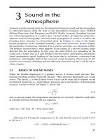
If the maximum negative value of ∆f is less than f
T
− f
m
, then positive and nega-
tive Doppler shifts are then easily identied by looking at only the positive frequency
part of the spectrum, as shown in Figure 6.1.
The frequency f
T
sine wave generator is usually continuously running, but its
output is switched to the speaker during the transmitted pulse. This is a very con-
venient signal to use as the mixing signal, so that f
m
= f
0
. However, since cos(2π∆ft)
= cos(2π[−∆f]t), positive and negative Doppler shifts cannot be distinguished. This
means that, say, easterly and westerly winds will give the same result. To overcome

this limitation, a quadrature, or 90° phase, signal is also mixed with the echo signal
Mt ft
QT



22cos P
giving
3588_C006.indd 158 11/20/07 4:18:11 PM
© 2008 by Taylor & Francis Group, LLC
SODAR Signal Analysis 159
It A ft
Qt A ft








cos
sin
2
2
PJ
PJ
$
$
(6.4)

This in-phase and quadrature-phase pair allows the amplitude, phase, and Dop-
pler shift to be determined since
It jQt Ae
jft







2PJ$
and the Fourier spectrum of this combination has either a single positive peak (for ∆f
positive, or a single negative peak (for ∆f negative). Generation of a quadrature, cosine,
signal at frequency f
T
is generally a simple hardware task. The echo signal does need
to be passed through two mixing circuits and sampled with two ADC channels.
The Doppler shift from a 20 m s
–1
horizontal wind is 64 Hz for a 1.6-kHz
SODAR, 180 Hz for a 4.5-kHz system, and 230 Hz for a 6-kHz system. It is nec
-
essary to sample at least twice the highest frequency, and depending on BP lter
characteristics, perhaps three or four times the highest frequency. For example, the
AeroVironment 4000 typically samples at 960 Hz, giving 960 s
–1
×400m/340ms
–1
= 1130 samples for a height range of 200 m. In practice SODAR systems will usu-

ally sample a little longer than for the range displayed or recorded, to avoid combin-
ing echoes from more than one pulse. This also affords the opportunity to measure
the background noise during the period at the top of the range in which no echoes
are being returned. The total number of samples per pulse is not large, and so can
be stored pending Fourier transforming. The fast Fourier transform (FFT) can be
0
Positive Doppler shift
f
T
– f
m
–(f
T
– f
m
) f
T
– f
m
0
∆f
∆f
Negative Doppler shift
FIGURE 6.1 Positive and negative Doppler shifts are readily distinguished providing
f
T
−f
m
−|∆f| > 0.
3588_C006.indd 159 11/20/07 4:18:15 PM

© 2008 by Taylor & Francis Group, LLC
160 Atmospheric Acoustic Remote Sensing
completed on sequential groups of samples, corresponding to the displayed range
gate length, or from overlapped groups of samples so that more spectra can be dis-
played (although not with additional information). FFTs are most conveniently per-
formed on groups of 2
n
samples; 64 samples at 960 samples per second gives a range
gate of 64 ì 340/(2 ì 960) = 11 m, but the AeroVironment reports Doppler spectra at
every 5 m (i.e., uses
overlapped groups of samples for FFTs).
6.1.4 WINDOWING AND SIGNAL MODULATION
Sampling a nite length of the time series record, for the purposes of doing an FFT,
is equivalent to sampling the entire time series and then multiplying the series of
samples by a rectangular function of duration N/f
s
where N is the number of samples
in the FFT. The effect of this is to convolve the power spectrum of the time series
with a sin(Nf/f
s
)/(Nf/f
s
) function. The spectral peak level from a single sine compo-
nent will vary in value depending on what frequency the peak is at.
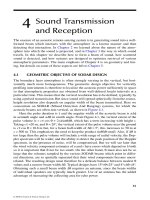
The four plots in Figure 6.2 show part of the positive half of a spectrum which
contained 64 points in the FFT and was sampled at 960 Hz. The top plot shows the
result (solid diamond points) for a sine wave at 97.5 Hz. Because of where the sam
-
pled points fall in relation to the peak of the sin(Nf/f
s

)/(Nf/f
s
) function, the result-
ing estimate of the peak is only 0.4 instead of 1.0. The second and third plots show
results for sine waves at frequencies of 100 and 105.5 Hz. The bottom plot shows the
result when the sampled time series has been multiplied by the Hanning window
Ht
f
N
t
s



Ô
Ư
Ơ
Ơ
Ơ
Ơ

ả
à
à
à
à
Đ
â
ă
ă

ă
ã
ạ
á
á
á
1
2
12
1
cos P
so that the sampled values always are small at the start of the sampled group and at
the end. The result of this windowing is that the spectrum for a pure sine wave is
wider (as shown in the ideal curve on the bottom plot). The worst-case position of
the spectral peak with respect to the frequency bins then gives frequency estimates
which are higher because they are on a wider curve. They are still only 0.7 instead
of 1.0, however.
Other windows can be used: all give better estimation of peak value but poorer
frequency resolution, when compared to the no-window case.
6.1.5 DYNAMIC RANGE
The amplied, ltered, and demodulated signal is an analog time series. This is fed
to an ADC. The digital bit pattern is then stored as a representation of the sampled
voltage of the SODAR signal. If the circuit has ramp gain to offset the spherical
spreading loss, and has a band-pass lter to limit the noise bandwidth, then a 10-bit
ADC is adequate. In this case, at best, the resolution is one part in 2
10
(1:1024), or
0.1%. In practice, this is far more accurate than the generally noisy input signals.
However, if no ramp gain is used, a SODAR signal could be expected to vary by at
least a factor of (320/10)

2
= 1024 between heights 10 and 320 m. If 0.1% resolution
is required at the upper height, then 20 bits are required. Thus to have a simpler
3588_C006.indd 160 11/20/07 4:18:16 PM
â 2008 by Taylor & Francis Group, LLC
SODAR Signal Analysis 161
0.0
0.2
0.4
0.6
0.8
1.0
0 50 100 150 200
Frequency (Hz)
Power Spectrum
0.0
0.2
0.4
0.6
0.8
1.0
0 50 100 150 200
Frequency (Hz)
Power Spectrum
0.0
0.2
0.4
0.6
0.8
1.0

0 50 100 150 200
Frequency (Hz)
Power Spectrum
0.0
0.2
0.4
0.6
0.8
1.0
0 50 100 150 200
Frequency (Hz)
Power Spectrum
FIGURE 6.2 The effect of the Doppler shift not being a multiple of f
s
/N.
3588_C006.indd 161 11/20/07 4:18:17 PM
© 2008 by Taylor & Francis Group, LLC
162 Atmospheric Acoustic Remote Sensing
preamplier circuit, the ADC bit width should be preferably 24 bits so as to have
sufcient dynamic range.
Once the FFTs have been performed, spectral peak detection methods are used
to determine velocity components and the raw samples are usually discarded. Note
that sampling at, say, 960 samples per second gives turbulence samples every 0.18 m,
which is much smaller than the real spatial resolution for turbulence. Consequently,
some averaging, say to 5 m (~30 samples) is usual, and only the averages are stored.
Such averaging will normally be done in log space (dB values are averaged).
6.2 DETECTING SIGNALS IN NOISE
Reasonable wind estimates can be made in noisy conditions in which the power SNR
is less than 1. The signal peak needs to be detected, however, by some characteristic
which distinguishes it from the noise. Such characteristics include the following.

6.2.1 HEIGHT OF THE PEAK ABOVE A NOISE THRESHOLD
Background noise can be estimated within a power spectrum from the highest fre-
quency parts of the spectrum, since the spectrum is usually considerably wider than
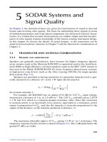
necessary for typical winds. For example, the noisy spectrum in Figure 6.3 has a sig
-
nal peak at 100 Hz, and the peak at that frequency is a likely candidate because of its
width and height. The noise threshold might have been set at say 1.0 based on noise
levels from 300 to 480 Hz, but in this example this still leaves two possible peaks.
6.2.2 CONSTANCY OVER SEVERAL SPECTRA
Most commonly, averaging of power spectra is used to improve SNR. Averaging can-
not be done on the time series, since this has positive and negative voltages and the
phase is random, so any averaging reduces the signal component as well as the noise.
But the power series is the square of the absolute value of the Fourier spectrum, and
all phase information is therefore removed. Averaging the signal component does not
Frequency (Hz)
0.0
0.5
1.0
1.5
2.0
0 100 200 300 400
Power Spectrum
FIGURE 6.3 Threshold detection of possible signal peaks.
3588_C006.indd 162 11/20/07 4:18:18 PM
© 2008 by Taylor & Francis Group, LLC
SODAR Signal Analysis 163
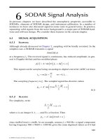
change it, but averaging the noise component, which is random, reduces its uctua-
tions by the square root of the number of spectra in the average (see Figure 6.4).
For example, the AeroVironment 4000 typically records spectra at a particular
range gate every 4 s, but displays data every ve minutes. This means that 75 spectra

are averaged. Taking the above example, and averaging successive spectra, gives the
solid curve in Figure 6.4.
The peak position is often estimated from the average frequency in the spectrum
(Neff, 1988):
ˆ
f
fP f df
Pfdf
R
R



°
°
(6.5)
but this should only be applied to the full, double-sided, spectrum.
6.2.3 NOT GENERALLY BEING AT ZERO FREQUENCY
In many circumstances it is known that there is some wind, and therefore any peak at zero
frequency must be from a xed echo. This part of the spectrum can then be ignored.
6.2.4 SHAPE
The spectrum shape for the signal component is often known from considerations of
pulse length, etc. One way of discriminating against noise is to successively t this
shape with its peak at each spectral bin, and accept the position giving the best t. A
good approximation is a Gaussian, or even a parabola of the right width.
An even simpler variant is to take a weighted sum of several spectral bin values,
and accept the position giving the highest sum. The weights can be all unity (search-
ing for maximum power in a given signal BW), or reect the expected shape of the
signal peak.
Frequency (Hz)

0.0
0.5
1.0
1.5
2.0
2.5
3.0
0 100 200 300 400
Power Spectrum
FIGURE 6.4 The effect of averaging the power spectrum shown in Figure 6.3.
3588_C006.indd 163 11/20/07 4:18:20 PM
© 2008 by Taylor & Francis Group, LLC
164 Atmospheric Acoustic Remote Sensing
6.2.5 SCALING WITH TRANSMIT FREQUENCY
A much more sophisticated method is to use two or more transmit frequencies. The
Doppler shift scales with the transmit frequency, so peaks at the correct position in
the spectra from different transmit frequencies indicate a true signal. This method is
probably used by Scintec.
6.3 CONSISTENCY METHODS
Typically, the time series from a ±f
s
/2 bandwidth SODAR prole is sampled and FFTs
performed on small blocks of samples, perhaps equivalent to 5 m vertically. A spec
-
tral peak detection algorithm then nds the individual Doppler shifts at each range
gate. Velocity components are combined to give speed and direction. This results in
individual and independent estimates of velocities at a series of vertical points.
Consistency checks and smoothing algorithms are then applied. This step makes
a connection between the independent estimates (or assumes a connection). Combin-
ing velocity components may be interleaved with this check/smooth process.

Is it possible to come up with a systematic algorithm for smoothing, allowing for
poor data points, and combining several proles and points within a prole as con-
sistency checks? The following method has been described by Bradley and Hüner-
bein (2004).
A typical plot of spectra versus height shows generally higher spectral peaks
near the ground, and increasing spectral noise at higher altitudes. Examination of
plots such as Figures 6.5 and 6.6 can indicate the most likely velocity prole by fol
-
lowing the progression of spectral peaks with height.
At height z
m
(m = 1, 2, …, M), power spectral estimates P
im
= P(f
i
, z
m
) are mea-
sured at frequencies f
i
(i = 1, 2, …, I). The frequencies correspond to velocity compo-
FIGURE 6.5 Typical raw power spectra versus height.
3588_C006.indd 164 11/20/07 4:18:22 PM
© 2008 by Taylor & Francis Group, LLC
400
200
150
100
He
ight (m)

Power
Al
o
ng-
be
am

V
el
oc
it
y (m/
s
)
50
–20
–10
0
0
10
20
300
200
100
0
SODAR Signal Analysis 165
nents u
i
. Higher values of P
im

are more likely associated with the echo signal rather
than with noise. The quantity
S
im
im
P
2
1

(6.6)
therefore represents the relative uncertainty of a particular f
i
being at the signal peak
for height z
m
. We therefore treat the f
i
, or equivalently the corresponding u
i
, as mea-
surements of signal peak position made with variance
S
im
2
.
Assume that the u are a linear function of basis functions K(z) with unknown
coefcients x as follows.
u = Kx + F (6.7)
This puts the problem into the context of the solution of a set of linear equations.
In particular, use of constraints, such as smoothness, prole rate of change, limiting

the deviation from other data points, etc., can be applied by calling upon the huge
constrained linear inversion literature.
There are still a number of arbitrary decisions required, however. These include
1. The relationship between the power spectral estimates and the variance,
2. The choice of basis functions, and
3. How to include other prole data as constraints.
Other possible relationships between P
im
and
S
im
2
include
The peak is the most likely estimator:
S
N
im
im
P
2
1

200
180
160
140
120
100
Height (m)
80

60
40
20
–15 –10 –5 0
Along-beam Velocity (m/s)
51015
FIGURE 6.6 The spectra of Figure 6.5 shown as a contour plot.
3588_C006.indd 165 11/20/07 4:18:27 PM
© 2008 by Taylor & Francis Group, LLC
166 Atmospheric Acoustic Remote Sensing
The center of a wider peak is a good estimator:
S
N
N
im
m
i
i
P
2
2
2
1



£
A t to the peak gives the best estimator:
S
NN

N
im m i
I
PPuu
2
2
1


§
©
¨
·
¹
¸

£
,
One example of basis function is a Gaussian
Kz e
n
z
zz
z
n




1

1
2
2
2
S
S
(6.8)
Figure 6.7 shows a typical t using this method, but without any constraints from
other proles. The method appears to show promise.
6.4 TURBULENT INTENSITIES
There are two basic requirements in obtaining meaningful turbulent intensities:
1. Calibration of the system variable part of the SODAR equation and
2. Allowing for the background noise.
Calibration is actually quite difcult. One can try putting some well-dened
scattering object above the SODAR, but this must be above the reverberation part
200
180
160
140
120
100
Height (m)
80
60
40
20
–15 –10 –5 0
Along-beam Velocity (m/s)
51015
FIGURE 6.7 The t through the spectra (white line) to give the spectral peak at each height.

A Gaussian constraint is used for smoothness of velocity variations in the vertical.
3588_C006.indd 166 11/20/07 4:18:32 PM
© 2008 by Taylor & Francis Group, LLC
SODAR Signal Analysis 167
of the SODAR range (i.e., above 20 m or so) and must be in the main beam of the
SODAR (i.e., at 20 m the object must be located to within ±1 or 2 m horizontally).
This is quite difcult with a tethered balloon, for example, but it might be possible to
use an object on an overhead wire. Alternatively, a sonic anemometer can be used,
providing one can work out how to extract meaningful records from it, and then
allow for the extra vertical distance to the rst usable SODAR range gate.
Background noise, P
N
, can be allowed for using the turbulence or spectrum lev-
els recorded from the highest one or two range gates, or from receiving without
transmitting for a while, or from the wings of the power spectra. Then
C
PP
xPGAcf
e
z
T
N
Te T
z
2
4
2
3
1
3

2
310


§
©
¨
¨
¨
·
¹
¸
¸
¸


T
A
222
T
§
©
¨
¨
¨
·
¹
¸
¸
¸

(6.9)
If calibrated turbulence levels are required, care must also be exercised that xed
echoes are not contaminating the time series record. Gross xed echoes are always
evident on the SODAR facsimile display, but there is a problem with part contami-
nation. So it is a good idea to look at the spectra on either side of a
C
T
2
estimate, to
see if there is a signicant peak at zero frequency. The true signal spectral peak is
of course also a measure of
C
T
2
, but this will be only available at the vertical spatial
resolution of the winds, rather than the vertical spatial resolution of the turbulence:
this reduced resolution may be adequate in many cases however.
C
V
2
measures derived from SODAR winds should be treated with caution: they
will usually be only an approximation to the true values since assumptions are nec-
essary on homogeneity and Taylor’s “frozen eld” hypothesis.
6.4.1 SECOND MOMENT DATA
SODARs record T
u
, T
v
, and T
w

, the standard deviations of wind speed components.
These standard deviations are useful as
1. An indicator of variability of winds (and likely uncertainties in
u, v, and w),
2. Statistic variables to obtain other quantities such as wind energy, and
3. Input into similarity relationships to derive other quantities.
The latter is useful in, for example, obtaining estimates of surface heat ux, H,
in convective conditions through (Weill et al. 1980)
S
w
z
M
H
T
3

(6.10)
where M is a constant and T is absolute temperature. Also, the mixing layer height,
Z
m
, can be estimated through (Asimakopoulos et al., 2002)
d
dz
z
Z
wm
S
2
0
32

at
.
(6.11)
3588_C006.indd 167 11/20/07 4:18:38 PM
© 2008 by Taylor & Francis Group, LLC
168 Atmospheric Acoustic Remote Sensing
6.5 PEAK DETECTION METHODS OF
AEROVIRONMENT AND METEK
The SODAR incorporates signal-processing software to determine
1. The position in the spectrum of the signal peak (corresponding to Doppler
shift) and
2. The averages over a number of proles (to improve SNR).
The methods for achieving these tasks vary a little between manufacturers.
Some examples follow.
6.5.1 AEROVIRONMENT
The AeroVironment system performs peak detection on each individual 64-point
spectrum (128-point spectra can also be user-selected). This is done by nding the
highest power in any contiguous 5-spectral-point group (or 7-point for a 128-point
spectrum) across the frequency spectrum. The SNR is then dened as the 5-point
power divided by the power in the remaining 59 points normalized by multiplying
by 59/5. Finally, averaging the accepted peak positions over N
s
proles gives the
estimated Doppler shift for the particular range gate and beam. Note that if the user
selects the option to use beam 3 data, then a rejected beam 3 spectrum causes the
beam 1 and beam 2 peak estimates to also be rejected at that range gate for that pro-
le (i.e., the system does not default to a 2-beam conguration which might give aver-
ages of mixed 2-beam and 3-beam calculations). Numbers of accepted beam 1, beam
2, and beam 3 peak estimates in each averaging interval are output for the user.
The system also employs an adaptive noise threshold as part of the decision to

accept/reject a spectrum. This threshold is determined by sampling the background
noise prior to the transmit pulse, and appropriately scaling this threshold to account
for spherical beam divergence with altitude. This option can be disabled or enabled
by the user. If this option is disabled, the system uses a xed noise threshold which
is applied at every altitude.
Statistical analysis shows that the uncertainty in each estimate of the position of
the spectral peak in this scheme depends on
()SNR
f
f
1
$
S
¤
¦
¥
¥
¥
¥
´
¶
µ
µ
µ
µ
µ
.
6.5.2 METEK
Metek average N
s

spectra for each beam and each range gate. Each recorded value
in a spectrum is the sum (P
A
+ P
N
) of the echo P
A
from atmospheric turbulence and
the Gaussian noise P
N
which has zero mean and variance. The SNR from a single
spectral estimate is
SN R
P
A
P
1

S
3588_C006.indd 168 11/20/07 4:18:40 PM
© 2008 by Taylor & Francis Group, LLC
SODAR Signal Analysis 169
If N
s
spectra are averaged, the average spectral estimate becomes
P
N
P
A
s

N
N
s

£
1
1
,
and the variance in this estimate is var
11
1
2
N
P
N
s
N
N
s
P
s
£
¤
¦
¥
¥
¥
¥
¥
´

¶
µ
µ
µ
µ
µ
µ
S. The SNR is therefore
SN R N
P
Ns
A
P
s

S
(6.12)
In the Metek SODAR, 32 complex Fourier amplitudes are obtained over N
s
= 20 to
60 proles, giving 32 averaged spectral intensities. Two noise spectra measurements
are made shortly before each pulse is transmitted and these are averaged to obtain
an estimate of P
N
at each frequency in the Fourier spectrum. These averaged noise
intensities are subtracted from the averaged intensities received after the pulse, to
give residual power spectra at each range gate. It is assumed that the noise-free signal
power spectrum has a Gaussian shape
Pf
e

f
ff
f
0
1
2
2
2
$
PS
S


¤
¦
¥
¥
¥
¥
¥
´
¶
µ
µ
µ
µ
µ
µ
ˆ
where

$f
T

1
is the frequency resolution. If logarithms of the spectral estimates
are used,
ln
ˆ
Pf f f
f
f
0
2
1
2
$
PS
S
¤
¦
¥
¥
¥
¥
¥
´
¶
µ
µ
µ

µ
µ
µ


¤
¦
¥
¥
¥
¥
´
¶
µ
µµ
µ
µ
µ
2
(6.13)
is a quadratic in f. Using least-squares, the moments P
0
,
ˆ
f
, and T
f
can be estimated.
In practice, only n spectral points within 1/4 height (6 dB) of the main peak are
included in the least-squares t. Simulations based on this scheme show that, for

high SNR and with N
s
> 40, the uncertainty in the peak position
ˆ
f
is about 0.06
spectral bin widths and the uncertainty in T
f
is about 0.2 spectral bins. If all cases
are rejected which have SNR below a certain critical threshold, then this accuracy
is expected. With %z = 20 m and f
T
= 1675 Hz, the error in the radial velocity com-
ponent is
SS
v
f
r
z

ˆ
.$ 01
1
ms
and the error in the estimate of the width of the
velocity spectrum is 0.17 m s
–1
. For a tilt angle of R = 20°, and given that the two
horizontal velocity components are generally comparable and dominate over the ver-
tical component,

S
S
J
V
v
r
y
2
04
sin
.ms
–1
.
Similar analysis gives the uncertainty T
Z
in the wind direction as about 6° for V =
5ms
–1
.
3588_C006.indd 169 11/20/07 4:18:50 PM
© 2008 by Taylor & Francis Group, LLC
170 Atmospheric Acoustic Remote Sensing
6.6 ROBUST ESTIMATION OF DOPPLER
SHIFTFROM SODARSPECTRA
6.6.1 F
ITTING TO THE SPECTRAL PEAK
Assume that a sinusoidal signal s(t) of duration U is transmitted. The amplitude spec-
trum of the received voltage is
VVE
iii

y
(6.14)
where
V
i
is the received scattered signal component and E
i
arises from random
noise. For Gaussian-distributed E
i
, the probability of recording a spectral amplitude
magnitude between and VVdV
iii
and  is
pV dV e
i
i
E
VV
ii
E




¤
¦
¥
¥
¥

¥
¥
¥
¥
¥
´
¶
µ
µ
µ
µ
µ
µ
1
2
1
2
PS
S
µµ
µ
µ
µ
2
dV
i
(6.15)
where
m
E

2
is the variance of E
i
. The power spectral estimate at f
i
is
PVV V
iii i


2
so
pP pV
dV
dP
P
e
ii
i
i
iE
PV
ii
E







¤
¦
¥
¥
¥
¥
1
22
1
2
PS
S
¥¥
¥
¥
´
¶
µ
µ
µ
µ
µ
µ
µ
µ
2
(6.16)
From this probability distribution, the mean power spectral value at frequency
f
i

is
PPpPdP Ve
iiii
E
i
VV
ii
E



c


¤
¦
¥
¥
¥
¥
¥
°
0
2
1
2
1
2PS
S
¥¥

¥
´
¶
µ
µ
µ
µ
µ
µ
µ
µ
c
c
°

2
2
2
dV V
ii E
S
(6.17)
In other words, there is a systematic overestimate of the power spectral value by
the noise power quantity
N
E
S
2
(6.18)
Consequently, we subtract from the spectrum an estimate,

ˆ
N , of the mean power
level when no signal is present (i.e., from the highest range gates) giving a reduced
power spectrum
`
PPN
ii
ˆ
(6.19)
3588_C006.indd 170 11/20/07 4:19:01 PM
© 2008 by Taylor & Francis Group, LLC
SODAR Signal Analysis 171
The moments of are
ˆ
ˆ
NN
N
NN
N
fav

S
2
2
3
(6.20)
where N
av
are the number of spectra which are averaged to obtain
ˆ

N
.
This results in moments
`

 
¤
¦
¥
¥
¥
´
`
PPNV
NV N
ii i
PP
N
i
ii
ˆ
ˆ
2
222
2
22SSS
¶¶
µ
µ
µ

µ
y
`


3
22
2
N
NN
NP N
fav
i
(6.21)
Various pulse envelope shapes are used, but all allow
`
P
i
to be represented in the
form
`
y


PPe
i
ff
f
iD
max

1
2
2
2
S
(6.22)
Then
ln ln
max
P
P
f
P
P
ref
i
D
f
ref
`

¤
¦
¥
¥
¥
¥
¥
´
¶

µ
µ
µ
µ
µ
µ
2
2
2S

¤
¦
¥
¥
¥
¥
¥
´
¶
µ
µ
µ
µ
µ
µ

¤
¦
¥
¥

¥
¥
¥
´
¶
µ
µ
µ
f
f
D
f
i
f
SS
22
1
2
µµ
µ
µ
f
i
2
(6.23)
where P
ref
is a reference value (for example, 1 V
2
). In other words, the logarithm of

the reduced power spectrum has a quadratic dependence on frequency.
We nd the nearest spectral frequency to the peak position, and write the index
i relative to this, so the nearest spectral frequency to the peak is labeled f
0
. Least-
squares is used to estimate the three coefcients of the quadratic using 2Q+1 points
centered around f
0
(typically Q = 2 or 3). We use an odd number of tting points
because in the case of unweighted least-squares this leads to simplication.
We now apply the above methods to raw spectral data recorded from a Metek
SODAR/RASS. The relevant parameters are given in Table 6.1. The time-series
echo strength is recorded for 3.2 s and each range gate (region over which each spec
-
trum is valid) is 16 m in vertical extent. The atmospheric conditions were low wind
and fairly neutral conditions (so relatively weak reections) but with low levels of
external background acoustic noise.
Figure 6.8 shows a typical Hanning-windowed time series for one range gate.
Figure 6.9 shows the corresponding amplitude spectrum. Note the signal peak near
the transmitting frequency. From such spectra more localized spectra are selected,
so that only possible Doppler shifts are included in the analysis. For a beam tilt angle
of 20°, the radial velocity component for a horizontal wind of 20 m s
–1
will give a
3588_C006.indd 171 11/20/07 4:19:07 PM
© 2008 by Taylor & Francis Group, LLC
172 Atmospheric Acoustic Remote Sensing
TABLE 6.1
List of parameters for the Metek SODAR
Parameter Description Value

f
T
(Hz) Transmitted frequency 1674
Us
Pulse duration 0.0958
f
s
(Hz) Sampling frequency 44100
N
f
Number of spectral estimates 4096
%f (Hz)
Frequency interval in spectrum 10.8
–0.10
–0.08
–0.06
–0.04
–0.02
0.00
0.02
0.04
0.06
0.08
0.10
1.10 1.12 1.14 1.16 1.18 1.20
1.22
Time (s)
Signal (V)
FIGURE 6.8 A typical Hanning-windowed time series for one range gate from the
Metek SODAR.

FIGURE 6.9 The spectrum for a single range gate Hanning-windowed time series.
3588_C006.indd 172 11/20/07 4:19:08 PM
© 2008 by Taylor & Francis Group, LLC
0
2
4
6
8
10
12
14
16
0 500 1000 1500 2000 2500
Frequency (Hz)
Amplitude Spectrum
SODAR Signal Analysis 173
Doppler shift of 67 Hz, so considering 16 spectral frequencies over the range 1593
to 1755 Hz should sufce for this data set. Figure 6.10 shows a power spectrum (P
i
values) from the range gate centered at 197 m. Estimation of SNR using the wings
of the spectrum around the peak value gives SNR = 8 dB. In Figure 6.11 the data
values for the quadratic t are shown. The estimated value for peak frequency is f
D
=1681±2 Hz and for width T
f
= 9.7±0.9 Hz.
0
10
20
30

40
50
60
70
80
90
1580 1630 1680
1730
Power Spectrum
FIGURE 6.10 A local spectrum taken from range gate 13 (height 197 m) and for which the
estimated SNR is 8 dB.
FIGURE 6.11 Plot of log-corrected power spectrum from data in Figure 6.10 and with
Q = 3. Data are shown with dark dots and the t with a solid line.
3588_C006.indd 173 11/20/07 4:19:10 PM
© 2008 by Taylor & Francis Group, LLC
–6
–4
–2
0
2
4
6
1640 1650 1660 1670 1680 1690 1700 1710 1720
Frequency (Hz)
ln(P
ref
/P´)
174 Atmospheric Acoustic Remote Sensing
6.6.2 ESTIMATION OF T
W

In practice reections are from an ensemble of scatterers which provide a continuum
of Doppler shifts. This gives spread to the Doppler spectrum which is particularly
important for vertical proling since the variance, S
w
2
, in vertical velocity is an
important boundary layer parameter.
Assume that the Doppler frequency from the ensemble has a Gaussian probability
centered on
f
D
and with standard deviation T
D
. This range of Doppler frequencies will
cause spectral broadening of the signal, and estimation of this extra broadening from
a vertical beam provides useful insights into turbulent eddy dissipation rates through
the standard deviation in vertical velocity, T
w
. A typical value for T
w
is 0.3 m s
1
, giv-
ing T
D
= 8 Hz for a 4500-Hz SODAR system (i.e., comparable with T
f
).
Each scatterer in the ensemble contributes a power spectrum which may be
approximated by a Gaussian, so that the total spectrum is

`


Đ
â


Ô
Ư
Ơ
Ơ
Ơ
Ơ
Ơ

ả
à
à
à
à
à
à
Pf Pe
D
ff
D
f
1
2
1

2
2
PS
S
max
ăă
ă
ă
ă
ă
ã
ạ
á
á
á
á
á


Ô
Ư
Ơ
Ơ
Ơ
Ơ
Ơ

ả
à
à

à
à
à
à
edf
ff
D
DD
D
1
2
2
S
c
c


Ô
Ư
Ơ
Ơ
Ơ
Ơ
Ơ

ả
à
à
à
à

à
à


P
e
f
T
ff
D
T
max
S
S
S
1
2
2
(6.24)
which has a variance, SSS
TfD
222
, equal to the sum of the contributing variances,
as expected. There is now an extra variability (in addition to the background noise
discussed above) given by
S
PS
S
`

Ô
Ư
Ơ
Ơ
Ơ
Ơ
Ơ

ả
à
à
à
à
à
à

Đ
â
ă
P
D
ff
Pe
D
f
2
1
2
1

2
2
max
ăă
ă
ă
ă
ã
ạ
á
á
á
á
á


Ô
Ư
Ơ
Ơ
Ơ
Ơ
Ơ

ả
à
à
à
à
à

à
2
1
2
2
edf
ff
D
DD
D
S
c
c


`
P
2
or
S
S
S
S
S
S
SSS
`


`

P
D
f
D
f
f
P
e
D
fDT
2
2
2
2
2
2
2
1
1
2
2
222



f
D

2
1
(6.25)
The maximum relative variation due to the spread in Doppler shifts is therefore
SA
A
`
`




P
P
2
2
1
12
1
max
(6.26)
where
A
S
S

D
f
2
2

.
3588_C006.indd 174 11/20/07 4:19:18 PM
â 2008 by Taylor & Francis Group, LLC
SODAR Signal Analysis 175
The regression methods discussed above can be used to estimate
SSS
TfD
222

and hence T
D
since
S
f
2
is known from the system design. The relative error in esti-
mated T
D
is
S
S
S
SS S
S
S
S
SS S
DT T
D
Tf f

T
T




22 2
2
1
1
(6.27)
If
SS
Df
22

there is a large relative error multiplication factor in (6.27). Fig-
ure 6.12 shows the relative error in
T
w
as a function of T
w
for several values of SNR
and
f
T
f
S
.
This emphasizes the importance of having good SNR for T

w
estimates, as well as
the preference of a long pulse (small T
f
). Higher frequency SODARs also do better.
A value of
f
T
f
S
170
corresponds approximately to a 1700 Hz SODAR having a 0.05-s pulse. For large
T
w
,
the relative error asymptotically approaches
S
S
S
T
T
.
6.7 AVERAGING TO IMPROVE SNR
The time series from successive proles should not be averaged, since they are inco-
herent and will average toward zero.
Averaging of power spectra from successive proles is useful, since phase
information has been removed. The noise power uctuates more than the signal,




        

w





w

w
FIGURE 6.12 Relative error in sigma-w value. Five-point ts with peak at a spectrum fre-
quency. SNR = 20 dB, f
T
/T
f
= 170 (plus signs); SNR = 20 dB, f
T
/T
f
= 340 (circles); SNR =
10 dB, f
T
/T
f
= 170 (triangles); SNR = 10 dB, f
T
/T
f
= 340 (crosses).

3588_C006.indd 175 11/20/07 4:19:25 PM
© 2008 by Taylor & Francis Group, LLC
176 Atmospheric Acoustic Remote Sensing
providing the averaging time is not too long (say no longer than 20 minutes, but this
signal autocorrelation time will depend on the environment). Noise powers
P
N
i
from
the ith prole, at a particular range gate, are summed in the averaging process
P
n
P
NN
i
n
i


£
1
1
(6.28)
and
SSS
av
N
N
P
i

n
P
P
P
i
N
i
N
2
2
2
1
2
1

t
t
¤
¦
¥
¥
¥
¥
¥
´
¶
µ
µ
µ
µ

µ


£
nnn
i
n
P
N
¤
¦
¥
¥
¥
¥
´
¶
µ
µ
µ
µ


£
2
1
2
S
(6.29)
so the standard deviation of the noise goes down as the square root of the number

of averages.
6.7.1 VARIANCE IN WIND SPEED AND DIRECTION OVER ONE AVERAGING PERIOD
Generally wind data from a number of proles are averaged. In the following we will
restrict attention to the horizontal wind components. The ith prole may contain an
acceptable u
i
wind component and/or an acceptable v
i
component. This results, after
an averaging period, in N
u
east-west components and N
v
north-south components.
The means and variances from a single averaging period are
u
N
u
N
uu
N
u
u
i
i
N
u
u
i
i

N
u
i
i
uu




££
111
1
2
2
1
2
1
S
NN
v
i
i
N
v
v
i
i
N
u
vv

u
v
N
v
N
vv
£
££





2
1
22
1
2
11
S
(6.30)
Some analysis is needed because some SODAR software gives
uv
uv
,, , ,SS
and
the mean speed
V
and direction Y, but not the errors
SS

Y
V
or
.
The wind speed V
i
can only be calculated from those N
V
proles where both u
i
and v
i
are available so N
V
≤ N
u
, N
V
≤ N
v
. Also
Vuv
u
v
iii
i
i
i





22
1
2
1
9 tan
(6.31)
Note that the wind direction needs to be calculated using four quadrants. The
average wind speed and variance in wind speed are just found in the usual way
V
N
uv
N
uv
V
ii
i
N
V
V
ii
i
N
VV






£
11
22
1
2
1
222
1
S
££


V
2
(6.32)
3588_C006.indd 176 11/20/07 4:19:35 PM
© 2008 by Taylor & Francis Group, LLC
SODAR Signal Analysis 177
or
SS S
V
u
V
u
v
V
v
N
N
u

N
N
v
22
2
2
2
y

Đ
â
ă
ă
ã
ạ
á
á


Đ
â
ă
ă
ã
ạ
áá
á


V

2
(6.33)
Also,
S
S
SS
V
V
V
u
V
u
v
V
v
N
N
N
u
N
N
v
2
2
2
2
2
2
2
y

Đ
â
ă
ă
ã
ạ
á
á


Đ
â
ă
ă
ã
ạ
á
á


22
1
N
V
V
(6.34)
is the variance in the mean wind speed over the averaging period.
The direction needs to be found from the accumulated wind runs in each com-
ponent, since otherwise averaging could result in a nearly 0 direction being inter-

preted as nearly 180. So
Yy

tan
1
u
v
(6.35)
This is why, for the AeroVironment SODAR, no number of recorded values is
given for the direction.
The variance in direction is
S
Y
S
Y
Y
2
2
2
1

t
t
Ô
Ư
Ơ
Ơ
Ơ
Ơ

ả
à
à
à
à

t
t
Ô
Ư
Ơ
Ơ
Ơ
Ơ

Ê
uv
i
u
i
N
i
u

ả
à
à
à
à

t
t

Ô
Ư
Ơ
Ơ
Ơ
Ơ

ả
à

Ê
2
2
1
2
1
1
S
Y
Y
v
i
N
i
v
u
tan

tan
àà
à
à
à

t
t

Ô
Ư
Ơ
Ơ
Ơ
Ơ

ả
à
à
à

Ê
2
2
1
2
1
1
S
Y

Y
u
i
N
i
u
v
tan
tan
àà
à





Ô
Ư
Ơ
Ơ
Ơ
Ơ
Ơ
Ơ

ả
à
à
à
à

à
à

Ê
2
1
2
22
S
i
N
v
v
uv
àà
à


Ô
Ư
Ơ
Ơ
Ơ
Ơ

ả
à
à
à
à

Đ
â
2
2
22
2
1
Nv
NN
Nu
Nv
v
uu vv
u
v
SS
ăă
ă
ă
ã
ạ
á
á
á




N
N

N
N
Nv
u
v
u
u
v
v
v
SSY
Y
222
2
2
1
tan
tan
ĐĐ
â
ă
ã
ạ
á
2
(6.36)
6.7.2 COMBINING WIND DATA FROM A NUMBER OF AVERAGING PERIODS
For wind speed S, and wind direction Z,
Suv
22

(6.37)
Y

tan
1
u
v
(6.38)
3588_C006.indd 177 11/20/07 4:19:42 PM
â 2008 by Taylor & Francis Group, LLC
178 Atmospheric Acoustic Remote Sensing
where u and v are the vector components.
We assume there are measurements u
i
, v
i
, i=1,2, , N from N proles, where the
u
i
and v
i
are measured with individual uncertainties SS
uv
ii
and . Assume that these
uncertainties arise from taking the mean of n
u
i
values of u, and n
v

i
values of v, each
with variance S
1
2
, so that
S
S
u
u
i
i
n
2
1
2

(6.39)
S
S
v
v
i
i
n
2
1
2

(6.40)

where
S
1
2
arises from error in estimating the position of the spectral peak at each
range gate, and is essentially the same for each estimation.
Now
SS
S
i
i
u
i
i
ii
S
u
S
v
2
2
2

t
t
Ô
Ư
Ơ
Ơ
Ơ

Ơ

ả
à
à
à
à

t
t
Ô
Ư
Ơ
Ơ
Ơ
Ơ

ả
àà
à
à
à

Ô
Ư
Ơ
Ơ
Ơ
Ơ

ả
à
à
à
à

Ô
Ư
2
2
2
11
S
v
u
i
iv
i
i
i
ii
n
u
Sn
v
S
ƠƠ
Ơ
Ơ
Ơ

ả
à
à
à
à
Đ
â
ă
ă
ă
ã
ạ
á
á
á

2
1
2
1
2
S
S
A
i
(6.41)
is the variance of a single S
i
, and

S
Y
S
Y
Y
ii
i
i
u
i
i
uv
2
2
2

t
t
Ô
Ư
Ơ
Ơ
Ơ
Ơ

ả
à
à
à
à

t
t
Ô
Ư
Ơ
Ơ
Ơ
Ơ

ả
àà
à
à
à

Ô
Ư
Ơ
Ơ
Ơ
Ơ

ả
à
à
à
à
à

2
2
2
2
11
S
v
u
i
i
v
i
i
i
ii
n
v
S
n
u
S
22
2
1
2
1
2
Ô
Ư
Ơ

Ơ
Ơ
Ơ

ả
à
à
à
à
à
Đ
â
ă
ă
ă
ă
ã
ạ
á
á
á
á

S
S
B
i
(6.42)
is the variance of a single Z
i

.
The mean
S and Y
are required over the N measurements, allowing for the vari-
able uncertainties. These means are found by following the usual procedures for
modeling y = a + bx, but here we have only one parameter
ay , so the one-param-
eter weighted least-squares t has the form
yy
.
The single parameter,
y
, is found by minimizing
3588_C006.indd 178 11/20/07 4:19:53 PM
â 2008 by Taylor & Francis Group, LLC
SODAR Signal Analysis 179
C
S
2
2


Ô
Ư
Ơ
Ơ
Ơ
Ơ
Ơ

ả
à
à
à
à
à
Ê
yy
i
i
i
(6.43)
where
S
i
2
is the variance in measurement y
i
, giving
y
y
i
i
i
i
i

Ê
Ê
1

1
2
2
S
S
(6.44)
and
S
S
y
i
i
N
N
2
2
1
1


Ê
(6.45)
In the context of wind-averaging of N=10 one-minute values, this gives
SS
i
i
ii
i

Ê
Ê
1
1
10
1
10
A
A
(6.46)
and
Y
B
B


Ê
Ê
1
1
10
1
10
i
i
ii
i
Y
(6.47)

where the weights are
A
i
u
i
iv
i
i
n
u
Sn
v
S
ii

Ô
Ư
Ơ
Ơ
Ơ
Ơ

ả
à
à
à
à

Ô
Ư

Ơ
Ơ
Ơ
Ơ

ả
à
à
11
2
àà
à
Đ
â
ă
ă
ă
ã
ạ
á
á
á

2
1
(6.48)
and
B
i
u

i
i
v
i
i
n
v
S
n
u
S
ii

Ô
Ư
Ơ
Ơ
Ơ
Ơ

ả
à
à
à
à
à

Ô
Ư
Ơ

Ơ
Ơ
Ơ

11
2
2
2
ảả
à
à
à
à
à
Đ
â
ă
ă
ă
ă
ã
ạ
á
á
á
á

2
1
(6.49)

3588_C006.indd 179 11/20/07 4:20:02 PM
â 2008 by Taylor & Francis Group, LLC
180 Atmospheric Acoustic Remote Sensing
Similar considerations can be used for any other averaged quantities.
An example taken from an AeroVironment 4000 return from 90 m with averag-
ing over 150 s, has measured values of u
i
= 3.4 m s
1
,
S
u
i
= 0.8 m s
1
,
n
u
i
= 38, v
i
=
3.7ms
1
, S
v
i
= 0.9ms
1
, and n

v
i
= 36. This gives S
i
=5.0ms
1
, Z
i
= 313, and T
1
=
5ms
1
. Then B
i
= 36 and C
i
= 920 rad
2
m
2
s
2
. This means that the standard deviation
in wind speed for this averaging period is S
S
i
= 0.83ms
1
and the standard deviation

in wind direction is S
Y
i
= 9.5.
6.7.3 DIFFERENT AVERAGING SCHEMES FOR SODAR
AND STANDARD CUP ANEMOMETERS
Cup anemometers represent one standard against which SODARs might be cali-
brated. As pointed out by Antoniou and Jứrgensen (2003) cup anemometers measure
wind run and divide by averaging time to obtain wind speed. Thus
V
T
Vdt
T
uvdt
cup
TT


11
0
22
0
(6.50)
whereas a SODAR obtains wind speed from the averaged u and the averaged v
components:
V
T
udt
T
vdt

SODAR
TT

Ô
Ư
Ơ
Ơ
Ơ
Ơ
Ơ
Ơ

ả
à
à
à
à
à
à
à
à


11
0
2
0
ÔÔ
Ư
Ơ

Ơ
Ơ
Ơ
Ơ
Ơ

ả
à
à
à
à
à
à
à
à
2
(6.51)
To allow for the sampled nature of the SODAR (a sample each prole), assume
that the wind is essentially in the +x-direction with small perturbations:
uUu
i ttit
v
i

a( )1 $$
v
i
(6.52)
3588_C006.indd 180 11/20/07 4:20:10 PM
â 2008 by Taylor & Francis Group, LLC

SODAR Signal Analysis 181
Then
V
N
Uu v
U
N
u
U
uv
U
cup i i
i
N
iii
i






Ê
1
1
2
2
2
1
22

2


Ê
Ê
y

Ô
Ư
Ơ
Ơ
Ơ
Ơ

ả
à
à
à
à
à
y
1
22
2
1
1
2
N
iii
i

N
U
N
u
U
uv
U
UU
N
u
NU
uv
i
i
N
ii
i
N



ÊÊ
11
2
1
22
1
(6.53)
and
VU

N
u
N
v
SODAR i
i
N
i
i
N

Ô
Ư
Ơ
Ơ
Ơ
Ơ
Ơ

ả
à
à
à
à
à
à


Ê
11

1
2
1
ÊÊ
ÊÊ
Ô
Ư
Ơ
Ơ
Ơ
Ơ
Ơ

ả
à
à
à
à
à
à


2
11
1
21
U
N
u
UN

u
U
i
i
N
i
i
N
ÔÔ
Ư
Ơ
Ơ
Ơ
Ơ
Ơ

ả
à
à
à
à
à
à

Ô
Ư
Ơ
Ơ
Ơ
Ơ

Ơ

ả
à
à
à
à
à
à

Ê
2
1
1
N
v
U
i
i
N
22
11
1
11
2
1
y
Ô
Ư
Ơ

Ơ
Ơ
Ơ
Ơ

ả
à
à
à
à
à

ÊÊ
U
N
u
UN
u
U
i
i
N
i
i
N
àà

Ô
Ư
Ơ

Ơ
Ơ
Ơ
Ơ

ả
à
à
à
à
à
à
Đ
â
ă
ă
ă
ă
ã
ạ
á
á
á

Ê
2
1
2
1
2

1
N
v
U
i
i
N
áá
y



ÊÊ
U
N
u
NU
uv
NU
uu
iii
i
N
i
N
i
11
2
1
2

2
22
11
2
jjij
ji
N
i
N
vv

w
ÊÊ
11
(6.54)
This gives
VV
UN
uv
cup SODAR i i
i
N
y

Đ
â
ă
ă
ă
ã

ạ
á
á
á

Ê
1
2
1
22
1
(6.55)
for large N. So V
cup
> V
SODAR
. Panofsky et al. (1977) show that
1
25
22
1
2
N
uv u
ii
i
N


y

Ê
.
where is the friction velocity, and assuming a log wind prole
U
uz
z
m


K
ln
0
3588_C006.indd 181 11/20/07 4:20:15 PM
â 2008 by Taylor & Francis Group, LLC