Heat Conduction Basic Research Part 5 ppt

Experimental and Numerical Studies of Evaporation Local Heat Transfer in Free Jet

89


d/d
i

0
0.2
0.4
0.6
0.8
1
1.2
1.4
1.6
00.511.522.533.5
Re=5859 Re=4366 Re=2732
Re=2037 Re=1521
d
i
=4mm, S=13mm

z/d
i

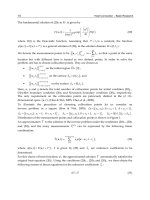
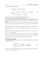
Fig. 3. Evolution of the jet diameter along the z direction.
It can be seen from figure 3 that for the same axial position (z), the jet diameter increases
with inlet Reynolds number because gravitational force increases with flow velocity and

becomes higher than surface tension force at the jet free surface. For lower Reynolds
number (Re=1521), it shows that instability starts and waves appears on the jet free
surface because capillarity force increases and becomes non-negligible compared to
gravitational force.
Along the falling jet, no evaporation has been produced and the mass flow rate is conserved.
In this case, axial distribution of the flow velocity can be deduced from the following
equation:




2
Lj
dz
mVz
4
 

(2)
At each axial position (z),


j
Vz is the average velocity of the jet,


dz is the jet diameter,
L

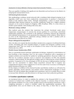
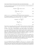
is the jet density. Figure 4 shows evolution of



jj
,inlet
Vz/V
from the injection zone to
the heat exchange surface for various inlets Reynolds numbers.
j
,inlet
V refers liquid velocity
of the jet at the nozzle exit. For each Reynolds number, velocity is high near the
impingement zone where the jet diameter is low. The free jet is accelerated after the nozzle
exit because the gravity force effect is very pronounced. After this zone, the jet velocity
decelerates quickly because liquid flow is retained on the heat exchange surface under the
effect of the capillarity force and the wall friction.

Heat Conduction – Basic Research

90
V
j
/V
j,inlet
0
1
2
3
4
5
6

00.511.522.533.5
Re=5859 Re=4366 Re=2732 Re=2037 Re=1521
d
i
=4mm, S=13mm

z/d
i
Fig. 4. Dimensionless axial velocity of the jet.
2.2 Wall parallel flow structure
Turning now to the characterisation of the local liquid layer depth near the heat exchange
surface and the velocity profile along the radial direction where the heat transfer occurs.

δ/d
i

0
0.5
1
1.5
2
2.5
-12 -8 -4 0 4 8 12
Re=3408
Re=6733
Re=2791
d
i
=2.2mm, S=95mm

r/d
i

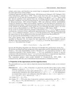
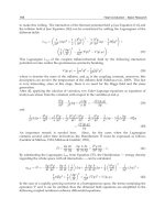
Fig. 5. Local evolution of the dimensionless liquid layer depth.
Figure 5 shows an example of the local liquid layer depth (


r

) measured for three values
of the inlet Reynolds number (Re=6733, Re=3408, and Re=2791). The nozzle diameter is of
2.2 mm for theses experiments. The jet inlet temperature is of 32°C and the nozzle-heat

Experimental and Numerical Studies of Evaporation Local Heat Transfer in Free Jet

91
exchange surface spacing is of 95 mm. Figure 5 shows three distinct zones: the impingement
zone, the zone where the liquid layer depth is approximately uniform, and the final zone
where a hydraulic jump is formed. The radius, at which the liquid layer depth increases, is
termed as the hydraulic jump radius. For higher Reynolds number, hydraulic jump is not
appeared on the heat exchange surface because it is certainly higher than the radius of the
heat exchange surface. Location of hydraulic jump on the surface is an interest physical
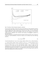
phenomenon. In the previous work, some authors (Stevens & Webb, 1992, 1993, Liu et al.
1991, 1989, Watson, 1964) show the influence of the jet mass flow rate on the hydraulic jump
radius that is defined at the radius location where the liquid layer depth attains a highest
value in the parallel flow (Figure 6a).

0
0,5
1

1,5
2
2,5
3
0 5 10 15 20 25
Rhyd
hydraulic.
j
ump
Hydraulic jump radius (R
hyd
)
Jet

r [mm]
(a)

h
y
d
i
R
d

1
10
100 1000 10000
measurements (S=40mm)
62.0
i

hyd
Re046.0
d
R

Stevens and
Webb [14]

Re
(b)
Fig. 6. a- Schematic of the hydraulic jump radius, b- Dimensionless hydraulic jump radius.

Heat Conduction – Basic Research

92
For Reynolds number ranging from 700 to 5000, Figure 6b shows dimensionless hydraulic
jump radius as a function of Reynolds number. It shows that the hydraulic jump radius
increases with the Reynolds number because flow is accelerated in the radial direction and
the hydraulic jump is moved far from the stagnation zone. The difference between the
present results and the experimental data of Stevens and Webb can be due to the uncertainty
in the data of Stevens and Webb estimated of ±0.5 cm. The present results are defined with a
maximum uncertainty of 2% and revealed an approximation dependence of the hydraulic
jump radius on the Reynolds number as
0.62
Re
:

hyd
0.62
i

R
0.046Re
d

(3)
Equation (3) estimates hydraulic jump radius with a maximum uncertainty of ±7%.
Distribution of the liquid velocity along the radial direction is determined by assuming
conservation of the mass flow rate of liquid jet. For parallel flow:





Lj
mUr2rr



(4)
Where
L

is the jet density,


j
U r is the jet average velocity in the radial direction, r is the
radial coordinate,



r is the liquid layer depth on the surface.
Figure 7 shows profiles of dimensionless velocity and shows for each inlet Reynolds
number, radial velocity profiles reaches a maximum value which is very pronounced for
higher Reynolds number.


U
j
/V
j,inlet

0
0.05
0.1
0.15
0.2
0.25
0.3
0.35
0.4
-12 -8 -
4
0
4
812
Re=6733
Re=3408
Re=2791
d
i

=2.2mm, S=95mm

r/d
i

Fig. 7. Local evolution of the dimensionless radial velocity.

Experimental and Numerical Studies of Evaporation Local Heat Transfer in Free Jet

93
 [mm]
0.0
0.2
0.4
0.6
0.8
1.0
1.2
1.4
1.6
1.8
01234567
Turbulent theory of Watson [27]
Laminar theory of Watson [27]
present results
d
i
=4mm, S=40mm, Re=4844

r/d

i

(a)
U
j
/V
j,i
0
0.5
1
1.5
2
2.5
3
01234567
Turbulent theory of Watson [27]
present results
Laminar theory of Wats on [27]
d
i
=4mm, S=40mm, Re=4844

r/d
i

(b)
Fig. 8. Comparison of the experimental results with Watson’s theory: (a) liquid layer depth
(b) dimensionless radial mean velocity.
For the same radial position, Figure 7 shows effect of the hydraulic jump on the flow
velocity. It shows that in the zone of the hydraulic jump, radial velocity is the lowest and

approximately uniform for Re=3408 and Re=2791. For all data, the maximum dimensionless
velocity is obtained for radius ranging from 2 to 4 times nozzle diameter. In the previous

Heat Conduction – Basic Research

94
work, Stevens and Webb (1989) found this maximum at r/d
i
of 2.5 for the horizontal
impinging jet on the vertical surface. Figure 7 also indicates that in the parallel flow, radial
velocity is not uniform and it is lower than inlet jet velocity at the nozzle exit. The present
results contradicts the assumption of some authors (Liu et al. 1989, Liu et al. 1991) assuming
that the flow is fully developed before the hydraulic jump, and the free surface velocity is
equal to the exit average jet velocity.
Experimental results are compared with the laminar and the turbulent theories predictions
defined by Watson (1964) in figures 8a and b. It shows that laminar theory provides the best
agreement with experimental data but sub-estimates the liquid layer depth. However, the
turbulent theory underestimates liquid velocity along the radial direction and sub-estimates
the liquid layer depth.
For all experiences showed in this section, it can be seen that when a circular liquid free jet
strikes a flat plate, it spreads radially in very thin film along the heated surface, and the
hydraulic jump that is associated with a Rayleigh-Taylor instability, can be appeared. Three
distinct regions are identified and flow velocity is varied along the jet. Therefore, local
distribution of heat flux and heat transfer coefficient is variable following the liquid layer
depth and flow velocity.
There has been little information available in the published literature on local heat
transfer for cooling using evaporation of impinging free liquid jet. The reason is that the
liquid film spreads radially on the heated surface in very thin film, and determination of
local heat flux on the wetted surface requires measurement of the temperature profiles
along the axial and radial directions without perturbing the flow. Therefore, inverse heat

conduction problem (IHCP) has been solved in order to determine locally distribution of
thermal boundary conditions at the wetted surface using only temperatures measured
inside the wall.
3. Determination of the thermal boundary conditions
In the previous work (Chen et al., 2001, Martin & Dulkravich, 1998, Louahlia-Gualous et al.,
2003, Louahlia & El Omari, 2006), IHCP is used to estimate the thermal boundary conditions
in various applications of science and engineering when direct measurements are difficult.
IHCP could determine the precise results with numerical computations and simple
instrumentation inside the wall.
In this study, experiments were investigates using a disk heated at its lower surface. The
disk is 50 mm in diameter and 8 mm thick (Figure 9). It is thermally insulated with Teflon
on all faces except the cooling face in order to prevent the heat loss. Liquid jet impactes
perpendicularly in the center of the heat exchange surface (top surface of the disk).
Temperatures inside the experimental disk are measured using 7 Chromel-Alumel
thermocouples of 200 µm diameter (uncertainty of
0.2°C). As shown in Figure 9,
thermocouples are placed at 0.6 mm below the wetted surface at radial intervals of
3.5 mm.
The experimental disk is heated continually and the wall temperatures are monitored. When
thermal steady state is reached, the heat exchange surface is quickly cooled with the liquid
jet. Time-dependent local wall temperatures are recorded, until the experimental disk
reaches a new steady state. The local surface temperature and heat flux are determined by
solving IHCP using these measurements.

Experimental and Numerical Studies of Evaporation Local Heat Transfer in Free Jet

95
r
z
E=8mm

H
meas
=7.4mm
Unknown heat flux
Insulated
R
Wetted surface
Experimental cylinder
Measured temperatures
r
z
E=8mm
H
meas
=7.4mm
Unknown heat flux
Insulated
R
Wetted surface
Experimental cylinder
Measured temperatures

Fig. 9. Physical model.
Physical model of a unsteady heat conduction process is given by the following system of
equations:

   
22
p
22

C
Tr,z,t Tr,z,t Tr,z,t Tr,z,t
1
trr
rz

 
 
 

, (4)
where 0 r R , 0
zE



T
(0,z,t) 0
r



, where
f
0tt


, 0 z E

 (5)

T
(R,z,t) 0
r



, where
f
0tt

 , 0 zE

 (6)

0
T(r,z,0) T

, where : 0 r R

 , 0 z E

 (7)

w
T
(r,E,t) Q (r,E,t)
z




, where :
f
0tt


, 0 r R

 (8)

T(r,0,t) f(r,t)

, where :
f
0tt

 , 0 r R

 (9)
Distribution of local heat flux
w
Q(r,E,t) at the heat exchange surface (z=E) is unknown. It is
estimated by solving the IHCP using temperatures
meas n n
T(r,z,t) measured at nodes (r
n
, z
n
)
inside the disk (Figure 9). Solution of the inverse problem is based on the minimization of

the residual functional defined as:


f
0
t
N
2
nn
n1
t
J(C(T), (T)) T(X ,t;C(T), (T)) f (t) dt min

  


(10)
where
nn w
T(r ,z ;Q ) are temperatures at the sensor locations computed from the direct
problem (4-9). Minimization is carried out by using conjugate gradient algorithm (Alifanov

Heat Conduction – Basic Research

96
et al., 1995). Heat flux
w
Q(r,E,t) is approximated in the form of a cubic B-spline and the
IHCP is reduced to the estimation of a vector of B-Spline parameters. Conjugate gradient
procedure is iterative. For each iteration, successive improvements of desired parameters

are built. Descent parameter is computed using a linear approximation as follows:

f
meas
f
meas
t
N
it it
nn w measnn nn w
n1
it
0
t
N
it 2
nn w
n1
0
T(r,z,t;Q ) T (r,z,t) (r,z,t;Q )dt
(r ,z ,t; Q ) dt












(11)
Variation of temperature at the sensor locations
it
nn w
(r ,z ,t; Q ) resulting from the
variation of heat flux
(, ,)
w
QrEt

is determined by solving variational problem. Variation of
functional


w
J Q resulting from temperature variation is given by:


f
meas
0
t
N
ww nnw measnn nn
n1
t
J(Q ,Q ) T(r,z,t,q ) T (r,z,t) (r,z,t)dt


  


(12)
where
it
nn w
(r ,z ,t; Q ) is determined at the sensor locations


nn
r,z
by solving variational
problem that defined by the following equations:









22
p
22
C
r,z,t r,z,t r,z,t r,z,t
1
trrrz


     
 
   
(13)
where 0 r R , 0 z E

 ,
f
0tt



(0,z,t) 0
r



, where
f
0tt

 , 0 z E

 (14)

(R,z,t) 0
r




, where
f
0tt

 , 0 z E

 (15)

(r,z,0) 0

 , where : 0 r R

 , 0 z E

 (16)

(r,E,t) 0
z





, where :
f
0tt

 , 0 r R


 (17)

(r,0,t) 0


, where :
f
0tt


, 0 r R

 (18)
3.1 Lagrangian functional and adjoint problem
Using Lagrange multiplier method, Lagrangian functional is defined as:

f
0
t
N
2
nn
n1
t
J(C(T), (T)) T(X ,t;C(T), (T)) f (t) dt min

  



Experimental and Numerical Studies of Evaporation Local Heat Transfer in Free Jet

97
+
f
t
R
2
p
2
00
TT
T
(r,z,t) r C dr dz dt
rr r z t



 



  





+


f
t
R
00
(r,t) T(r,0,t) f r,t dr dt  


f
t
E
00
T
(z,t) (R,z,t) dz dt

 



+
f
t
R
w
00
T
(r,t) (r,E,t) Q (r,E,t) dr dt
z



 




f
t
E
00
T
(z,t) (0,z,t) dz dt
r


 







RE
0
00
(r,z) T(r,z,0) T dr dz 

(19)
Let
(,,)rzt


, (,)rt

, (z,t)

, (,)zt

, (r,z)

and (,)rt

be the Lagrange multipliers.
The necessary condition of the optimization problem is obtained from the following
equation:

ww
L(Q , Q ) 0

 (20)
where
ww
L(Q , Q ) is the variation of Lagrangian functional. Equation (19) requires that all
coefficients of the temperature variation


r,z,t be equal to 0. To satisfy this condition the
necessary conditions of optimization are defined in the form of adjoint problem.




p
C
r,z,t
t





22
222
11
S(r,z,t)
rr
rrz

 



(21)
where:

meas
N
nn
n1
S(r,z,t) (r,r ;z,z )



 




nn w measnn
T(r,z,t;Q ) T (r,z,t)
,
0rR

 , 0 z E

 ,
f
0tt




(0,z,t) (0,z,t)
rr
 


, where
f
0tt

 , 0 z E


 (22)

(R,z,t) (R,z,t)
rr
 


, where
f
0tt

 , 0 z E

 (23)

f
(r,z,t ) 0


, where : 0 r R

 , 0 z E

 (24)

(r,E,t) 0
z





, where :
f
0tt

 , 0 r R

 (25)

(r,0,t) 0

 , where :
f
0tt

 , 0 r R

 (26)
where
(,,)rzt

is the Lagrange multiplier,

Heat Conduction – Basic Research

98

f
0
t

N
2
nn
n1
t
J(C(T), (T)) T(X ,t;C(T), (T)) f (t) dt min

  




is the Dirac Function,
S(r,z,t)
is the deviation between temperature measurements and
computed temperatures.
S(r,z,t) is equal to 0 everywhere in the physical domain except at
sensor locations
nn
(r ,z )
.
The Dirac function is defined by


f
0
t
N
2
nn

n1
t
J(C(T), (T)) T(X ,t;C(T), (T)) f (t) dt min

  


(27)
where
(0) 1,


0r


for r 0

and


0z


for 0z


If the direct problem and the adjoint problem are verified, variation of the Lagrangian
functional becomes:

f

t
R
ww w
00
(Q , Q ) (r,E,t) Q (r,E,t)dr dt

L
(28)
Vector gradient can be verified by the following equation:

w
Q
J' (r,E,t) (r,E,t)

 (29)
3.2 Gradient vector computation
Variation of functional


w
J Q can be approximated in the form:

ww
J(Q , Q )

f
t
ER
22
p

222
000
C
r,z,t
11
(r,z,t)dr dz dt
trrrrz




 


   


(30)
Integration by parts gives, the variation of functional becomes using Eqs (21-26):

f2
tR
ww
00
(r,t)
J(Q , Q ) (r,t) (r,t) drdt
zz

 
 





(31)

Substituting Eqs. (25) and (17) into Eq. (31),
ww
J(q , q ) becomes:
f
t
R
ww w
00
(Q , Q ) (r,E,t) Q (r,E,t)drdt 

J


ww
(Q , Q ) L (32)
Variation of functional is defined as:

Experimental and Numerical Studies of Evaporation Local Heat Transfer in Free Jet

99

f2
w
tR

ww Q w
00
J(Q , Q ) J' (r,E,t) Q (r,E,t) drdt 

(33)
Equations (32) and (33) imply that:

w
Q
J' (r,E,t) (r,E,t)

 (34)
Vector gradient can verified the following equation:

w
Q
J' (r,E,t) (r,E,t)

 (35)
3.3 Algorithm
The following iterative procedure is adopted to solve the inverse heat conduction
problem:
i.
solution of the direct problem,
ii.
calculation of the residual functional,
iii.
solution of the adjoint problem,
iv.
calculation of the components of the functional gradient,

v.
calculation of the parameter in descent direction,
vi.
calculation of the component of descent direction,
vii.
solution of the variational problem to determine the descent parameter,
viii.
the new value of the heat flux density is corrected.
If the convergence criteria is not satisfied the iterative procedure is repeated until the
functional is minimized. The minimal value of the functional depends on the temperature
measurement errors.
The direct problem, adjoint problem, and variational problem are solved using the control
volume method (Patankar, 1980) and the implicit fractional-step time scheme proposed by
(Brian, 1961).
3.4 Regularization
The inverse problem is ill-posed and numerical solution depends on the fluctuation
occurring in the measurements. The iterations are stopped at the optimal value of the
residual functional which satisfies the criteria:

f
meas
t
N
2
wnn
n1
0
1
J(Q ) (r ,z ,t) dt
2





(36)
Here,
2
nn
(r ,z ,t) is the standard deviation of measurement errors for the temperatures
measured at locations
nn
(r ,z ) .
4. Inverse estimation of the boundary conditions
4.1 Numerical verification of the solution procedure
The numerical procedure is verified by using a known heat flux varying with time and the
radius of the disk. Heat flux is imposed at the top surface of the disk (z = E) as shown in
Figure 10 by the continuous curve. The bottom surface (z=0) is assumed to be at the constant

Heat Conduction – Basic Research

100
temperature of T(r,0,t)= 40°C. For each numerical application, time step size is chosen with
respect to delta Fourier number condition defined by the following equation:


2
p
meas
t
Fo 0.001

C
EH






(37)
The delta Fourier number is based on the sensor depth, thermal characteristics of the solid,
and time step (Williams & Beck, 1995, Beck & Brown, 1996).

Q
w
[kW/m
2
]
0
0000
0
0000
0
0000
0
0000
0
0000
0
0000
0

0000
0
0000
0 0.005 0.01 0.015 0.02 0.025
r [m]
17x9 17x9
25x9 25x9
12x7 12x7
Grids:
t = 40 s
t = 15 s
200
0
400
0
600
0
800
0
1000
0
1200
0
1400
0
1600
0
Exact heat flux

Fig. 10. Heat flux variation with radius on the top surface. Verification of the IHCP: solid

line (“measurements”), symbols (“estimations using inverse method”).
In order to validate inverse estimation procedure, it is assumed that temperatures calculated
from the direct problem at the measurement points are used as the measured temperatures
(
meas n n n n n
T (r,z,t) f(r,z,t) ) for solving ICHP. Figure 10 shows that the estimated heat flux is
closed with the exact heat flux for different times. This validation is carried out for the
number of approximation parameters equal to 9x9. The maximum deviation between the
computed temperatures and the simulated measured temperatures is of 0.03°C. The
evolution of the residual functional
w
J(Q ) is a function of the number of iterations that are
continued till the convergence criteria is satisfied.
4.2 Inverse estimation of evaporation local heat transfer for jet impingement
4.2.1 Evaporation local heat transfer for unsteady state
For inlet Reynolds number of 7600, Figure 11 shows an example of temporal temperatures
measured for different radial locations at 0.6 mm below the heat exchange surface. During
experiments, heat flux imposed inside the experimental disk is 45 W, the nozzle-heat
exchange surface spacing is 30 mm, and the liquid inlet temperature is 42°C. At the steady

Experimental and Numerical Studies of Evaporation Local Heat Transfer in Free Jet

101
state, wall temperatures are 78°C. When the heat exchange surface is wetted, the wall
temperatures decrease continually and reach a stable value during a short period.
Temperature at the stagnation zone is lower than the temperature measured far from the
impingement zone. IHCP is solved using temperatures measured at H
meas
= 7.4mm (Figure
11) in order to estimate the local surface temperature and heat flux. These local thermal

characteristics are estimated using the temperatures measured at the bottom surface (z=0) as
the boundary condition to solve the direct problem.





T [°C]
Time [s]
50
55
60
65
70
75
80
0 20 40 60 80 100 120
r/R = 0.88
r/R = 0.76
r/R = 0.46
r/R = 0
Time [s]
50
55
60
65
70
75
80
0 20 40 60 80 100 120

r/R = 0.88
r/R = 0.76
r/R = 0.46
r/R = 0




Fig. 11. Temperatures measured inside the solid at z = H
meas
.
Figures 12 and 13 show, respectively, the unsteady evolution of the predicted surface heat
flux and temperature at different radial locations on the cooling surface (z = E =8 mm).
Surface temperature is low in the stagnation and in impingement zone where heat flux is
high. The difference between the wall and liquid temperatures is high at the moment when
the liquid jet impinges the heat exchange surface. After this, heat flux decreases with time
and follows the same trend for each radial location. Heat flux decreases after the
impingement zone because liquid spreads along the radial direction as a very thin film. The
experimental data for each radial location and inlet Reynolds number, follows the same
trend. For brevity, theses curves are not shown in this figure.

Heat Conduction – Basic Research

102
Q
w
[kW/m²]
Time [s]
0
20

40
60
80
100
120
140
160
180
200
0 20 40 60 80 100 120
r/R = 0
r/R = 0.118
r/R = 0.2352
r/R = 0.4704
r/R = 0.6468
r/R = 0.8232
Time [s]
0
20
40
60
80
100
120
140
160
180
200
0 20 40 60 80 100 120
r/R = 0

r/R = 0.118
r/R = 0.2352
r/R = 0.4704
r/R = 0.6468
r/R = 0.8232

Fig. 12. Heat flux inversely predicted at the top surface.

T [°C]
Time [s]
45
50
55
60
65
70
75
80
0 20 40 60 80 100 120
r/R = 0
r/R = 0.48
r/R = 0.84
Time [s]
45
50
55
60
65
70
75

80
0 20 40 60 80 100 120
r/R = 0
r/R = 0.48
r/R = 0.84

Fig. 13. Temperatures inversely predicted at the top surface.
For both sides of the disk, radial distributions of the surface heat flux and heat transfer
coefficients are presented in Figures 14a and 14b for different times. Local heat flux and heat
transfer coefficients are not uniform along the radial direction, and they are high in the
impingement zone.

Experimental and Numerical Studies of Evaporation Local Heat Transfer in Free Jet

103
Q
w
[kW/m²]
0
20
40
60
80
100
120
140
-0.025 -0.015 -0.005 0.005 0.015 0.025
r [m]
t = 24 s t = 39 s
t = 54 s t = 64 s

t = 75 s t = 84 s
t = 94 s

(a)
h
r
[kW/m²K]
0
2
4
6
8
10
12
14
16
18
20
-1 -0.8 -0.6 -0.4 -0.2 0 0.2 0.4 0.6 0.8 1
r/R
t = 24 s t = 39 s
t = 54 s t = 64 s
t = 75 s t = 84 s
t = 94 s

(b)
Fig. 14. Radial distribution inversely predicted at the top surface (z = E) : (a) heat flux and
(b) heat transfer coefficient.
After the impingement zone, heat transfer decreases because the liquid jet covers the entire
heat exchange surface. Therefore, local liquid flow rate decreases in spite of the decrease of

the film thickness. When the radius r becomes higher than approximately 0.018 mm, heat

Heat Conduction – Basic Research

104
transfer is reduced because of the hydraulic jump formation where the velocity of the flow
becomes relatively negligible. At each time, the local heat flux and heat transfer coefficient
follow the same trend. Beyond 64s, the curves of the heat flux and those of the heat transfer
coefficient are independent on the time because of the steady state.
4.2.2 Evaporation local heat transfer for steady state
For steady state, Figure 15 shows the local distributions of the surface temperature and heat
transfer coefficient. For each radial location, the local heat transfer coefficient is determined
from the surface heat flux and temperature as follows:

w,r
r
s,r e
Q
h
TT


(38)
where h
r
is the local heat transfer coefficient, Q
w,r
is the local heat flux, T
s,r
is the local surface

temperature, and T
e
is the liquid temperature at the nozzle exit.


Surface temperature [°C]
r/R
0
2
4
6
8
10
12
14
-1 -0.8 -0.6 -0.4 -0.2 0 0.2 0.4 0.6 0.8 1
44
45
46
47
48
49
50
51
52
heat transfer coefficient
surface temperature
h
r
[kW/m

2
K]
Surface temperature [°C]
r/R
0
2
4
6
8
10
12
14
-1 -0.8 -0.6 -0.4 -0.2 0 0.2 0.4 0.6 0.8 1
44
45
46
47
48
49
50
51
52
heat transfer coefficient
surface temperature
h
r
[kW/m
2
K]
heat transfer coefficient

surface temperature
heat transfer coefficient
surface temperature

Fig. 15. Local thermal characteristics for steady state.
The surface temperature is low in the stagnation zone compared to all the zones of the heat
exchange surface. The maximum heat transfer coefficient is occurred in the stagnation point.
For different flow rates, Figure 16 illustrates the unsteady evolution of the surface
temperatures for two radial locations. The first one is at the stagnation point where the
surface temperature is low. The second is far from the impingement zone (at r=0.82R),
where the heat transfer coefficient is deteriorated because of the hydraulic jump. The surface
temperature in this zone is higher than in the stagnation point. It is shown that the surface
temperature is less influenced by the flow rate at the stagnation zone than for r=0.82R where
the film thickness is small. The normalized heat transfer coefficient is determined as the
fraction of the local heat transfer coefficient and h
0
that is defined at the stagnation zone
(Figure 17). For each tested flow rate, the heat transfer coefficient decreases from h
0
to 50%
of h
0
at radial location approximately equal to 0.6R.

Experimental and Numerical Studies of Evaporation Local Heat Transfer in Free Jet

105
Surface temperature [°C]
Time [s]
45

50
55
60
65
70
75
80
0 102030405060
10 g/s (r=20.5mm)
12 g/s (r=20.5mm)
15 g/s (r=20.5mm)
10 g/s (r=0mm)
12 g/s (r=0mm)
15 g/s (r=0mm)
Surface temperature [°C]
Time [s]
45
50
55
60
65
70
75
80
0 102030405060
10 g/s (r=20.5mm)
12 g/s (r=20.5mm)
15 g/s (r=20.5mm)
10 g/s (r=0mm)
12 g/s (r=0mm)

15 g/s (r=0mm)

Fig. 16. Local surface temperatures inversely predicted at the top surface.

h
r
/ h
0
0
0.1
0.2
0.3
0.4
0.5
0.6
0.7
0.8
0.9
1
0 0.2 0.4 0.6 0.8 1
17 g/s
15 g/s
12 g/s
10 g/s
r/R
h
r
/ h
0
0

0.1
0.2
0.3
0.4
0.5
0.6
0.7
0.8
0.9
1
0 0.2 0.4 0.6 0.8 1
17 g/s
15 g/s
12 g/s
10 g/s
r/R
0
0.1
0.2
0.3
0.4
0.5
0.6
0.7
0.8
0.9
1
0 0.2 0.4 0.6 0.8 1
17 g/s
15 g/s

12 g/s
10 g/s
r/R

Fig. 17. The normalized heat transfer coefficient distribution as a function of water jet flow
rate.
5. Conclusion
Various theoretical and experimental investigations on convective local heat transfer have
been published in the literature where local heat transfer coefficient is determined from total
heat flux or using direct estimation (Fourier’s law). In this case, heat flux is assumed to be
dissipated only in the axial direction and constant along the heat exchange surface.

Heat Conduction – Basic Research

106
In this work, local heat transfer is analyzed by solving inverse heat conduction problem and
using only sensors responses placed inside the experimental disk. Iterative regularization
method is used to solve the inverse problem under analysis. Solution procedure is based on
the conjugate gradient method used to minimize the residual functional and the residual
discrepancy principal as the regularizing stopping criterion.
For each radial location, local heat transfer coefficient is determined using local heat flux
and surface temperature. The heat flux and heat transfer coefficient are high in the
impingement zone and decrease after this zone because liquid flow spreads along the radial
direction as a very thin film. At each time, surface temperature is low in the stagnation zone
and the highest heat transfer coefficient occurs in the stagnation zone and falls off with the
radial location because local flow rate decreases. For different tested flow rates, the heat
transfer coefficient decreases from h
0
to 50% of h
0

at the radial location approximately equal
to 0.6R.
6. References
Alifanov, O.M., Artyukhin, E.A. and Rumyantsev, S.V., (1995). Extreme Methods for Solving
Ill-Posed Problems with Applications to Inverse Heat Transfer Problems, Begell
House, New York.
Baonga, J.B., Louahlia-Gualous, H. & Imbert, M. (2006). Experimental study of the
hydrodynamic and heat transfer of free liquid jet impinging a flat circular heated
disk,
Applied Thermal Engineering, Vol. 26, pp. 1125-1138.
Brian, P.L.T., (1961). A finite-difference method of higher order accuracy for solution of
three dimensional transient heat conduction,
A.I.Ch.E. Journal, vol. 7, pp. 367-370.
Chen, R.H., Chow, L.C. & Navedo, J.E. (2002). Effects of spray characteristics on critical heat
flux in subcooled water spray cooling,
Int. J. Heat and Mass Transfer, Vol. 45, pp.
4033-4043.
Chen, H.T., Lin, S.Y. and Fang, L.Ch., (2001). Estimation of surface temperature in two
dimensional inverse heat conduction problems,
Int. J. of Heat and Mass Transfer, vol.
44, pp. 1455-1463.
Elison, B. & Webb, B.W. (2003). Local heat transfer to impinging liquid jets in the initially
laminar, transitional, and turbulent regimes,
Int. J. Heat Mass Transfer, Vol. 37, pp.
1207-1217.
Fabbri, M., Jiang, Sh. & Dhir, V.K. (2003). Experimental investigation of single-phase micro
jets impingement cooling for electronic applications,
Proc. Of Heat Transfer
Conference ASME
, pp. 1-10.

Liu, X., Lienhard J.H. & Lombara, J.S. (1991). Convective heat transfer by impingement of
circular liquid jets,
J. of Heat Transfer, Transaction of the ASME, Vol. 113, pp. 571-
582.
Liu, X. & Lienhard J.H. (1989). Liquid jet impingement heat transfer on a uniform flux
surface,
National Heat Transfer Conference, Vol. 106, pp. 523-530.
Lin, L. & Ponnappan, R. (2004). Critical heat flux of Multi-nozzle spray cooling,
J. of Heat
Transfer, Transaction of the ASME
, Vol. 126, pp. 482-485.

Experimental and Numerical Studies of Evaporation Local Heat Transfer in Free Jet

107
Liu, Z.H. & Zhu, Q.Z. (2004). Prediction of critical heat flux for convective boiling of
saturated water jet impinging on the stagnation zone,
J. of Heat Transfer, Transaction
of the ASME
, Vol. 124, pp. 1125-1130
Louahlia-Gualous, H., Panday, P.K. and Artioukhine, E., (2003). Inverse determination of
the local heat transfer coefficients of nucleate boiling on a horizontal cylinder,
Trans. ASME, J. Heat Transfer, vol. 125, pp. 1087-1095.
Louahlia-Gualous, H. & Baonga, J.B. (2008). Experimental study of unsteady local heat
transfer for impinging miniature jet,
Heat Transfer Engineering, Vol. 29, N°. 2,
pp.782-792.
Louahlia-Gualous H. & El Omari, L. (2006). Local heat transfer for the evaporation of a
laminar falling liquid film on a cylinder - Experimental, numerical and inverse heat
conduction analysis,

Numerical Heat Transfer, Part A: Applications, Vol. 50 N° 7, p.
667-688.
MA, C.F., Zheng, Q., Lee, S.C. & Gomi, T. (1997). Impingement heat transfer and recovery
effect with submerged jets of large Prandtl number liquid-I. Unconfined circular
jets,
Int. J. Heat Mass Transfer, Vol. 40, No. 6 pp. 1481-1490.
MA, C.F., Zheng, Q., Sun, H., Wu, K., Gomi, T. & Webb, B.W. (1997). Local characteristics of
impingement heat transfer with oblique round free-surface jets of large Prandtl
number liquid,
Int. J. Heat Mass Transfer, Vol. 40, No. 10, pp. 2249-2259
Martin, T.J. & Dulkravich, G.S., (1998) Inverse determination of steady heat convection
coefficient distributions,
J. of Heat Transfer, Transaction of the ASME, Vol. 120, pp.
328-334.
Oliphant, K., Webb, B.W., McQuay, M.Q., (1998). An experimental comparison of liquid jet
array and spray impingement cooling in the non-boiling regime,
Exp. Thermal and
Fluid Science,
Vol. 18, pp. 1-10.
Pan, Y. & Webb, B.W., (1995). Heat transfer characteristics of array of free-surface liquid jets,
Transaction of the ASME, Vol. 177, pp. 878-884
Patankar, S.V., (1980). Numerical Heat Transfer and Fluid Flow, Mc Graw Hill, New
York.
Siba, E.A., Ganesa-Pillai, M., Harris, K.T. & Haji-Sheikh, A. (2003) Heat transfer in a high
turbulence air jet impinging over a flat circular disk,
J. of Heat Transfer, Transaction
of the ASME
, Vol. 125, pp. 257-265.
Stevens, J. & Webb, B.W. (1989). Local heat transfer coefficients under an axisymmetric,
single-phase liquid jet,

National Heat Transfer Conference, Vol. 11, pp. 113-119.
Stevens, J., & Webb, B.W. (1993). Measurements of flow structure in the radial layer of
impinging free surface liquid jets,
Int. J. Heat Mass Transfer, Vol. 36, N°.15, pp. 3751-
3758.
Stevens, J., & Webb, B.W. (1992). Measurements of the free surface flow structure under an
impinging, free liquid jet,
Journal of Heat Transfer, Transaction of ASME, Vol. 114, pp.
79-84.
Stevens,J. & Webb, B.W. (1989). Local heat transfer coefficients under an axisymmetric,
single-phase liquid jet,
American society Mechanical Engineers. Heat Transfer Division,
Vol. 111 pp. 113-119.

Heat Conduction – Basic Research

108
Stevens, J. & Webb, B.W., (1991). Local heat transfer coefficients under an axisymmetric,
single-phase liquid jet,
Journal of Heat Transfer, Vol. 113, pp. 71-78.
Watson, E.J. (1964). The radial spread of a liquid over horizontal plane,
J. Fluid Mech. Vol. 20,
pp. 481-500.
Part 2
Non-Fourier and Nonlinear Heat Conduction,
Time Varying Heat Sorces

5
Exact Travelling Wave Solutions
for Generalized Forms

of the Nonlinear Heat
Conduction Equation
Mohammad Mehdi Kabir Najafi
Department of Engineering, Aliabad Katoul branch, Islamic Azad University,
Golestan Province,
Iran
1. Introduction
“The most incomprehensible thing about the world is that it is at all comprehensible” (Albert
Einstein), but the question is how do we fully understand incomprehensible things?
Nonlinear science provides some clues in this regard (He, 2009).
The world around us is inherently nonlinear. For instance, nonlinear evolution equations
(NLEEs) are widely used as models to describe complex physical phenomena in various
fields of sciences, especially in fluid mechanics, solid-state physics, plasma physics, plasma
waves, and biology. One of the basic physical problems for these models is to obtain their
travelling wave solutions. In particular, various methods have been utilized to explore
different kinds of solutions of physical models described by nonlinear partial differential
equations (PDEs). For instance, in the numerical methods, stability and convergence should
be considered, so as to avoid divergent or inappropriate results. However, in recent years, a
variety of effective analytical and semi-analytical methods have been developed to be used
for solving nonlinear PDEs, such as the variational iteration method (VIM) (He, 1998; He et
al., 2010), the homotopy perturbation method (HPM) (He, 2000, 2006), the homotopy
analysis method (HAM) (Abbasbandy, 2010), the tanh-method (Fan, 2002; Wazwaz, 2005,
2006), the sine-cosine method (Wazwaz, 2004), and others. Likewise, He and Wu (2006)
proposed a straightforward and concise method called the Exp-function method to obtain
the exact solutions of NLEEs. The method, with the aid of Maple or Matlab, has been
successfully applied to many kinds of NLEE (He & Zhang, 2008; Kabir & Khajeh, 2009;
Borhanifar & Kabir, 2009, 2010; Borhanifar et al., 2009; Kabir et al., 2011). Lately, the (G′/G)-
expansion method, first introduced by Wang et al. (2008), has become widely used to search
for various exact solutions of NLEEs (Bekir & Cevikel, 2009; Zhang et al., 2009; Zedan, 2010;
Kabir et al., 2011). The results reveal that the two recent methods are powerful techniques

for solving nonlinear partial differential equations (NPDEs) in terms of accuracy and
efficiency. This is important, since systems of NPDEs have many applications in
engineering.

Heat Conduction – Basic Research

112
The generalized forms of the nonlinear heat conduction equation can be given as

() 0, 0, 1
nn
txx
uau uu a n

   
(1.1)
and in (2 + 1)-dimensional space

() () 0.
nn n
txxyy
uau au uu


(1.2)
The heat equation is an important partial differential equation which describes the
distribution of heat (or variation in temperature) in a given region over time. The heat
equation is a consequence of Fourier's law of cooling. In this chapter, we consider the heat
equation with a nonlinear power-law source term. The equations (1.1) and (1.2) describe
one-dimensional and two-dimensional unsteady thermal processes in quiescent media or

solids with the nonlinear temperature dependence of heat conductivity. In the above
equations, u= u(x,y,t) is temperature as a function of space and time;
t
u is the rate of change
of temperature at a point over time;
xx
u and
yy
u
are the second spatial derivatives (thermal
conductions) of temperature in the x and y directions, respectively; also
x
u and
y
u are the
temperature gradient.
Many authors have studied some types of solutions of these equations. Wazwaz (2005) used
the tanh-method to find solitary solutions of these equations and a standard form of the
nonlinear heat conduction equation (when 3
n

in Eq. (1.1)). Also, Fan (2002) applied the
solutions of Riccati equation in the tanh-method to obtain the travelling wave solution when
2
n  in Eq. (1.1). More recently, Kabir et al. (2009) implemented the Exp-function method
to find exact solutions of Eq. (1.1), and obtained more general solutions in comparison with
Wazwaz’s results.
Considering all the indispensably significant issues mentioned above, the objective of this
paper is to investigate the travelling wave solutions of Eqs. (1.1) and (1.2) systematically,
by applying the (G'/G)-expansion and the Exp-function methods. Some previously

known solutions are recovered as well, and, simultaneously, some new ones are also
proposed.
2. Description of the two methods
2.1 The (G'/G)-expansion method
Suppose that a nonlinear PDE, say in two independent variables x and t, is given by

(, , , , , , ) 0,
t x xx tt tx
Puu u u u u


(2.1)
or in three independent variables x, y and t, is given by

(, , , , , , , , , ) 0,
txyxxyytttxty
Puu u u u u u u u


(2.2)
where P is a polynomial in its arguments, which include nonlinear terms and the highest
order derivatives.
Introducing a complex variable

defined as
Exact Travelling Wave Solutions for
Generalized Forms of the Nonlinear Heat Conduction Equation

113

(,) () , ( )uxt U kx ct


(2.3)
or

(,,) () , ( )uxyt U kx y ct


(2.4)
Eq. (2.1) and (2.2) reduce to the ordinary differential equations (ODEs)

222 2
(, , , , , , )0,PU kcU kU kU kcU k cU
    


(2.5)
and

2222 2 2
(, , , , , , , , ,) 0,PU kcUkUkUkUkUkcU kcU kcU


 
(2.6)
respectively, where
k and
c
are constants to be determined later. According to the (G'/G)-

expansion method, it is assumed that the travelling wave solution of Eq. (2.5) or (2.6) can be
expressed by a polynomial in
'G
G



as follows:

0
1
'
() , 0
i
m
im
i
G
U
G
  







(2.7)
where

0

, and
i

, for 1, 2, ,im

, are constants to be determined later, and ()G


satisfies a second-order linear ordinary differential equation (LODE):

2
2
() ()
() 0
dG dG
G
d
d






(2.8)
where

and


are arbitrary constants. Using the general solutions of Eq. (2.8), we
have

22
12
2
2
22
12
22
12
2
2
1
44
sinh cosh
22
4
,40,
22
44
cosh sinh
22
'( )
()
44
sin cos
22
4

2
4
cos
2
CC
CC
G
G
CC
CC
 




 



 











































2
2
2
,40,
2
4
sin
2




































(2.9)