Environmental Monitoring Part 14 potx

Environmental Monitoring

446
As data gathering schemes for the long-term operation of a wireless sensor network,
cluster-ing-based data gathering (Heinzelman et al., 2000; Dasgupta et al., 2003; Jin et al.,
2008) and synchronization-based data gathering (Wakamiya & Murata, 2005; Nakano et
al., 2009; Nak-ano et al., 2011) are under study, but not all the above requirements are
satisfied. Recently, bio-inspired routing algorithms, such as ant-based routing algorithms,
have attracted a sign-ificant amount of interest from many researchers as examples that
satisfy the three require-ments above. In ant-based routing algorithms (Subramanian et
al., 1998; Ohtaki et al., 2006), the routing table of each sensor node is generated and
updated by applying the process in which ants build routes between their nest and food
using chemical substances (pheromon-es). Advanced ant-based routing algorithm (Utani
et al., 2008) is an efficient route learning algorithm which shares route information
between control messages. In contrast to conven-tional ant-based routing algorithms, this
can suppress the communication load of each sen-sor node and adapt itself to network
topology changes. However, this does not positively ease the communication load
concentration on specific sensor nodes, which is the source of problems in the long-term
operation of a wireless sensor network. Gradient-based routing protocol (Xia et al., 2004)
actualizes load-balancing data gathering. However, this cannot su-ppress the
communication load concentration to sensor nodes around the set sink node. Int-ensive
data transmission to specific sensor nodes results in concentrated energy consumpti-on by
them, and causes them to break away from the network early. This makes long-term
observation by a wireless sensor network difficult.
In a large scale and dense wireless sensor network, the communication load is generally co-
ncentrated on sensor nodes around the set sink node during the operation process. In cases
where sensor nodes are not placed evenly in a large scale observation area, the communica-
tion load is concentrated on sensor nodes placed in an area of low node density. To solve
this communication load concentration problem, a data gathering scheme for a wireless sen-
sor network with multiple sinks has been proposed (Dubois-Ferriere et al., 2004; Oyman &

Ersoy, 2004). In this scheme, each sensor node sends sensing data to the nearest sink node.
In comparison with the case of one-sink wireless sensor networks, the communication load
of sensor nodes around a sink node is reduced. In each sensor node, however, the destinati-
on sink node cannot be selected autonomously and adaptively. In cases where original data
transmission rate from each sensor node is not even, therefore, the load of load-concentrated
nodes is not sufficiently balanced. An autonomous load-balancing data transmission scheme
is required.
This chapter represents a new data gathering scheme with transmission power control that
adaptively reduces the load of load-concentrated nodes and facilitates the long-term operati-
on of a large scale and dense wireless sensor network with multiple sinks (Matsumoto et al.,
2010). This scheme has autonomous load-balancing data transmission devised by consider-
ing the application environment of a wireless sensor network as a typical example of compl-
ex systems where the adaptive adjustment of the entire system is realized from the local int-
eractions of components of the system. In this scheme, the load of each sensor node is auton-
omously balanced. This chapter consists of four sections. In Section 2, the above data gather-
ing scheme (Matsumoto et al., 2010) is detailed and its novelty and superiority are
described. In Section 3, the results of simulation experiments are reported and the
effectiveness of our scheme (Matsumoto et al., 2010) is demonstrated by comparing its
performances with those of existing schemes. In Section 4, the overall conclusions of this
work are given and future problems are discussed.
Autonomous Decentralized Control Scheme for Long-Term
Operation of Large Scale and Dense Wireless Sensor Networks with Multiple Sinks

447
2. Autonomous decentralized control scheme
To facilitate the long-term operation of an actual sensor network service, a recent approach
has been to introduce multiple sinks in a wireless sensor network (Dubois-Ferriere et al., 20-
04; Oyman & Ersoy, 2004). In a wireless sensor network with multiple sinks, sensing data of
each node is generally allowed to gather at any of the available sinks. Our scheme (Matsum-
oto et al., 2010) is a new data gathering scheme based on this assumption, which can be exp-

ected to produce a remarkable effect in a large scale and dense wireless sensor network with
multiple sinks. In our scheme, each sensor node can select either of high power and low po-
wer for packet transmission, where high power corresponds to normal transmission power
and low power is newly introduced to moreover balance the load of each sensor node.
2.1 Routing algorithm
Each sink node has a connective value named a “value to self”, which is not updated by tra-
nsmitting a control packet and receiving data packets. In the initial state of a large scale and
dense wireless sensor network with multiple sinks, each sink node broadcasts a control pac-
ket containing its own location information, ID, hop counts(=0), and “value to self” by high
power. This control packet is rebroadcast throughout the network with hop counts updated
by high power. By receiving the control packet from each sink node, each sensor node can
grasp the “value to self” of each sink node, their location information, IDs, and the hop cou-
nts from each sink node of its own neighborhood nodes.
Initial connective value of each sensor node, which is the connective value before starting
data transmission, is generated by using the “value to self” of each sink node and the hop
counts from each sink node. The procedure for computing initial connective value of a node
(i) is as follows:
1. The value [v
ij
(0)] on each sink node (j=1, … ,S) of node (i) is first computed according to
the following equation

)1()( ,S,jdrvo0v
ij
hops
jij
 　　

(1)

where vo
j
(j=1, … ,S) is the “value to self” of sink node (j), hops
ij
(j=1, … ,S) is the hop
counts from sink node (j) of node (i). dr represents the value attenuation factor
accompanying the hop determined within the interval [0,1].
2. Then, initial connective value [v
i
(0)] of node (i) is generated by the following equation

),1,()(max)( S j0v0v
iji



(2)

where this connective value [v
i
(0)] can be also conducted from the following equation

dr0vm0v
ii


)()(

(3)

In the above Equation (3), vm
i
(0) represents the greatest connective value before starting
data transmission in neighborhood nodes of node (i).
Before data transmission is started, each sensor node computes initial connective value of
each neighborhood node based on the above Equations (1) and (2), and stores the
computed connective value, which is used as the only index to evaluate the relay
destination value of each neighborhood node, in each neighborhood node field of its own
routing table.

Environmental Monitoring

448
2.2 Data transmission and connective value update
For a while from starting data transmission, each sensor node selects the neighboring node
with the greatest connective value from its own routing table as a relay node, and transmits
the data packet to this selected node by high power. In cases where more than one node sha-
res the greatest connective value, however, the relay node is determined between them at
random. The data packet in each sensor node is not sent to a specified sink node. By repetiti-
ve data transmission to the neighboring node with the greatest connective value, data gathe-
ring at any of the available sinks is completed. In our scheme, the connective value of each
sensor node is updated by considering residual node energy. Therefore, by repetitive data
transmission to the neighboring node with the greatest connective value, the data transmiss-
ion routes are not fixed.
To realize autonomous load-balancing data transmission, in our scheme (Matsumoto et al.,
2010), the data packet from each sensor node includes its own updated connective value. We
assume that a node (l) receives a data packet at time (t). Before node (l) relays the data pack-
et, it replaces the value in the connective value field of the data packet by its own renewal
connective value computed according to the following connective value update equation

l
l
ll
E
te
drtvmtv
)(
)()( 

(4)

where vm
l
(t) is the greatest connective value at time (t) in the routing table of node (l). e
l
(t)
and E
l
represent the residual energy at time (t) of node (l) and the battery capacity of node
(l), respectively.

l
r
s
Data Packet
Next Hop
・・・
node l
・・・
v

l
(t)
・・・
node s routing table
・・・
・・・
・・・
Next Hop
・・・
node s
・・・
・・・
・・・
node l routing table
・・・
node r
vm
l
(t)

Fig. 1. Data packet transmission and connective value update
In our scheme, the data packet addressed to the neighboring node with the greatest connect-
ive value is intercepted by all neighboring nodes. This data packet includes the updated co-
Autonomous Decentralized Control Scheme for Long-Term
Operation of Large Scale and Dense Wireless Sensor Networks with Multiple Sinks

449
nnective value of the source node based on the above Equation (4). Each neighborhood node
that intercepts this packet stores the updated connective value in the source node field of its
own routing table. Fig.1 shows an example of data packet transmission and its accompany-

ing connective value update. In this example, node (l) refers to its own routing table and ad-
dresses the data packet to node (r), which has the greatest connective value [vm
l
(t)]. When
this data packet is intercepted, each neighboring node around node (l) stores the updated
connective value [v
l
(t)] in the data packet in the node (l) field of its own routing table.

Sink1
s
q
r
p
x
v
p
v
p
v
q
v
q
v
r
: data packet
Sink2
・・・
vm
s

(t)
・・・・・・
・・・
node xnode r
・・・
Next Hop
・・・
vm
s
(t)
・・・・・・
・・・
node xnode r
・・・
Next Hop
node s routing table

Fig. 2. An example of autonomous load-balancing data transmission to multiple sinks
Our scheme (Matsumoto et al., 2010) requires the construction of a data gathering environm-
ent in the initial state of a large scale and dense wireless sensor network with multiple sinks,
but needs no special communication for network control. The above-mentioned simple mec-
hanism alone achieves autonomously adaptive load-balancing data transmission to multiple
sinks, as in Fig.2. The lifetime of a wireless sensor network can be extended by reducing the
communication load for network control and solving the node load concentration problem.
2.3 Transmission power control
For data packet transmission, the transmission power of each sensor node is switched to low
power if its own residual energy is less than the set threshold [T
e
]. In this case, each sensor
node selects the neighboring node with the greatest connective value within range of radio

wave of low power as a relay node, and transmits the data packet to this selected node by
low power.

Environmental Monitoring

450
Sink1
m
n
r
k
: data packet: data packet
l
q
s
Next Hop
12.025.012.050.020.010.0
node snode rnode qnode nnode lnode
Next Hop
12.025.012.050.020.010.0
srqnlk
node m routing table

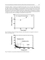
Fig. 3. An example of transmission power control
Fig.3 shows an example of the above transmission power control, which means that the
tra-nsmission power of each sensor node is switched to low power according to the above
con-dition. In this example, node (m) is a load concentration node. Node (m) has
autonomously transmitted the data packet to node (r) with the greatest connective value
within low power range by low power because its own residual energy has become less
than the set threshold [T

e
]. By switching to low power, the energy consumption of node
(m) is saved, but node (k) and node (l) may continue to transmit the data packet to node
(m) because they cannot grasp the updated connective value of node (m). In our scheme,
therefore, every tenth data packet from the node switched to low power is transmitted by
high power.
3. Simulation experiment
Through simulation experiments on a wireless sensor network with multiple sinks, the perf-
ormances of our scheme have been investigated in detail to verify its effectiveness.
3.1 Conditions of simulation
In a large scale and dense wireless sensor network with multiple sinks consisting of many
static sensor nodes placed in a large scale observation area, only sensor nodes that
Autonomous Decentralized Control Scheme for Long-Term
Operation of Large Scale and Dense Wireless Sensor Networks with Multiple Sinks

451
detected abnormal data set were assumed to transmit the measurement data. The
conditions of the si-mulation which were used in the experiments performed are shown in
Table1. In the initial state of the simulation experiments, static sensor nodes are randomly
arranged in the set ex-perimental area, and multiple sinks are placed on the boundaries
containing the corners of this area. The network configuration is shown in Fig.4. In the
experiments performed, the value attenuation factor accompanying hop (dr) and the
“value to self” of each sink node in-troduced in our scheme were set to 0.5 and 100.0,
respectively.

2 or 3Number of sinks
6 [bytes]Size of each control packet
18 [bytes]Size of each data packet
0.2 [J] or 0.5[J]Battery capacity of each sensor node
150m or 200mRange of radio wave

750, 1000, 1250Number of sensor nodes
2400m × 2400mSimulation size
2 or 3Number of sinks
6 [bytes]Size of each control packet
18 [bytes]Size of each data packet
0.2 [J] or 0.5[J]Battery capacity of each sensor node
150m or 200mRange of radio wave
750, 1000, 1250Number of sensor nodes
2400m × 2400mSimulation size

Table 1. Conditions of simulation

evaluation node

Fig. 4. Large scale and dense wireless sensor network consisting of many static sensor
nodes
In the experimental results reported, our scheme (Matsumoto et al., 2010) is evaluated thro-
ugh a comparison with existing ones (Dubois-Ferriere et al., 2004; Oyman & Ersoy, 2004;
Ohtaki et al., 2006; Utani et al., 2008) where the parameter settings that produced good
results in a preliminary investigation were adopted in preference to existing ones.
3.2 Experimental results on simulation model with two sinks
In this subsection, experimental results on the simulation model with two sinks of our sche-
me without transmission power control are shown, where the number of sensor nodes was
1000, the range of radio wave and the battery capacity of each sensor node were set to 150m
and 0.5J, respectively.

Environmental Monitoring

452

evaluation nodeevaluation nodeevaluation node

evaluation nodeevaluation nodeevaluation node

(a) 1 to 500 data packets (b) 1 to 1000 data packets

evaluation nodeevaluation nodeevaluation node

evaluation nodeevaluation nodeevaluation node

(c) 1 to 2000 data packets (d) 1 to 3000 data packets

Fig. 5. Routes used by applying our scheme to the simulation model with two sinks
As the first experiment on the simulation model with two sinks, it was assumed that the ev-
aluation node marked in Fig.4 detected an abnormal value and transmitted the data packet
with this abnormal value periodically. The routes used by applying our scheme are shown
in Fig.5. Of the 3000 data packets transmitted from the evaluation node, the routes used by
the first 500 data packets are illustrated in Fig.5(a), those used by the 1000 data packets are
in Fig.5(b), those used by the 2000 data packets are in Fig.5(c), and those used by a total of
3000 data packets are in Fig.5(d). From Fig.5, it can be confirmed that our scheme enables
the autonomous load-balancing transmission of data packets to two sinks using multiple ro-
utes.
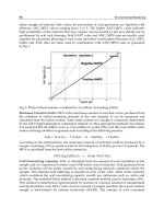
Next, it was assumed that data packets were periodically transmitted from a total of 20
sens-or nodes placed in the set simulation area. In Fig.6, the transition of the delivery ratio
of the total number of data packets transmitted from a total of 20 randomly selected
Autonomous Decentralized Control Scheme for Long-Term
Operation of Large Scale and Dense Wireless Sensor Networks with Multiple Sinks

453
sensor nodes is shown, and the lifetime of the simulation model with two sinks, as in

Fig.5, is compared. In Fig.6, the existing schemes in Ohtaki et al., 2006 and Utani et al.,
2008, which belong to the category of ant-based routing algorithms, are denoted as MUAA
and AAR, respectively. The existing scheme in Dubois-Ferriere et al., 2004 and Oyman and
Ersoy, 2004, which describe representative data gathering for a wireless sensor network
with multiple sinks, is denoted as NS. From Fig.6, it can be confirmed that our scheme
denoted as Proposal in Fig.6 achieves a longer-term operation of a wireless sensor network
with multiple sinks than the existing ones because it improves and balances the load of
each sensor node by the communication load reduction for network control and the
autonomous load-balancing data transmission. Through simulation experiments, it was
verified that our scheme (Matsumoto et al., 2010) is substantially advantageous for the
long-term operation of a large scale and dense wireless sensor network with multiple
sinks.

0%
20%
40%
60%
80%
100%
0 1000 2000 3000 4000 5000 6000 7000 8000
The total transmission number of data packets
Delivery ratio (%)
MUAA
AAR
NS
Proposal

Fig. 6. Transition of delivery ratio
3.3 Experimental results on simulation model with three sinks
In this subsection, through experimental results on the simulation model with three

sinks, the effectiveness of the transmission power control introduced in our scheme is
evaluated. In the following experimental results, the battery capacity of each sensor node
was set to 0.2J, and the range of radio wave of high power transmission in each sensor
node was set to 200 m and it of low power transmission in each sensor node was set to
150m.
As the first experiment on the simulation model with three sinks, it was assumed that the
evaluation node marked in Fig.4 detected an abnormal value and transmitted the data pack-
et with this abnormal value periodically, as in the above subsection 3.2. The routes used by

Environmental Monitoring

454
applying our scheme are shown in Figs.7, 8 and 9, where the number of sensor nodes is
1000. In Figs.7, 8 and 9, T
e
was set to 0.0J, E×0.5J, and E×0.9J, where E indicates the battery
capaci-ty of each sensor node. Of the 3000 data packets transmitted from the evaluation
node, the r-outes used by the first 500 data packets are illustrated in Figs.7, 8 and 9(a), those
used by the 1000 data packets are in Figs.7, 8 and 9(b), those used by the 2000 data packets
are in Figs.7, 8 and 9(c), and those used by a total of 3000 data packets are in Figs.7, 8 and
9(d). From Figs. 7, 8 and 9, it can be confirmed that the effect of our scheme is extended by
early switching to low power.


evaluation nodeevaluation node

evaluation nodeevaluation node

(a) 1 to 500 data packets (b) 1 to 1000 data packets

evaluation nodeevaluation node

evaluation nodeevaluation node

(c) 1 to 2000 data packets (d) 1 to 3000 data packets

Fig. 7. Routes used by applying our scheme (T
e
= 0.0J )
Next, it was assumed that data packets were periodically transmitted from a total of 20 sens-
or nodes placed in the set simulation area. In Figs.10, 11 and 12, the transition of the delivery
ratio of the total number of data packets transmitted from a total of 20 randomly selected se-
Autonomous Decentralized Control Scheme for Long-Term
Operation of Large Scale and Dense Wireless Sensor Networks with Multiple Sinks

455
nsor nodes is shown, and the lifetime of the simulation model with three sinks, as in Figs.7,
8 and 9, is compared. From Figs.10, 11 and 12, it can be confirmed that the effect of our sche-
me is extended by early switching to low power in high node density.


evaluation nodeevaluation node

evaluation nodeevaluation node

(a) 1 to 500 data packets (b) 1 to 1000 data packets

evaluation nodeevaluation node

evaluation nodeevaluation node

(c) 1 to 2000 data packets (d) 1 to 3000 data packets

Fig. 8. Routes used by applying our scheme (T
e
= E×0.5J )
3.4 Discussion
To facilitate ubiquitous information environments by wireless sensor networks, their
control mechanisms should be adapted to the variety of types of communication,
depending on ap-plication requirements and the context. Currently, adaptive
communication protocols for the long-term operation of the above ubiquitous sensor
networks (Intanagonwiwat et al., 20-03; Silva et al., 2004; Heidemann et al., 2003;
Krishnamachari & Heidemann, 2003; Wakabay-ashi et al., 2007) are under study. In

Environmental Monitoring

456
addition, the advanced design schemes of wireless sens-or networks, such as sink node
allocation schemes based on the particle swarm optimization algorithms aiming to
minimize total hop counts in a network and to reduce the energy cons-umption of each
sensor node (Kumamoto et al., 2008; Yoshimura et al., 2009; Taguchi et al., 2010), and
forwarding node set selection schemes (Nagashima et al., 2009; Sasaki et al., 2010) and
forwarding power adjustment scheme (Nagashima et al., 2011) for adaptive and efficie-nt
query dissemination throughout a wireless sensor network, are positively researched.
By coupling our scheme (Matsumoto et al., 2010) with the above advanced design
schemes, it can be expected that the lifetime of a wireless sensor network is moreover
prolonged.


evaluation nodeevaluation node

evaluation nodeevaluation node

(a) 1 to 500 data packets (b) 1 to 1000 data packets

evaluation nodeevaluation node

evaluation nodeevaluation node

(c) 1 to 2000 data packets (d) 1 to 3000 data packets

Fig. 9. Routes used by applying our scheme (T
e
= E×0.9J )
Autonomous Decentralized Control Scheme for Long-Term
Operation of Large Scale and Dense Wireless Sensor Networks with Multiple Sinks

457

0%
20%
40%
60%
80%
100%
120%
0 1000 2000 3000 4000 5000 6000 7000
The total transmission number of data packets
Delivery ratio (%)
N

S
P
roposal (Te=
0.0J
)
P
roposal (Te=E
×0.5J
)
P
roposal (Te=E
×0.9J
)
100% line
(
NS
)
100% line
(
P
ro
p
osal
)


Fig. 10. Transition of delivery ratio (The number of sensor nodes is 750 )


0%

20%
40%
60%
80%
100%
120%
0 1000 2000 3000 4000 5000 6000 7000
The total transmission number of data packets
Delivery ratio (%)
N
S
P
roposal (Te=
0.0J
)
P
roposal
(
Te=E
×0.5J
)
P
roposal (Te=E
×0.9J
)
100% line
(
NS
)
100% line

(
P
ro
p
osal
)


Fig. 11. Transition of delivery ratio (The number of sensor nodes is 1000 )

Environmental Monitoring

458

0%
20%
40%
60%
80%
100%
120%
0 1000 2000 3000 4000 5000 6000 7000
The total transmission number of data packets
Delivery ratio (%)
N
S
P
roposal (Te=
0.0J
)

P
roposal (Te=E
×0.5J
)
P
roposal (Te=E
×0.9J
)
100% line
(
NS
)
100% line
(
P
ro
p
osal
)

Fig. 12. Transition of delivery ratio (The number of sensor nodes is 1250 )
4. Conclusions
In this chapter, a new data gathering scheme with transmission power control that adaptive-
ly reduces the load of load-concentrated nodes and facilitates the long-term operation of a
large scale and dense wireless sensor network with multiple sinks, which is an autonomous
load-balancing data transmission one devised by considering the application environment
of a wireless sensor network to be a typical example of complex systems, has been represen-
ted. In simulation experiments, the performances of this scheme were compared with those
of the existing ones. The experimental results indicate that this scheme is superior to the exi-
sting ones and has the development potential as a promising one from the viewpoint of the

long-term operation of wireless sensor networks. Future work includes a detailed evaluation
of the parameters introduced in this scheme in various network environments.
5. Acknowledgment
The development of a new autonomous decentralized control scheme for the long-term ope-
ration of wireless sensor networks with multiple sinks represented in this chapter is suppor-
ted by the Grant-in-Aid for Scientific Research (Grant No.21500082) from the Japan Society
for the Promotion of Science.
6. References
Akyildiz, I.; Su, W.; Sankarasubramaniam, Y. & Cayirci, E. (2002). Wireless sensor networks:
A survey, Computer Networks Journal, Vol.38, No.4, 393-422
Autonomous Decentralized Control Scheme for Long-Term
Operation of Large Scale and Dense Wireless Sensor Networks with Multiple Sinks

459
Clausen, T. & Jaquet, P. (2003). Optimized link state routing protocol, Request for Comments
(RFC) 3626
Dasgupta, K.; Kalpakis, K. & Namjoshi, P. (2003). An efficient clustering-based heuristic for
data gathering and aggregation in sensor networks, Proceedings of IEEE Wireless Co-
mmunications and Networking Conference, 16-20
Dubois-Ferriere, H.; Estrin, D. & Stathopoulos, T. (2004). Efficient and practical query scop-
ing in sensor networks, Proceedings of IEEE International Conference on Mobile Ad-Hoc
and Sensor Systems, 564-566
Heidemann, J.; Silva, F. & Estrin, D. (2003). Matching data dissemination algorithms to appl-
ication requirements, Proceedings of 1st ACM Conference on Embedded Networked Sens-
or Systems, 218-229
Heinzelman, W.R.; Chandrakasan, A. & Balakrishnan, H. (2000). Energy-efficient communi-
cation protocol for wireless microsensor networks, Proceedings of Hawaii Internation-
al Conference on System Sciences, 3005-3014
Intanagonwiwat, C.; Govindan, R.; Estrin, D.; Heidemann, J. & Silva, F. (2003). Directed diff-
usion for wireless sensor networking, ACM/IEEE Transactions on Networking, Vol.11,

2-16
Jin, Y.; Jo, J. & Kim, Y. (2008). Energy-efficient multi-hop communication scheme in cluster-
ed sensor networks, International Journal of Innovative Computing, Information and Co-
ntrol, Vol.4, No.7, 1741-1749
Johnson, D.B.; Maltz, D.A.; Hu, Y.C. & Jetcheva, J.G.(2003). The dynamic source routing pro-
tocol for mobile ad hoc networks, IETF Internet Draft, draft-ietf-manet-dsr-09.txt
Krishnamachari, B. & Heidemann, J. (2003). Application-specific modeling of information r-
outing in wireless sensor networks, Technical Report, ISI-TR-2003-576, USC-ISI
Kumamoto, A.; Utani, A. & Yamamoto, H. (2008). Improved particle swarm optimization for
locating relay-dedicated nodes in wireless sensor networks, Proceedings of 2008 Joint
4th International Conference on Soft Computing and Intelligent Systems and 9th Internati-
onal Symposium on Advanced Intelligent Systems, 1971-1976
Matsumoto, K.; Utani, A. & Yamamoto, H. (2009). Adaptive and efficient routing algorithm
for mobile ad-hoc sensor networks, ICIC Express Letters, Vol.3, No.3(B), 825-832
Matsumoto, K.; Utani, A. & Yamamoto, H. (2010). Bio-inspired data transmission scheme to
multiple sinks for the long-term operation of wireless sensor networks, International
Journal of Artificial Life and Robotics, Vol.15, No.2, 189-194
Nagashima, J.; Utani, A. & Yamamoto, H. (2009). Efficient flooding method using discrete p-
article swarm optimization for long-term operation of sensor networks, ICIC Expre-
ss Letters, Vol.3, No.3(B), 833-840
Nagashima, J.; Utani, A. & Yamamoto, H. (2011). A study on efficient query dissemination
in distributed sensor networks -Forwarding power adjustment of each sensor node
using particle swarm optimization-, Proceedings of 16th International Symposium on
Artificial Life and Robotics, 703-706
Nakano, H.; Utani, A.; Miyauchi, A. & Yamamoto, H. (2009). Data gathering scheme using c-
haotic pulse-coupled neural networks for wireless sensor networks, IEICE Transact-
ions on Fundamentals
, Vol.E92-A, No.2, 459-466
Nakano, H.; Utani, A.; Miyauchi, A. & Yamamoto, H. (2011). Chaos synchronization-based
data transmission scheme in multiple sink wireless sensor networks, International J-

ournal of Innovative Computing, Information and Control, Vol.7, No.4, 1983-1994

Environmental Monitoring

460
Ogier, R.; Lewis, M. & Templin, F.(2003). Topology dissemination based on reverse-path for-
warding (TBRPF), IETF Internet Draft, draft-ietf-manet-tbrpf-10.txt
Ohtaki, Y.; Wakamiya, N.; Murata, M. & Imase, M. (2006). Scalable and efficient ant-based
routing algorithm for ad-hoc networks, IEICE Transactions on Communications, Vol.E
89-B, No.4, 1231-1238
Oyman, E.I. & Ersoy, C. (2004). Multiple sink network design problem in large scale wireless
sensor networks, Proceedings of 2004 International Conference on Communications, Vol.
6, 3663-3667
Perkins, C.E. & Royer, E.M. (1999). Ad hoc on-demand distance vector routing, Proceedings of
2nd IEEE Workshop on Mobile Computing Systems and Applications, 90-100
Rajagopalan, R. & Varshney, P.K. (2006). Data aggregation techniques in sensor networks: A
survey, IEEE Communications Surveys and Tutorials, Vol.8, 48-63
Sasaki, T.; Nakano, H.; Utani, A.; Miyauchi, A. & Yamamoto, H. (2010). An adaptive selecti-
on scheme of forwarding nodes in wireless sensor networks using a chaotic neural
network, ICIC Express Letters, Vol.4, No.5(A), 1649-1655
Silva, F.; Heidemann, J.; Govindan, R. & Estrin, D. (2004). Directed diffusion, Technical
Report, ISI-TR-2004-586, USC-ISI
Subramanian, D.; Druschel, P. & Chen, J. (1998). Ants and reinforcement learning: A case st-
udy in routing in dynamic networks, Technical Report TR96-259, Rice University
Taguchi, Y.; Nakano, H.; Utani, A.; Miyauchi, A. & Yamamoto, H. (2010). A competitive par-
ticle swarm optimization for finding plural acceptable solutions, ICIC Express Lette-
rs, Vol.4, No.5(B), 1899-1904
Utani, A.; Orito, E.; Kumamoto, A. & Yamamoto, H. (2008). An advanced ant-based routing
algorithm for large-scale mobile ad-hoc sensor networks, Transactions on SICE, Vol.
44, No.4, 351-360

Wakabayashi, M.; Tada, H.; Wakamiya, N.; Murata, M. & Imase, M. (2007). Proposal and ev-
aluation of a bio-inspired adaptive communication protocol for sensor networks, I-
EICE Technical Report, Vol.107, No.294, 89-94
Wakamiya, N. & Murata, M.(2005). Synchronization-based data gathering scheme for sensor
networks, IEICE Transactions on Communications, Vol.E88-B, No.3, 873-881
Xia, L.; Chen, X. & Guan, X.(2004). A new gradient-based routing protocol in wireless sensor
networks, Lecture Notes in Computer Science, Vol.3605, 318-325
Yamamoto, I.; Ogasawara, K.; Ohta, T. & Kakuda, Y. (2009). A hierarchical multicast routing
using inter-cluster group mesh structure for mobile ad hoc networks, IEICE Transa-
ctions on Communications, Vol.E92-B, No.1, 114-125
Yoshimura, M.; Nakano, H.; Utani, A.; Miyauchi, A. & Yamamoto, H. (2009). An effective al-
location scheme for sink nodes in wireless sensor networks using suppression PSO,
ICIC Express Letters, Vol.3, No.3(A), 519-524
0
Collaborative Environmental Monitoring with
Hierarchical Wireless Sensor Networks
Qing Ling
1
,GangWu
1
and Zhi Tian
2
1
Department of Automation, University of Science and Technology of China
2
Department of Electrical and Computer Engineering, Michigan Technological University
1
China
2
USA

1. Introduction
In the last decade, advances in wireless communication and micro-fabrication have motivated
the development of large-scale wireless sensor networks (Akyildiz et al., 2002; Yick et al.,
2008). A large number of low-cost sensor nodes, equipped with sensing, computing, and
communication units, organize themselves into a multi-hop network. The wireless sensor
network takes measurements from the environment, processes the sensory data, and transmits
the sensory data to end-users. Beginning from the seminar work in (Estrin et al., 1999; 2002),
the wireless sensor network technology has been well recognized as a revolutionary one that
transforms everyday life. Typical applications of wireless sensor networks include military
target tracking and surveillance (Simon et al., 2004; He et al., 2006), precise agriculture
(Langendoen et al., 2006; Wark et al., 2007), industrial automation (Gungor and Hancke,
2009), structural health monitoring (Li and Liu, 2007; Ling et al., 2009), environmental and
habitat monitoring (Zhang et al., 2004; Corke et al., 2010), to name a few.
1.1 Network infrastructure
To organize the large amount of sensor nodes and enable efficient data collection, a wireless
sensor network generally adopts one of the following three infrastructures: centralized,
decentralized, and hierarchical. In the centralized infrastructure, sensor nodes transmit
the sensory data to the fusion center via multi-hop communication. In the decentralized
infrastructure, each sensor node firstly refines the sensory data through collaborative and
decentralized in-network processing with the neighboring sensor nodes, and secondly
transmits the refined data to the fusion center. While in the hierarchical infrastructure, sensor
nodes are divided into multiple clusters, and sensor nodes within one cluster send their
sensory data to the cluster head. These cluster heads either transmit the collected sensory data
to the fusion center, or collaboratively process them and transmit the refined one to the fusion
center. These two different implementations of the hierarchical infrastructure, centralized
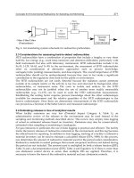
processing and decentralized collaboration, are depicted in Figure 1.
In deploying a wireless sensor network, the choice of its infrastructure is decided by
several key factors: energy, bandwidth, robustness, etc. Sensor nodes are often equipped
with batteries and recharging is difficult. Since wireless data transmission is the main
source of energy consumption of a sensor node (Sadler, 2005), the network infrastructure

26
2 Will-be-set-by-IN-TECH


Fusion Center
Cluster Heads
Sensor Nodes


Cluster Heads
Sensor Nodes
Fig. 1. Two different schemes of implementing the hierarchical infrastructure: (TOP)
centralized processing in a fusion center and (BOTTOM) decentralized collaboration among
cluster heads.
should guarantee that each sensor node has low data transmission rate while successfully
accomplishing the data collection task. Bandwidth is also a kind of precious resource in
wireless environment; over-competition of wireless channels leads to frequent retransmission
and hence consumes more energy. Further, sensor nodes are often fragile due to being out of
batteries or other physical damages. The network infrastructure should be carefully designed
such that the failure of few sensor nodes shall not result in the malfunction of the whole
network.
When the network size is small, the centralized infrastructure is an acceptable choice. Take
a volcano monitoring network containing 3 sensor nodes (Werner-Allen et al., 2005) as an
example, these sensor nodes directly connect to a fusion center which collects sensory data
and transmits them to the end-user. Later on the network is extended to the scale of 16
sensor nodes (Werner-Allen et al., 2006), and the sensor nodes communicate with the fusion
center via multi-hop relays. However, for GreenOrbs (Liu et al., 2011), a large-scale forest
monitoring network composed of up to 330 sensor nodes, experiments demonstrate that
sensor nodes within some "hot areas" may face higher competition for bandwidth, consume
more energy, and be more sensitive to the failure of sensor nodes. The decentralized

infrastructure, on the other hand, has great potential to reduce the total amount of transmitted
data and hence improve the energy efficiency via in-network collaboration; further, it also
enhances robustness of the network since all sensor nodes play equal roles (Ling and Tian,
2010). Nevertheless, collaboration of the sensor nodes brings more difficulty to network
coordination, and is subject to the limited processing and communication capabilities of
sensor nodes. For this reason, the decentralized infrastructure is still far from practical
applications. To the best of our knowledge, most large-scale wireless sensor networks are
deployed with the hierarchical infrastructure. Following we give some examples: ExScal,
an intrusion detection network with more than 1000 sensor nodes and more than 200
backbone nodes (Arora et al., 2005); VigilNet, a military surveillance network with 200 sensor
nodes (He et al., 2006); Trio, a target tracking network with 557 solar-powered sensor nodes
462
Environmental Monitoring
Collaborative Environmental Monitoring with Hierarchical Wireless Sensor Networks 3
(Dutta et al., 2006); SenseScope, an environmental monitoring network consisting of from 3 to
97 sensor nodes (Barenetxea et al., 2008). In view of this fact, we will focus on the design of a
hierarchical wireless sensor network.
1.2 Our contributions
In some hierarchical wireless sensor networks such as ExScal (Arora et al., 2005), the cluster
heads are specifically designed, having better data processing and wireless communication
abilities than general sensor nodes, and equipped with stronger or even uninterruptible power
sources. These cluster heads can directly transmit the collected data to a remote fusion center,
without introducing any collaborative processing among cluster heads. However, in most
wireless sensor networks, cluster heads are elected from sensor nodes to simplify design,
deployment, and maintenance. For example, in the LEACH protocol (Heinzelman et al.,
2002), sensor nodes autonomously elect cluster heads, aiming at evenly distributing energy
consumption among all sensor nodes so that there are no overly-utilized sensor nodes that
will run out of energy before the others. In this case, how to process the collected sensory
data in the cluster heads is a critical problem to accomplishing the data collection task while
maximizing the network lifetime.

This chapter addresses this problem; specifically, we study a generalized environmental
monitoring model with large-scale hierarchical wireless sensor networks, and focus on two
questions: for cluster heads in a hierarchical network, should they collaborate or not collaborate
and how can they collaborate. Our contributions are two-fold.
First, through theoretical analysis and simulation validation, we make the following
recommendations on whether to collaborate or not: when each cluster head has a large
amount of data to process (namely, each cluster contains a large number of sensor nodes)
and multi-hop relay is necessary to communicate with a fusion center (namely, cluster heads
have limited communication range), decentralized data processing among cluster heads is
more efficient; otherwise centralized decision-making with the aid of a fusion center can be
advantageous.
Previous work, such as (Rabbat and Nowak, 2004; Aldosari and Moura, 2004), has suggested
similar network design principles in the context of decentralized infrastructures: when
each sensor node collects a large amount of data or the size of the network is large,
collaborative processing is more efficient than centralized decision-making. This paper
extends the conclusions to hierarchical networks, and compares decentralized versus
centralized processing among cluster heads rather than among all sensor nodes.
Second, we develop a decentralized collaborative algorithm for decision making among the
sub-network of cluster heads, after they have collected sensory data from local sensor nodes
within their individual clusters. Particularly, we study a typical environment monitoring
application, in which a large-scale hierarchical wireless sensor network is deployed to
monitor sparsely occurring phenomena over a large sensing field. The monitoring problem
is formulated as a non-negative quadratic program, which optimizes a sparse decision vector
depicting the spatial map of the phenomena of interest. An optimal iterative algorithm, in
which cluster heads iteratively exchange information and make decisions, is proposed based
on the alternating direction method of multipliers (ADMM) (Bertsekas and Tsitsiklis, 1997).
Our development is permeated with the benefits of compressive sensing (Donoho et al., 2006).
Exploiting the sparse nature of the unknown phenomena, we allow the number of sensor
nodes to be much smaller than what would have been required in a traditional scheme for
463

Collaborative Environmental Monitoring with Hierarchical Wireless Sensor Networks
4 Will-be-set-by-IN-TECH
sensing at high spatial resolution over a large field. In this sense, our proposed algorithm is
also applicable to other compressive sensing problems in distributed systems.
1.3 Chapter organization
The rest of this chapter is organized as follows. We first give a brief survey on the applications
of wireless sensor networks in environmental monitoring. Second, we study a generalized
environmental monitoring model with large-scale hierarchical wireless sensor networks and
develop a decentralized collaborative algorithm for decision making among the cluster heads.
Finally we discuss the design consideration, namely, to collaborate or not to collaborate, based
on theoretical analysis and simulation results.
2. A brief survey
In this section, we give a brief survey on the applications of wireless sensor networks in
environmental and habitat monitoring. Though this overview is far from complete, it reflects
the promising future of the wireless sensor network technology in helping us understand and
protect natural environment.
For environmental and habitat monitoring applications, one of the first known practical
wireless sensor networks was deployed by a group at Berkeley in 2002, on Great Duck Island
on the coast of Maine, USA. Two networks with a total of 147 sensor nodes collect data to study
the ecology of the Leach’s Storm Petrel (Szewsczyk et al., 2004). Later on, the Macroscope
system which contains 33 sensor nodes, also developed at Berkeley, was used for microclimate
monitoring of a redwood tree (Tolle et al., 2005). Another notable application is ZebraNet,
which used GPS technology to record position data in order to track long term animal
migrations. In the prototype system, researchers deployed 7 sensor nodes on zebras in Kenya
(Zhang et al., 2004). Energy harvesting technologies have also attracted much research interest
to address the challenge of energy supply in remote environmental monitoring applications.
One successful example is LUSTER, which was developed at University of Virginia, featuring
a specifically designed hybrid multichannel energy harvesting device (Selavo et al., 2007).
Accompanied with the unprecedented data collection opportunities, data processing also
emerges as a new challenge in the wireless sensor network technology. The data processing

task is indeed application-oriented. For example, an ellipsoids-based anomaly detection
algorithm was designed to monitor unusual and anomalous behaviors in a particular marine
ecosystem (Bedzek et al., 2011). The network was deployed in 2009 at the Heron Island,
Australia, as part of the Great Barrier Reef Ocean Observation System.
One significant advantage of wireless sensor networks over traditional data collection
techniques is that they can be applied in harsh environments. For example, in the GlacsWeb
system, researchers at University of Southampton deployed 9 sensor nodes inside a glacier
(Martinez et al., 2004). The sensor nodes monitored pressure, temperature, and tilt, in
order to monitor subglacial bed deformation. Even on active volcanos, which are often
forbidden areas for data collection, wireless sensor networks can still work well. In the
work of (Werner-Allen et al., 2005; 2006), one small sensor network with 3 sensor nodes was
deployed on Vlcan Tungurahua in Ecuador as a proof of concept in 2004; then in 2005, the
network size was extended to 16 sensor nodes. Wireless sensor networks are also fit for
aquatic environmental monitoring applications. In (Alippi et al., 2011), a robust, adaptive,
and solar-powered network was developed in 2007 for such an application. The network
was deployed in Queensland, Australia, for monitoring the underwater luminosity and
temperature, information necessary to derive the health status of the coralline barrier. At
464
Environmental Monitoring
Collaborative Environmental Monitoring with Hierarchical Wireless Sensor Networks 5
the same time, sensory data can be used to provide quantitative indications related to cyclone
formations in tropical areas.
However, applying wireless sensor networks in environmental monitoring is still a
challenging task when the network size is large. When the number of sensor nodes increases,
difficulties emerge for system integration (creating an end-to-end system that delivers data
to the end-user), performance (reliability, accuracy, and calibration), productivity (how well
the sensory data assists the end-user and how to reduce the total cost in implementing
the wireless sensor network), etc (Corke et al., 2010). One negative example is reported in
(Langendoen et al., 2006), in which researchers at Delft University of Technology deployed
a large-scale network in a potato field to improve the protection of potatoes against disease.

The application was not successful due to unanticipated issues; nevertheless, the lessons are
precious, such as software, hardware, and even team coordination. A systematic discussion,
named as ”the hitchhiker’s guide”, is provided in (Barenetxea et al., 2008). Based on the
deployment of a wireless sensor network on a rock glacier located at a mountain in the
Swiss Alps, this guide covers almost all stages of a project, from hardware and software
development, testing and preparation, to deployment. One of the recent efforts to investigate
the practical implementations of large-scale wireless sensor networks is the GreenOrbs system
(Liu et al., 2011). The network with 330 sensor nodes was deployed in Tianmu Mountian,
China, aiming at all-year-around ecological surveillance in the forest. It is shown that many
traditional design guidelines for small-scale wireless sensor networks can be questionable for
large-scale applications.
3. Problem formulation
In this chapter, we focus on a generalized event detection model for environmental monitoring
applications. Let us consider a large-scale wireless sensor network randomly deployed in a
two-dimensional area for monitoring sparsely occurring events. The network has a set of L
sensor nodes, denoted as
L = {v
l
}
L
l
=1
. Sensor nodes are divided into I clusters, each having
one cluster head in the set
I = {c
i
}
I
i
=1

. Sensor nodes within a cluster are able to directly
transmit measurements to the cluster head, and the cluster head is aware of the positions of
all sensor nodes within its cluster. Further, the cluster heads have a common communication
range r
C
such that the sub-network of cluster heads is bi-directionally connected.
3.1 Basic assumptions
Suppose that at each sampling time, multiple phenomena may occur in the sensing field. Our
objective is to detect and identify the source locations and estimate their amplitudes from
sensory measurements. We make the following basic assumptions for the sensing problem of
interest, similar to those in (Bazerque and Giannakis, 2010):
(A1): The sensing field is viewed through a spatial grid with K grid points denoted by
K =
{
g
k
}
K
k
=1
, whose locations are known to the corresponding cluster heads. Each event can occur
only at a grid point, indicating the spatial resolution offered by this sensor network. The
amplitude of an event occurring at grid point g
k
is x
k
.
(A2): The influence of a unit-amplitude event at grid point g
k
on a sensor point v

l
is f
kl
.
Generally speaking, f
kl
is decided by the distance d
kl
between g
k
and v
l
.
(A3): The measurement of one sensor node is the linear superposition of the influences of
all phenomena plus random noise. Mathematically, the measurement b
l
of sensor node v
l
is hence b
l
=
∑
K
k=1
f
kl
x
k
+ e
l

in which x
k
is the amplitude of event at g
k
∈Kand e
l
is
measurement noise.
465
Collaborative Environmental Monitoring with Hierarchical Wireless Sensor Networks
6 Will-be-set-by-IN-TECH
Fig. 2. The sensor nodes denoted as solid squares are uniformly randomly deployed in the
monitoring area. The candidate positions for phenomena are grid points denoted as solid
dots. Phenomena denoted as pentagrams occur at the current snapshot, and the shadow
regions illustrate the influence of phenomena.
These assumptions are depicted in Figure 2. The sensor nodes denoted as solid squares
are uniformly randomly deployed in the monitoring area. The candidate positions for
phenomena are grid points denoted as solid dots. Phenomena denoted as pentagrams occur
at the current snapshot, and the shadow regions illustrate the influence of phenomena.
The assumption (A1) simplifies the recovery problem by confining the sources of phenomena
to grid points. Without this assumption, an alternative way is to use positions and amplitudes
of the sources as decision variables and formulate a least squares problem. However, this
formulation is highly nonlinear and intractable, since the number of decision variables is even
unknown. Based on (A1), we can formulate the otherwise nonlinear problem as recovering
the vector x
=[x
1
, , x
K
]

T
from linear measurements b
l
, ∀l.Entriesinx with nonzero values
reveal the locations and amplitudes of the multiple phenomena of interest. This assumption
approximately holds when the grid points are dense; namely, the density of the grid points
decides the spatial resolution of the recovery algorithm.
The assumption (A2) describes the influence of one event on the entire sensing field. For
example, in target tracking or nuclear radioactive detection, the influence of a source decreases
polynomially as the distance increases. Without loss of generality, we define the influence
function as f
kl
= exp(−d
2
kl
/σ
2
) for grid point g
k
and sensor point v
l
,whereσ is a common
constant. This Gaussian-shaped function well approximates the influence of many practical
events.
Based on the assumption (A3), we readily have the following least squares formulation for
recovering x:
min
∑
v
l

∈L
(b
l
−
∑
K
k
=1
f
kl
x
k
)
2
,
(1)
or equivalently in a matrix form:
min
||Fx −b||
2
2
.
(2)
Here b
=[b
1
, , b
L
]
T

is the measurement vector and F is the L × K influence matrix with its
l-th row given by
[ f
1l
, , f
Kl
].
466
Environmental Monitoring
Collaborative Environmental Monitoring with Hierarchical Wireless Sensor Networks 7
Nevertheless, the least squares formulation (2) ignores the sparsity of the vector x.Noticethat
when the grid is dense, the number of events is generally much smaller than the number of
grid points; hence the vector x is a sparse vector with a large amount of zero entries. Without
considering this prior knowledge, the least squares formulation (2) leads to a non-sparse
solution, which means a non-neglectable number of false alarms. The sparsity of a signal
vector can be measured by its

1
norm (Donoho et al., 2006). Exploiting the sparse nature of
x to alleviate false alarms, we formulate the following

1
regularized least squares problem
(Kim et al., 2007):
min
λ
2
||Fx −b||
2
2

+ ||x||
1
.
(3)
Here λ is a non-negative weight.
3.2 Decentralized optimization
In a centralized setting, the 
1
regularized least squares problem (3) has been extensively
studied in both signal processing and numerical optimization communities (Donoho et al.,
2006; Figueiredo et al., 2007). However, in a large-scale wireless sensor network, centralized
processing is not efficient in terms of energy consumption and communication overhead. In
contrast, collaborative signal processing among cluster heads is preferred, leading to a robust
and scalable network.
We address this issue by developing a collaborative sparse signal recovery algorithm in the
chapter. Sensor nodes or cluster heads do not necessarily exchange information with a fusion
center; rather, sensor nodes only need to transmit measurements to their cluster heads, and
cluster heads iteratively optimize the decision vector x via exchanging information with their
neighboring cluster heads.
For each cluster head c
i
, let us collect the local measurements {v
l
} within this cluster and their
corresponding l-th rows in the measurement matrix F into a sub-vector b
i
and a sub-matrix F
i
,
for all sensor nodes v

l
whose cluster head is c
i
. Per assumptions (A1) and (A2),eachcluster
head knows all sensor node locations and grid point locations within its cluster, which means
that F
i
is known to c
i
. Hence the problem boils down to the following one: suppose that the local
measurement vector b
i
and corresponding measurement matrix F
i
are available to e ach cluster head c
i
,
∀i, how can we design a decentralized algorithm to recover the signal x via collaboration among the
cluster heads?
Let x
i
denote the local copy of the decision vector x at c
i
, ∀c
i
∈I. Meanwhile, given
the communication range r
C
, the set of neighboring cluster heads of c
i

is denoted by N
i
,
with cardinality
|N
i
|. The formulation in (3) can be transformed to the following consensus
optimization problem:
min
∑
I
i
=1
(
λ
2
||F
i
x
i
−b
i
||
2
2
+
1
I
1
T

x
i
),
s.t. x
i
= x
j
, ∀c
i
∈I, c
j
∈N
i
.
(4)
The K
× 1 all-one vector [1, 1, , 1]
T
is denoted as 1. Here, cluster heads optimize their
own local copies of x separately, and these decision vectors are forced to be equal via the
consensus constraints. An alternative formulation is to force x
i
to consent with the average of
its neighboring decisions, as follows:
min
∑
I
i
=1
(

λ
2
||F
i
x
i
−b
i
||
2
2
+
1
I
1
T
x
i
),
s.t. x
i
=
1
|N
i
|
∑
c
j
∈N

i
x
j
, ∀c
i
∈I.
(5)
It has been proved that if the sub-network of the cluster heads is bi-directionally connected,
then (4) and (5) are equivalent to (3) (Zhu et al., 2007). Both (4) and (5) can be solved similarly,
as below.
467
Collaborative Environmental Monitoring with Hierarchical Wireless Sensor Networks
8 Will-be-set-by-IN-TECH
4. Collaborative environmental monitoring algorithm
We now apply an optimal algorithm, the alternating direction method of multipliers (ADMM)
(Bertsekas and Tsitsiklis, 1997), to solve (4).
4.1 Algorithm development
To solve (4) with the ADMM, we first introduce a new block of auxiliary variables. Then (4)
can be rewritten as:
min
{x
i
},{z
ij
}
∑
I
i
=1
(

λ
2
||F
i
x
i
−b
i
||
2
2
+
1
I
1
T
x
i
),
s.t. x
i
= z
ij
, x
j
= z
ij
, ∀c
i
∈I, c

j
∈N
i
.
(6)
Here z
ij
is an auxiliary vector attached to x
i
and x
j
. The augmented Lagrangian function of
(6) is:
L
a

{x
i
}, {z
ij
}, {β
ij
}, {γ
ij
}

=
∑
I
i

=1
(
λ
2
||F
i
x
i
−b
i
||
2
2
+
1
I
1
T
x
i
)
+
∑
I
i
=1
∑
c
j
∈N

i
β
T
ij
(x
i
−z
ij
)+
d
2
∑
I
i
=1
∑
c
j
∈N
i
||x
i
−z
ij
||
2
2
+
∑
I

i
=1
∑
c
j
∈N
i
γ
T
ij
(x
j
−z
ij
)+
d
2
∑
I
i
=1
∑
c
j
∈N
i
||x
j
−z
ij

||
2
2
,
(7)
in which
{β
ij
} and {γ
ij
} are Lagrange multipliers and d is a positive constant. At time t,the
ADMM optimizes the augmented Lagrangian function as follows:
Step 1: Optimizing the local copies
{x
i
}:
{x
i
(t + 1)} = arg min
{x
i
}
L
a

{x
i
}, {z
ij
(t)}, {β

ij
(t)}, {γ
ij
(t)}

.(8)
Notice that the objective function is separable, x
i
(t + 1) can be updated as:
x
i
(t + 1)=arg min
x
i
(
λ
2
||F
i
x
i
−b
i
||
2
2
+
1
I
1

T
x
i
)
+
∑
c
j
∈N
i
β
T
ij
(t)x
i
+
∑
c
j
∈N
i
γ
T
ji
(t)x
i
+
d
2
∑

c
j
∈N
i
||x
i
−z
ij
(t)||
2
2
+
d
2
∑
c
j
∈N
i
||x
i
−z
ji
(t)||
2
2
.
(9)
Step 2: Optimizing the Auxiliary Variable
{z

ij
}:
{z
ij
(t + 1)} = arg min
{z
ij
}
L
a

{x
i
(t + 1)}, {z
ij
}, {β
ij
(t)}, {γ
ij
(t)}

. (10)
Here the objective functions is also separable. Therefore:
z
ij
(t + 1)=arg min
z
ij
−β
T

ij
(t)z
ij
−γ
T
ji
(t)z
ij
+
d
2
||x
i
(t + 1) − z
ij
||
2
2
+
d
2
||x
j
(t + 1) −z
ij
||
2
2
.
(11)

It has an explicit solution:
z
ij
(t + 1)=
1
2

x
i
(t + 1)+x
j
(t + 1)

+
1
2d

β
ij
(t)+γ
ij
(t)

. (12)
Step 3: Updating the Lagrange Multipliers
{β
ij
} and {γ
ij
}:

β
ij
(t + 1)=β
ij
(t)+d

x
i
(t + 1) −z
ij
(t + 1)

,
γ
ij
(t + 1)=γ
ij
(t)+d

x
j
(t + 1) −z
ij
(t + 1)

.
(13)
468
Environmental Monitoring
Collaborative Environmental Monitoring with Hierarchical Wireless Sensor Networks 9

The updating rules of (9), (11), and (13) can be further simplified. Substituting (12) to (13)
yields:
β
ij
(t + 1)=β
ij
(t)+
d
2

x
i
(t + 1) −x
j
(t + 1)

−
1
2
(β
ij
(t)+γ
ij
(t)),
γ
ij
(t + 1)=γ
ij
(t)+
d

2

x
j
(t + 1) −x
i
(t + 1)

−
1
2
(β
ij
(t)+γ
ij
(t)).
(14)
Sinceweoftensetβ
ij
(0)=γ
ij
(0)=0 where 0 denotes a K ×1 all-zero vector [0, 0, , 0]
T
, (14)
implies that β
ij
(t)=−γ
ij
(t)=γ
ji

(t). Then (12) becomes:
z
ij
(t + 1)=
1
2

x
i
(t + 1)+x
j
(t + 1)

. (15)
and (13) becomes
β
ij
(t + 1)=β
ij
(t)+
d
2

x
i
(t + 1) −x
j
(t + 1)

= γ

ji
(t + 1),
γ
ij
(t + 1)=γ
ij
(t)+
d
2

x
j
(t + 1) −x
i
(t + 1)

= β
ji
(t + 1).
(16)
Summarizing the three sides of (16) and define a new Lagrangian multiplier α
i
=
2
|N
i
|
∑
c
j

∈N
i
β
ij
=
2
|N
i
|
∑
c
j
∈N
i
γ
ji
, the updating rule for α
i
is:
α
i
(t + 1)=α
i
(t)+dx
i
(t + 1) −
d
|N
i
|

∑
c
j
∈N
i
x
j
(t + 1). (17)
Substituting (15) to (9), we have the updating rule for x
i
:
x
i
(t + 1)=arg min
x
i
∑
I
i
=1
(
λ
2
||F
i
x
i
−b
i
||

2
2
+
1
I
1
T
x
i
)
+|N
i
|α
T
i
(t)x
i
+ d
∑
c
j
∈N
i
||x
i
−
1
2

x

i
(t)+x
j
(t)

||
2
2
.
(18)
Iteratively solving (18) and updating (17) leads to the optimal solution of (4).
It should be noted that the problem we are discussing is indeed a special case of compressive
sensing (Donoho et al., 2006). When the number of sensor nodes is smaller than the number
of grid points, down-sampling is achieved via exploiting the sparse nature of the signal x.
From this viewpoint, the proposed decentralized sparse signal recovery algorithm is also
applicable to other compressive sensing problems, in which distributed sensor nodes hold
parts of measurement matrices as well as measurement vectors, and collaboratively make
decisions.
4.2 Algorithm outline
The collaborative sparse signal recovery algorithm is summarized as follows. The algorithm
is fully decentralized, requiring only collaboration between neighboring cluster heads.
————————————————————- ————————————————————-
Algorithm: Collaborative environmental monitoring
————————————————————- ————————————————————-
Step 1: Initialization. At each sampling point, each cluster head collects position information
and measurements from sensors within its cluster. Hence cluster head c
i
knows the partial
measurement matrix F
i

and the partial measurement vector b
i
. The number of cluster heads
I, the non-negative constant λ, and the positive constant d are also known.
Step 2: Communication. At iteration t
+ 1, each cluster head c
i
broadcasts to its neighboring
469
Collaborative Environmental Monitoring with Hierarchical Wireless Sensor Networks
10 Will-be-set-by-IN-TECH
cluster heads to acquire intermediate decision vectors x
j
(t) of iteration t, c
j
∈N
i
.
Step 3: Optimization. At iteration t
+ 1, each cluster head c
i
updates its Lagrange multiplier
α
i
(t + 1) and decision vector x
i
(t + 1) according to (17) and (18).
Step 4: Iteration. Repeat Step 2 and Step 3 until convergence.
————————————————————- ————————————————————-
5. Performance analysis

In this section we will briefly discuss the impact of parameter settings on the performance
of the algorithm, as well as the design choice of a hierarchical wireless sensor network. By
performance we are mainly concerning: 1) quality of recovery, which includes the number of
false alarms and the gap between the true and estimated amplitudes; and 2) convergence rate,
which directly decides the communication burden of the cluster heads.
5.1 Parameter settings
The role of the non-negative weight λ in (3) has been extensively discussed in compressive
sensing literature, such as (Donoho et al., 2006; Figueiredo et al., 2007). There is a constant
λ
min
= 1/||F
T
b||
∞
,suchthatifλ ≤ λ
min
the optimal solution is 0.Whenλ goes to infinity,
the optimal solution has the minimum

1
norm among all points that satisfy F
T
(Fx −b = 0),if
these points exist. Hence if b is noise-free and F is a full rank square matrix, then the optimal
solution goes to the true signal. However large λ generally leads to a non-sparse solution
under the existence of measurement noise.
In Step 1 of the collaborative environmental monitoring algorithm, we need to know I,the
number of cluster heads. This procedure requires multi-hop communications if the cluster
heads are not directly connected with each other. However, accurate knowledge of I is not
necessary since it is the product λI that decides the optimal solution.

The proposed algorithm converges for any given positive constant d; however, the value
of d influences the convergence rate, and thus the communication burden. It is possible
to dynamically increase the value of d to infinity to improve the convergence rate during
the iterative optimization process (Bertsekas and Tsitsiklis, 1997). Due to the extra burden of
updating d, we simply choose d as a constant.
One of the most important advantages of the hierarchical infrastructure is its flexibility to
different application scenarios. By setting I
= 1, the infrastructure turns to be centralized;
while with I
= L and sensors being cluster heads, the network is a fully decentralized one.
This flexibility enables the network to adapt to different application scenarios.
5.2 To Collaborate or not to collaborate
Now we revaluate the order of the required communication load in a hierarchical network
without any fusion center. First, at the data acquisition stage, cluster heads need to
collect measurements from sensor nodes and construct the local measurement matrix, at
communication cost on the order
∼ O(L). Second, at the optimization stage, one cluster head
needs to transmit its decision vector to each neighboring cluster head at each iteration. The
lengths of decision vectors are all K; the average number of neighboring cluster heads varies
from
∼ O(1) (multi-hop communications) to ∼ O(I) (one-hop communications) depending
on the communication range r
C
of cluster heads. Denote the number of iterations as T,which
is in general influenced by the choices of d and λ,aswellasthetopologyofthenetwork.
Therefore the overall communication load ranges from O
(KIT) to O(KI
2
T).
470

Environmental Monitoring