Heat and Mass Transfer Modeling and Simulation Part 7 doc

Heat and Mass Transfer in External Boundary Layer Flows Using Nanofluids
111
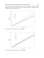
This parameter, drawn in Figures 18 and 19, which is calculated within the thermal
boundary layer, evolves linearly along the wall. Strong differences are observed with the
variation of the particle volume fraction.



Fig. 18. Thermal flow rate for CuO / water nanofluid



Fig. 19. Thermal flow rate for Alumina / water nanofluid

Heat and Mass Transfer – Modeling and Simulation
112
To have a quantitative idea on how the thermal flow rate evolves with the particle volume
fraction, the parameter 
st
is introduced :
ε

=






−1∗100 (30)

Fig. 20. Heat transfer coefficient at wall for CuO / water nanofluid


Fig. 21. Heat transfer coefficient at wall for Alumina / water nanofluid
Table 4 summarizes the evolution of this parameter with the particle volume fraction, for
both nanofluids, traducing both heat and mass transfer in forced convection. It clearly
appears that the thermal flow rate is strongly dependent.

Heat and Mass Transfer in External Boundary Layer Flows Using Nanofluids
113
In comparison with the reference base fluid case, an enhancement in the thermal flow rate is
observed, up to 42% for the CuO/water nanofluid and 21% for the Alumina/water
nanofluid.

CuO/ water nanofluid Alumina / water nanofluid
Volume
fraction
(%)
Pr


th

Pr


th

0 6.984 0.402 0.00% 6.984 0.402 0.00%
1 8.006 0.383 9.64% 7.222 0.397 2.28%
2 6.860 0.404 -1.23% 7.586 0.390 5.72%
3 7.058 0.400 0.69% 8.058 0.382 10.13%
4 8.662 0.373 15.66% 8.623 0.374 15.31%
5 11.709 0.337 41.72% 9.267 0.365 21.03%
Table 4. Nanofluids properties in forced convection
5. Conclusion
In the present study, both free convection and forced convection problems of Newtonian
CuO/water and alumina/water nanofluids over semi-infinite plates have been investigated
from a theoretical viewpoint, for a range of nanoparticle volume fraction up to 5%. The
analysis is based on a macroscopic modelling and under assumption of constant
thermophysical nanofluid properties.
Whatever the thermal convective regime is, namely free convection or forced convection, it
seems that the viscosity, whose evolution is entirely due to the particle volume fraction
value, plays a key role in the mass transfer. It is shown that using nanofluids strongly
influences the boundary layer thickness by modifying the viscosity of the resulting mixture
leading to variations in the mass transfer in the vicinity of walls in external boundary-layer
flows. It has been shown that both viscous boundary layer and velocity profiles deduced
from the Karman-Pohlhausen analysys, are highly viscosity dependent.
Concerning the heat transfer, results are more contrasted. Whatever the nanofluid,
increasing the nanoparticle volume fraction leads to a degradation in the external free
convection heat transfer, compared to the base-fluid reference. This confirms previous
conclusions about similar analyses and tends to prove that the use of nanofluids remains
illusory in external free convection.
A contrario, the external forced convection analyses shows that the use of nanofluids is a
powerful mean to modify and enhance the heat transfer, and the thermal flow rate which
are strongly dependent of the nanoparticle volume fraction.
6. Nomenclature
Cp specific heat capacity J.kg

-1
.K
-1

g acceleration of the gravity m.s
-2

h heat transfer coefficient W.m
-2
.K
-1


Heat and Mass Transfer – Modeling and Simulation
114
k thermal conductivity W.m
-1
.K
-1

K parameter
Pr Prandtl number =




Re Reynolds number
T temperature K
U x velocity m.s
-1

V y velocity m.s
-1

x, y parallel and normal to the vertical plane m
6.1 Greek symbols
β coefficient of thermal expansion K
-1

 dynamical boundary layer thickness m

T
thermal boundary layer thickness m
 thermal to velocity layer thickness ratio
 parameters
 particle volume fraction %
 heat flux density W.m
-2
 kinematic viscosity m
2
.s
-1

 density kg.m
-3

 streamline function s
-1

 temperature °C

6.2 Subscripts
bf base-fluid
nf nanofluid
p nanoparticle
th thermal
w wall
7. References
Ben Mansour, R., Galanis, N. & Nguyen, C.T., (2007). Effect of uncertainties in physical
properties on forced convection heat transfer with nanofluids. Appl. Therm. Eng.
Vol. 27 (2007) pp.240-249.
Brinkman, H.C. (1952). The viscosity of concentrated suspensions and solutions. J. Chem.
Phys. Vol. 20 (1952) pp. 571-581.
Fohanno, S., Nguyen, C.T. & Polidori, G. (2010). Newtonian nanofluids in convection, In:
Handbook of Nanophysics (Chapter 30), K. Sattler (Ed.), CRC Press, ISBN 978-142-
0075-44-1, New-York, USA
Kakaç, S. & Yener, Y., Convective heat transfer, Second Ed., CRC Press, Boca Raton, 1995.
Keblinski, P., Prasher, R. & Eapen, J. (2008). Thermal conductance of nanofluids: is the
controversy over? J. Nanopart. Res. Vol.10. pp.1089-1097.
Khanafer, K., Vafai, K., Lightstone, M., (2003). Buoyancy-driven heat transfer enhancement
in a two-dimensional enclosure using nanofluids. Int. J. Heat Mass Transf. Vol. 46
pp.3639-3653.

Heat and Mass Transfer in External Boundary Layer Flows Using Nanofluids
115
Maïga, S.E.B. Palm, S.J., Nguyen, C.T., Roy, G. & Galanis, N. (2005). Heat transfer
enhancement by using nanofluids in forced convection flows. Int. J. Heat Fluid Flow
Vol. 26 (2005) pp.530-546.
Maïga S.E.B., Nguyen C.T., Galanis N., Roy G., Maré T., Coqueux M., Heat transfer
enhancement in turbulent tube flow using Al2O3 nanoparticle suspension, Int. J.
Num. Meth. Heat Fluid Flow, 16- 3 (2006) 275-292.

Mintsa H.A., Roy G., Nguyen C.T., Doucet D., New temperature dependent thermal
conductivity data for water-based nanofluids, Int. J. of Thermal Sciences, 48 (2009)
363-371.
Murshed, S.M.S., Leong, K.C., Yang, C. (2005). Enhanced thermal conductivity ofTiO2ewater
based nanofluids. Int. J. Therm. Sci. Vol.44 pp.367-373.
Nguyen C.T., Desgranges F., Roy G., Galanis N., Maré T., Boucher S., Mintsa H. Angue,
Temperature and particle-size dependent viscosity data for water-based nanofluids
– Hysteresis phenomenon, International Journal of Heat and Fluid Flow, 28 (2007)
1492–1506.
Nguyen, C.T., Galanis, N., Polidori, G., Fohanno, S., Popa, C.V. & Le Bechec A. (2009). An
experimental study of a confined and submerged impinging jet heat transfer using
Al2O3-water nanofluid, International Journal of Thermal Sciences, Vol. 48, pp.401-411
Pak B. C., Cho Y. I., Hydrodynamic and heat transfer study of dispersed fluids with
submicron metallic oxide particles, Exp. Heat Transfer, 11- 2 (1998) 151-170.
Padet, J. Principe des transferts convectifs, Ed. polytechnica, Paris, 1997.
Polidori, G., Rebay, M. & Padet J. (1999). Retour sur les résultats de la théorie de la
convection forcée laminaire établie en écoulement de couche limite 2D. Int. J.
Therm. Sci., Vol. 38 pp.398-409.
Polidori, G., Mladin, E C. & de Lorenzo, T. (2000). Extension de la méthode de Kármán–
Pohlhausen aux régimes transitoires de convection libre, pour Pr > 0,6. Comptes-
Rendus de l’Académie des Sciences, Vol.328, Série IIb, pp. 763-766
Polidori, G. & Padet, J. (2002). Transient laminar forced convection with arbitrary variation
in the wall heat flux. Heat and Mass Transfer, Vol.38, pp. 301-307
Polidori, G., Popa, C. & Mai, T.H. (2003). Transient flow rate behaviour in an external
natural convection boundary layer. Mechanics Research Communications, Vol.30, pp.
615-621.
Polidori, G., Fohanno, S. & Nguyen, C.T. (2007). A note on heat transfer modelling of
Newtonian nanofluids in laminar free convection. Int. J. Therm. Sci. Vol.46 (2007)
pp. 739-744.
Popa, C.V., Fohanno, S., Nguyen, C.T. & Polidori G. (2010). On heat transfer in external

natural convection flows using two nanofluids, International Journal of Thermal
Sciences, Vol. 49, pp. 901-908
Putra, N., Roetzel, W. & Das S.K. (2003). Natural convection of nanofluids. Heat Mass
Transfer, Vol.39 pp. 775-784.
Varga, C., Fohanno, S. & Polidori G. (2004). Turbulent boundary-layer buoyant flow
modeling over a wide Prandtl number range. Acta Mechanica Vol.172. pp.65-73.
Xuan, Y. & Li, Q. (2000). Heat transfer enhancement of nanofluids. Int. J. Heat Fluid Flow,
Vol.21 (2000) pp.58-64.
Xuan, Y. & Roetzel, W. 2000. Conceptions for heat transfer correlation of nanofluids. Int. J.
Heat Mass Transfer, Vol.43 pp.3701-3707.

Heat and Mass Transfer – Modeling and Simulation
116
Wang, X Q. &, Mujumdar, A.S. (2007). Heat transfer characteristics of nanofluids : a review.
Int. J. Thermal Sciences vol.46 pp.1-19.
Zhou S Q., Ni R., Measurement of specific heat capacity of water-based Al2O3 nanofluid,
Applied Physics Letters, 92 (2008) 093123.
6
Optimal Design of Cooling Towers
Eusiel Rubio-Castro
1
, Medardo Serna-González
1
,
José M. Ponce-Ortega
1
and Arturo Jiménez-Gutiérrez
2

1
Universidad Michoacana de San Nicolás de Hidalgo, Morelia, Michoacán,
2
Instituto Tecnológico de Celaya, Celaya, Guanajuato,
México
1. Introduction
Process engineers have always looked for strategies and methodologies to minimize process
costs and to increase profits. As part of these efforts, mass (Rubio-Castro et al., 2010) and
thermal water integration (Ponce-Ortega et al. 2010) strategies have recently been
considered with special emphasis. Mass water integration has been used for the
minimization of freshwater, wastewater, and treatment and pipeline costs using either
single-plant or inter-plant integration, with graphical, algebraic and mathematical
programming methodologies; most of the reported works have considered process and
environmental constraints on concentration or properties of pollutants. Regarding thermal
water integration, several strategies have been reported around the closed-cycle cooling
water systems, because they are widely used to dissipate the low-grade heat of chemical and
petrochemical process industries, electric-power generating stations, and refrigeration and
air conditioning plants. In these systems, water is used to cool down the hot process
streams, and then the water is cooled by evaporation and direct contact with air in a wet-
cooling tower and recycled to the cooling network. Therefore, cooling towers are very
important industrial components and there are many references that present the
fundamentals to understand these units (Foust et al., 1979; Singham, 1983; Mills, 1999;
Kloppers & Kröger, 2005a).
The heat and mass transfer phenomena in the packing region of a counter flow cooling
tower are commonly analyzed using the Merkel (Merkel, 1926), Poppe (Pope & Rögener,
1991) and effectiveness-NTU (Jaber & Webb, 1989) methods. The Merkel’s method
(Merkel, 1926) consists of an energy balance, and it describes simultaneously the mass and
heat transfer processes coupled through the Lewis relationship; however, these
relationships oversimplify the process because they do not account for the water lost by
evaporation and the humidity of the air that exits the cooling tower. The NTU method

models the relationships between mass and heat transfer coefficients and the tower
volume. The Poppe’s method (Pope & Rögener, 1991) avoids the simplifying assumptions
made by Merkel, and consists of differential equations that evaluate the air outlet
conditions in terms of enthalpy and humidity, taking into account the water lost by
evaporation and the NTU. Jaber and Webb (Jaber & Webb, 1989) developed an
effectiveness-NTU method directly applied to counterflow or crossflow cooling towers,

Heat and Mass Transfer – Modeling and Simulation

118
basing the method on the same simplifying assumptions as the Merkel’s method. Osterle
(Osterle, 1991) proposed a set of differential equations to improve the Merkel equations so
that the mass of water lost by evaporation could be properly accounted for; the enthalpy
and humidity of the air exiting the tower are also determined, as well as corrected values
for NTU. It was shown that the Merkel equations significantly underestimate the required
NTU. A detailed derivation of the heat and mass transfer equations of evaporative cooling
in wet-cooling towers was proposed by Kloppers & Kröger (2005b), in which the Poppe’s
method was extended to give a more detailed representation of the Merkel number.
Cheng-Qin (2008) reformulated the simple effectiveness-NTU model to take into
consideration the effect of nonlinearities of humidity ratio, the enthalpy of air in
equilibrium and the water losses by evaporation.
Some works have evaluated and/or compared the above methods for specific problems
(Chengqin, 2006; Nahavandi et al., 1975); these contributions have concluded that the
Poppe´s method is especially suited for the analysis of hybrid cooling towers because outlet
air conditions are accurately determined (Kloppers & Kröger, 2005b). The techniques
employed for design applications must consider evaporation losses (Nahavandi et al., 1975).
If only the water outlet temperature is of importance, then the simple Merkel model or
effectiveness-NTU approach can be used, and it is recommended to determine the fill
performance characteristics close to the tower operational conditions (Kloppers & Kröger,
2005a). Quick and accurate analysis of tower performance, exit conditions of moist air as

well as profiles of temperatures and moisture content along the tower height are very
important for rating and design calculations (Chengqin, 2006). The Poppe´s method is the
preferred method for designing hybrid cooling towers because it takes into account the
water content of outlet air (Roth, 2001).
With respect to the cooling towers design, computer-aided methods can be very helpful to
obtain optimal designs (Oluwasola, 1987). Olander (1961) reported design procedures, along
with a list of unnecessary simplifying assumptions, and suggested a method for estimating
the relevant heat and mass transfer coefficients in direct-contact cooler-condensers. Kintner-
Meyer and Emery (1995) analyzed the selection of cooling tower range and approach, and
presented guidelines for sizing cooling towers as part of a cooling system. Using the one-
dimensional effectiveness-NTU method, Söylemez (2001, 2004) presented thermo-economic
and thermo-hydraulic optimization models to provide the optimum heat and mass transfer
area as well as the optimum performance point for forced draft counter flow cooling towers.
Recently, Serna-González et al. (2010) presented a mixed integer nonlinear programming
model for the optimal design of counter-flow cooling towers that considers operational
restrictions, the packing geometry, and the selection of type packing; the performance of
towers was made through the Merkel method (Merkel, 1926), and the objective function
consisted of minimizing the total annual cost. The method by Serna-González et al. (2010)
yields good designs because it considers the operational constraints and the interrelation
between the major variables; however, the transport phenomena are oversimplified, the
evaporation rate is neglected, the heat resistance and mass resistance in the interface air-
water and the outlet air conditions are assumed to be constant, resulting in an
underestimation of the NTU.
This chapter presents a method for the detailed geometric design of counterflow cooling
towers. The approach is based on the Poppe’s method (Pope & Rögener, 1991), which

Optimal Design of Cooling Towers

119
rigorously addresses the transport phenomena in the tower packing because the

evaporation rate is evaluated, the heat and mass transfer resistances are taken into account
through the estimation of the Lewis factor, the outlet air conditions are calculated, and the
NTU is obtained through the numerical solution of a differential equation set as opposed to
a numerical integration of a single differential equation, thus providing better designs than
the Merkel´s method (Merkel, 1926). The proposed models are formulated as MINLP
problems and they consider the selection of the type of packing, which is limited to film,
splash, and tickle types of fills. The major optimization variables are: water to air mass ratio,
water mass flow rate, water inlet and outlet temperatures, operational temperature
approach, type of packing, height and area of the tower packing, total pressure drop of air
flow, fan power consumption, water consumption, outlet air conditions, and NTU.
2. Problem statement
Given are the heat load to be removed in the cooling tower, the inlet air conditions such as
dry and wet bulb temperature (to calculate the inlet air humidity and enthalpy), lower and
upper limits for outlet and inlet water temperature, respectively, the minimum approach,
the minimum allowable temperature difference, the minimal difference between the dry and
wet bulb temperature at each integration interval, and the fan efficiency. Also given is the
economic scenario that includes unit cost of electricity, unit cost of fresh water, fixed cooling
tower cost, and incremental cooling tower cost based on air mass flow rate and yearly
operating time. The problem then consists of determining the geometric and operational
design parameters (fill type, height and area fill, total pressure drop in the fill, outlet air
conditions, range and approach, electricity consumption, water and air mass flowrate, and
number of transfer units) of the counterflow cooling tower that satisfy the cooling
requirements with a minimum total annual cost.
3. Model formulation
The major equations for the heat and mass transfer in the fill section and the design
equations for the cooling tower are described in this section. The indexes used in the model
formulation are defined first: in (inlet), out (outlet), j (constants to calculate the transfer
coefficient), k (constants to calculate the loss coefficient), r (makeup), ev (evaporated water),
d (drift), b (blowdown), m (average), w (water), a (dry air), wb (wet-bulb), n (integration
interval), fi (fill), fr (cross-sectional), misc (miscellaneous), t (total), vp (velocity pressure), f

(fan), ma (air-vapor mixture), e (electricity), s (saturated) and v (water vapor). In addition,
the superscript i is used to denote the type of fill and the scalar NTI is the last interval
integration. The nomenclature section presents the definition of the variables used in the
model. The model formulation is described as follows.
3.1 Heat and mass transfer in the fill section for unsaturated air
The equations for the evaporative cooling process of the Poppe´s method are adapted from
Poppe & Rögener (1991) and Kröger (2004), and they are derived from the mass balance for
the control volume shown in Figures 1 and 2. Figure 1 shows a control volume in the fill of a
counter flow wet-cooling tower, and Figure 2 shows an air-side control volume of the fill
illustrated in Figure 1.

Heat and Mass Transfer – Modeling and Simulation

120

Fig. 1. Control volume of the counter flow fill


Fig. 2. Air-side control volume of the fill




,
,, ,, , ,
1



     


w
wsw
a
w
ma s w ma ma s w ma s w v s w w w
m
cp w w
dw m
dT
iiLefiiwwiwwcpT
(1)




,
,, ,, , ,
1
1






  


ww sw

ma w w
wa
ma s w ma ma s w ma s w v s w w w
cp T w w
di m cp
dT m
iiLefiiwwiwwcpT
(2)



,, ,, , ,
1


     

w
w
ma s w ma ma s w ma s w v s w w w
dNTU cp
dT
iiLefiiwwiwwcpT
(3)
where
w is the humidity ratio through the cooling tower,
w
T is the water temperature,
w
cp

is the specific heat at constant pressure at water temperature,
w
m is the water flow rate
through the cooling tower,
a
m is the air flow rate,
,,ma s w
i is the enthalpy of saturated air
evaluated at water temperature,
ma
i is the enthalpy of the air-water vapor mixture per mass

Optimal Design of Cooling Towers

121
of dry-air,
v
i is the enthalpy of the water vapor,
,
s
w
w is the humidity saturated ratio
evaluated at the water temperature, NTU is the number of transfer units, and
L
ef is the
Lewis factor. This relationship is an indication of the relative rates of heat and mass transfer
in an evaporative process, which for unsaturated air can be determined by (taken from
Kloppers & Kröger, 2005b):

0.665

,,
0.622 0.622
0.865 1 ln
0.622 0.622












sw sw
ww
Lef
ww
(4)
The ratio of the mass flow rates changes as the air moves towards the top of the fill, and it is
calculated by considering the control volume of a portion of the fill illustrated in Figure 3.


,
,
1

 




win
wa
out
aa win
m
mm
ww
mm m
(5)
where
,win
m is the water flow rate inlet to the cooling tower and
out
w is the outlet humidity
ratio from the cooling tower.


Fig. 3. Control volume of the fill
The Poppe model consists of the above set of coupled ordinary differential and algebraic
equations, which can be solved simultaneously to provide the air humidity, the air enthalpy,
the water temperature, the water mass flow rate and the NTU profiles in the cooling tower.
Also, the state of the outlet air from the cooling tower can be fully determined with this
model. The Merkel model can be derived from the Poppe model by assuming a Lewis factor
equal to one (Lef = 1) and negligible water evaporation (i.e., dm
w
= 0).
A model with ordinary differential equations and algebraic equations is quite complex for

MINLP optimization purposes. Therefore, the set of ordinary differential equations
comprising the Poppe model is converted into a set of nonlinear algebraic equations using a
fourth-order Runge-Kutta algorithm (Burden & Faires, 1997; Kloppers & Kröger, 2005b), and
the physical properties are calculated with the equations shown in Appendix A. Note that
the differential equations (1-3) depend of the water temperature, the mass fraction humidity
and the air enthalpy, which can be represented as follow,

Heat and Mass Transfer – Modeling and Simulation

122


,,
ma w
w
dw
f
iwT
dT
(1’)


,,
ma
ma w
w
di
f
iwT
dT

(2’)


,,
ma w
w
dNTU
f
iwT
dT
(3’)
To convert these differential equations into algebraic equations using the Runge-Kutta
algorithm, the first step is to divide the range of water temperature in the fill into a number
of intervals,

,,


win wout
w
TT
T
N
(6)
Here,

w
T
is the increase of the water temperature in the integration intervals,
,win

T is the
water inlet temperature on the cooling tower,
,wout
T is the water outlet temperature on the
cooling tower and N is the number of intervals considered for the discretization of the
differential equations. Figure 4 shows a graphical representation of the Runge-Kutta
algorithm using five intervals; once the conditions at level 0 that corresponds to the bottom
of the cooling tower are known, the conditions at level N+1 can be calculated successively to
reach the last level corresponding the top of the tower with the following set of algebraic
equations,

   


1
1,1 1,2 1,3 1,4
22 6

 
   
nn
nn nn
wwJ J J J
(7)

  


,1 ,
1,1 1,2 1,3 1,4

22 6
ma n ma n
nnnn
iiK K KK


    (8)

   


1
1,1 1,2 1,3 1,4
22 6

 
  
nn
nn nn
NTU NTU L L L L
(9)
where




,,
1,1
,,
wwnmann

n
JT
f
Ti w

 
(10)



,,
1,1
,,
wwnmann
n
KTgTiw

 
(11)




,,
1,1
,,
wwnmann
n
LThTiw


 
(12)


 
1,1 1,1
,,
1,2
,,
222
nn
w
wwn man n
n
KJ
T
JTfT i w




    



(13)


 
1,1 1,1

,,
1,2
,,
222
nn
w
wwn man n
n
KJ
T
KTgT i w




    



(14)

Optimal Design of Cooling Towers

123


 
1,1 1,1
,,
1,2

,,
222
nn
w
wwn man n
n
KJ
T
LThT i w




    



(15)


 
1,2 1,2
,,
1,3
,,
222
nn
w
wwn man n
n

KJ
T
JTfT i w




    



(16)


 
1,2 1,2
,,
1,3
,,
222
nn
w
wwn man n
n
KJ
T
KTgT i w





    



(17)


 
1,2 1,2
,,
1,3
,,
222
nn
w
wwn man n
n
KJ
T
LThT i w




    



(18)

  


,,
1,4 1,3 1,3
,,
wwnwman n
nnn
JTfTTiKwJ

    
(19)

  


,,
1,4 1,3 1,3
,,
wwnwman n
nnn
KTgTTiKwJ

    
(20)

  



,,
1,4 1,3 1,3
,,
wwnwman n
nnn
LThTTiKwJ

     (21)
Here J, K and L are the recursive relations to determine the increase of the air ratio humidity,
air enthalpy and number of transfer units, respectively. Notice that the differential equations
are now represented by a set of algebraic equations, whose solution gives the profiles of the
air humidity ratio, air enthalpy and number of transfer units through the fill. In addition,
the number of algebraic equations and variables depends of the number of intervals and
sub-intervals considered to get the above profiles, and the start point for their solution.
Figure 5 represents one interval of Figure 4 divided into subintervals; the conditions at the
bottom of the fill provide the starting N point for the calculations of the conditions in the
next level N+1. In addition, the specifications of the conditions at the bottom and the top of
the cooling tower should be included for estimating the design variables, which include the
water inlet temperature, water outlet temperature, water inlet mass flow rate, inlet mass-
fraction humidity of air stream, outlet mass-fraction humidity of air stream, inlet dry bulb
temperature of air stream, outlet dry bulb temperature of air stream, inlet wet bulb
temperature of air stream, outlet wet bulb temperature of air stream and the inlet and outlet
enthalpy of air stream,

,,

win wn NTI
TT (22)

,,0



wout wn
TT (23)

,,

win wn NTI
mm (24)

,,0


wout wn
mm (25)

0


in n
ww (26)

Heat and Mass Transfer – Modeling and Simulation

124



out n NTI
ww (27)

,,0


ain an
TT (28)

,,

aout an NTI
TT (29)

,,0


wb in wb n
TT (30)

,,

wb out wb n NTI
TT (31)

,,0ma in ma n
ii


(32)

,,ma out ma n NTI

ii


(33)
The system of equations above described is only valid for unsaturated air; one should keep
in mind that only this region is considered in the design of wet-cooling towers because the
air exiting from the tower cannot be saturated before leaving the packing section.
3.2 Design equations
The relationships to obtain the geometric design of the cooling tower are presented in this
section; they are used in conjunction with a numerical technique for the solution of the
Poppe’s equations.


Fig. 4. Graphical representation of the Runge-Kutta method

Optimal Design of Cooling Towers

125

Fig. 5. Representation of one integration interval of the fill
3.2.1 Heat load
The heat of the water stream removed in the cooling tower (Q ) is calculated as follows:

,,, , ,,


win win win wout wout wout
QcpmT cp mT (34)
where
,win

cp is the specific heat at constant pressure at inlet water temperature,
,wout
cp is the
specific heat at constant pressure at outlet water temperature,
,win
T is the inlet water
temperature to the cooling tower,
,wout
T is the outlet water temperature from the cooling
tower, and
,wout
m is the outlet water flow rate, which is obtained from the following
relationship:



,, ,
 
w out w in a out in w d
mmmwwm
(35)
where
,wd
m is the drift water for air flow rate. Notice that equation (34) is an improved
equation for the heat rejection rate, according to the Merkel or effectiveness-NTU methods;
it is used when there are water losses by evaporation and it is included in the energy
balance (Kloppers & Kröger, 2005a), situation modeled in Poppe’s method.
3.2.2 Transfer and loss coefficients
The transfer coefficients are related to the NTU and they depend on the fill type (Kloppers &
Kröger, 2005c). The value of Merkel’s number at the last level (NTI) is given by:



1
,
1,
23
4
5







cc
c
c
wm
a
nNTI fi win
fr fr
m
m
NTU c L T
AA
(36)

Heat and Mass Transfer – Modeling and Simulation

126
where
f
r
A
is the packing area,
f
i
L
is the height of packing, c
1
and c
5
are constants that
depend on the type of fill, and
,wm
m is the average water flow rate, calculated as follows:

,,
,
2


win wout
wm
mm
m
(37)
Table 1 shows the values for the

i
j
a
constants (Kloppers & Kröger, 2005c) for different types
of fills.

j
i
j
a
i=1
(
s
p
lash fill
)
i=2
(
trickle fill
)
i=3
(
film fill
)
0.249013 1.930306 1.019766
2 -0.464089 -0.568230 -0.432896
3 0.653578 0.641400 0.782744
4 0 -0.35237
7
-0.292870

5 0 -0.178670 0
Table 1. Constants for transfer coefficients
The following disjunction and its reformulation through the convex hull technique
(Vicchietti, et al., 2003) is used for the optimal selection of fill type:
  
123
123
,1, ,5 ,1, ,5 ,1, ,5





  

jj jj jj
YYY
splash fill trickle fill film fill
cc j cc j cc j


123
1

yyy (38)

123
,1, ,5 
jjjj
cccc j (39)

, 1, ,3. 1, ,5 
iii
jj
cayi j (40)
The loss coefficients (
f
i
K
) in cooling towers are analogous to the friction factors in heat
exchangers; they are used to estimate the pressure drop through the fill using the following
correlation for different types of fills (Kloppers & Kröger, 2003):

,,
14
23 56


 



 
 


 


dd dd

wm wm
aa
f
i fi
fr fr fr fr
mm
mm
K
ddL
AA AA
(41)
The following disjunction is used to select the fill type:
  
123
123
,1, ,6 ,1, ,6 ,1, ,6





  

kk kk kk
YYY
splash fill trickle fill film fill
dd k dd k dd k


Optimal Design of Cooling Towers

127
The disjunction is reformulated as follows:

123
1, , 6, 
kkkk
kdddd (42)

1, ,3. 1, , 6, 
iii
kk
ikdby (43)
Values for
i
k
b coefficients for different fill types are shown in Table 2 (Kloppers & Kröger,
2003).
3.2.3 Pressure drop in the cooling tower
According to Li & Priddy (1985), the total pressure drop (

t
P ) in mechanical draft cooling
towers is the sum of the static and dynamic pressure drops (

vp
P ). The first type includes
the pressure drop through the fill (

f

i
P ) and the miscellaneous pressure drop ( 
misc
P ). The
pressure drop through the fill is calculated from (Kloppers & Kröger, 2003):

k
i
k
b
i=1
(
s
p
lash fill
)
i=2
(
trickle fill
)
i=3
(
film fill
)
1 3.179688 7.047319 3.897830
2 1.083916 0.812454 0.777271
3 -1.965418 -1.143846 -2.11472
7
4 0.639088 2.677231 15.327472
5 0.684936 0.29482

7
0.215975
6 0.64276
7
1.018498 0.079696
Table 2. Constants for loss coefficients

2
2
2


m
fi fi fi
mfr
mav
PKL
A
(44)
Here

m
is the harmonic mean air vapor flow rate through the fill,
m
mav
is an average air-
vapor flow rate, calculated from:

2



in out
m
mav mav
mav
(45)



11 1


minout
(46)


in a in a
mav m w m (47)



out a out a
mav m w m (48)
where

in
and

out
are the inlet and outlet air density, respectively. The miscellaneous

pressure drop is calculated as follows:

2
2
6.5
2


m
misc
mfr
mav
P
A
(49)

Heat and Mass Transfer – Modeling and Simulation

128
The other part is the dynamic pressure drop. According to Li & Priddy (1985), it is equal to
2/3 of the static pressure drop,




23 
vp fi misc
PPP
(50)
Combining equations (44), (49) and (50), the total pressure drop is,



1.667  
tfimisc
PPP
(51)
3.2.4 Power demand
The power requirements for the fan (HP) can be calculated by multiplying the total pressure
drop times the volumetric flow rate, which depends on the localization of the fan. For
mechanical draft cooling towers we have (Serna-González et al., 2010):




in t
in f
mav P
HP
(52)
where

f
is the fan efficiency.
3.2.5 Water consumption
In cooling towers, water losses are due to the water evaporated (
,wev
m ), the drift water for air
flow rate (
,wd

m ), and the blowdown (
,wb
m ) to avoid salts deposition,



,

wev a out in
mmww (53)

,
,,

wr
wb wd
cycle
m
mm
n
(54)
where
cycle
n is the number of concentration cycles that are required. Usually
cycle
n has a
value between 2 and 4 (Li & Priddy, 1985). For an efficient design, the loss for drift should
not be higher than 0.2% of the total water flow rate (Kemmer, 1988),

,,

0.002

wd win
mm (55)
Combining Equations (53), (54) and (55), we can calculate the water consumption (
,wr
m )
as,

,
,
1


cycle w ev
wr
cycle
nm
m
n
(56)
3.2.6 Feasibility constraints
The temperature difference between the water at the outlet and the wet-bulb temperature of
the air entering the tower is called the tower approach. In practice, the water outlet
temperature should be at least 2.8ºC above the wet-bulb temperature (Li & Priddy, 1985),

Optimal Design of Cooling Towers

129

,,
2.8


wout wbin
TT (57)
The dry bulb air temperature should be higher than the wet bulb air temperature through
the packing at least in the last integration interval (
NTI ),

,,an wbn n NTI
TT T

 (58)
From thermodynamic principles, the outlet water temperature from the cooling tower
should be lower than the lowest outlet process stream of the cooling network, and the inlet
water temperature to the cooling tower cannot be higher than the hottest inlet process
stream in the cooling network. Additionally, to avoid pipe fouling, a maximum temperature
of 50ºC is usually specified for the water entering the cooling tower (Douglas, 1988),

,

win
TTMPIDTMIN (59)

,

w out
TTMPODTMIN (60)

,
50º
win
TC (61)
Here
TMPO is the outlet temperature of the coldest hot process streams in the cooling
network,
TMPI is the inlet temperature of the hottest hot process stream in the cooling
network, and
D
TMIN is the minimum allowable temperature difference. Although cooling
towers can be designed for any ratio of the mass flow rate, designers suggest the following
limits (Singham, 1983):

,
0.5 2.5
wm
a
m
m
(62)
The correlations for the transfer and loss coefficients are limited to (Kloppers & Kröger,
2003, 2005c),

,
2.90 5.96
wm
fr
m
A

(63)

1.20 4.25
a
fr
m
A
(64)
3.2.7 Objective function
The objective function is the minimization of the total annual cost (TAC ), which consists of
the capital annualized cost (
CAP ) and operational costs ( COP ),


F
TAC K CAP COP (65)
where
F
K
is an annualization factor. Water consumption and power requirements
determine the operational costs, and they are calculated using the following relationship,

,


Ywwr Ye
COP H cu m H cu HP (66)

Heat and Mass Transfer – Modeling and Simulation

130
where
Y
H is the annual operating time,
w
cu is the unit cost of fresh water, and
e
cu is the
unit cost of electricity. The capital cost for the cooling tower depends on the fixed cooling
tower cost (
CTF
C ), packing volume and air flow rate (Kintner-Meyer & Emery, 1995),



CTF CTV fr fi CTMA a
CAP C C A L C m (67)
CTV
C depends on the type of packing; therefore, the following disjunction, along with a
convex hull reformulation (Vicchietti et al., 2003), is used:

123
123

  

  


  


  


  
CTV CTV CTV CTV CTV CTV
YYY
s
plash fill trickle fill film fill
CC CC CC


123

CTV CTV CTV CTV
CCCC (68)

, 1, ,3
iii
CTV
Ceyi (69)
Common values for unit costs
i
e are reported in Table 3.

i
e
i=1
(splash fill)
i=2

(trickle fill)
i=3
(film fill)
2,006.6 1812.25 1,606.15
Table 3. Cost coefficients
k
CTV
C for each type of fill
The proposed model consists of equations (4) to (69), plus the discretization of the governing
equations and the relationships to estimate of physical properties presented in Appendix A.
The model was implemented in the software GAMS (Brooke et al., 2006) and it was solved
using the DICOPT solver.
4. Results and discussion
To demonstrate the application of the proposed model, six case studies taken from Serna-
González et al. (2010) were considered. The values for the parameters
Y
H ,
F
K
,
cycles
n ,
w
cu ,
e
cu ,
CTF
C ,
CTMA
C ,


f
and
t
P , are 8150 hr/year, 0.2983 year
-1
, 4, 5.283 x 10
-04
US$/kg-water,
0.085 US$/kWh, 31185 US$, 1097.5 US$s/kg-dry-air, 0.75 and 101325 Pa, respectively. In
addition, 25 intervals to discretize the differential equations were used. The results obtained
are compared with the ones reported by Serna-González et al. (2010), where the Merkel
method was used to represent the behavior of the cooling tower. Tables 4 and 5 show the
results obtained using the Merkel (Merkel, 1926) and Poppe models (Pope & Rögener, 1991).
For examples 1, 3, 4 and 6, the designs obtained using the Poppe’s method are cheaper
because of low operating costs, which depend on the makeup water cost and power cost.
The effect of the air flowrate and ranges over evaporated water rate is shown in Figures 6a
and 6b; it can be observed how the relation between air flowrate and the range generates the
optimum evaporative rate. Figure 7 presents a sensibility analysis on the evaporative rate
with respect to the air flowrate and range; notice the higher impact of the range factor.