Power Quality Monitoring Analysis and Enhancement Part 10 pot
Bạn đang xem bản rút gọn của tài liệu. Xem và tải ngay bản đầy đủ của tài liệu tại đây (650.11 KB, 25 trang )
Power Quality – Monitoring, Analysis and Enhancement
212
indices accurately represent the transient characters of the transient disturbances. IRMS can
accurately represent the RMS accommodating the time information. IHDR mainly
represents the harmonic component relative to the pure sinusoid fundamental. However,
IWDR focuses on the fundamental component distortion of the transient disturbances and
also the harmonic distortion. Therefore there is the similar result between IHDR and IWDR
when the transient oscillation is analyzed, that is very different from the results of low
frequency disturbances. IAF represents the instantaneous average frequency of the
transient disturbances and denotes the rated frequency when there is no disturbance
occurred.
4.2 PSCAD/EMTDC simulated disturbances
A simple distribution model is built in PSCAD/EMTDC and two transient disturbances:
voltage sag and capacitor switching which are two most common disturbances are obtained
to illustrate the performance of four power quality indices.
0 0.1 0.2 0.3 0.4
-1.5
-1
-0.5
0
0.5
1
1.5
time(s)
magnitude
a)
b)
Fig. 5. Voltage sag due to A phase grounded fault: (a) Voltage sag waveform. (b) S-
transform based time frequency distribution of voltage sag
S-Transform Based Novel Indices for Power Quality Disturbances
213
A voltage sag caused by A phase grounded fault is simulated and the waveform of A phase
voltage is shown in Fig. 5(a). Fig. 5(b) shows the time frequency distribution based on S-
transform. The disturbance occurs at 0.082s and ends at 0.313s. The four power quality
indices: RMS, IHDR, IWDR and IAF are calculated and a summary of these indices is show
in Tab. 1. Similar to the results of the voltage sag in case1, the IRMS is 0.3 and the IWDR is
57.6% during the disturbance occurred. The steady values of IRMS and IWDR are 0.707 and
0. There are also two peaks in the IHDR and IAF corresponding to the start and end time,
which are 28.2% and 190Hz at 0.082s and 22.3% and 109Hz at 0.313s respectively. Compared
with the voltage sag in case1, this disturbance is not start/end at the zero-crossing point;
moreover, there is a larger amplitude change with the IWDR value 57.6%. Consequently,
more harmonic content is contained in the disturbance signal, leading to a higher IHDR and
a higher IAF.
indices transient steady
IRMS (pu) 0.3 0.707
IWDR (%) 57.6 0
indices start end
t (s) 0.082 0.313
IHDR
peak (%) 28.2 22.3
t (s) 0.082 0.313
IAF
peak(Hz) 190 109
Table 1. S-transform based four indices of voltage sag
Another disturbance as transient oscillation due to capacitor switching is showed in Fig.6
and the 0.3MVAR capacitor is put into operation at 0.153s. Tab.2. provides the transient
peak values and steady values of the four indices. The peak value of IRMS is 0.722 at 0.153s
and the peak value of IWDR is 20.1% at the same time that is almost equivalent to the IHDR.
The IAF also has a peak value 98Hz when transient oscillation occurred and maintain at
50Hz once the oscillation ended. As the IRMS is a little deviation from the rated value, there
is less harmonic content in the disturbance. Accordingly, the value of IHDR, IWDR and
IWDR is smaller relative to the disturbance in case2.
Obviously, the two transient disturbances as voltage sag and capacitor switching are
characterized well by the four power quality indices. Therefore one can accurately represent
the transient information over the time based on the good time-frequency localization
properties of S-transform.
indices Transient (peak) steady
IRMS (pu) 0.722 0.707
IHDR (%) 20.1 0
IWDR (%) 20.1 0
IAF (Hz) 98 50
Table 2. S-transform based four indices of capacitor switching
Power Quality – Monitoring, Analysis and Enhancement
214
0.15 0.16 0.17 0.18
-1.5
-1
-0.5
0
0.5
1
1.5
time(s)
magnitude
a)
b)
Fig. 6. Transient oscillation due to capacitor switching: (a) capacitor switching waveform. (b)
S-transform based time frequency distribution of transient oscillation
5. Conclusion
In this chapter, power quality assessment for transient disturbance signals has been
carefully treated based on S-transform. The limitations of the traditional Fourier series
coefficient based power quality indices, which inherently require periodicity of the
disturbance signal, have been resolved by use of time-frequency analysis. In order to
overcome the limitations of the traditional power quality indices in analyzing transient
disturbances which are non-stationary waveforms with time-varying spectral component,
four instantaneous power quality indices based on S-transform are presented. S-transform is
shown to be a new time frequency analysis tool producing instantaneous time frequency
representation with frequency dependent resolution. In the S-transform domain, new power
quality indices: IRMS, IHDR, IWDR and IAF are defined and discussed. The effectiveness of
these indices was tested using a set of disturbances represented mathematically and
S-Transform Based Novel Indices for Power Quality Disturbances
215
simulated in PSCAD/EMTDC respectively. The results show that the instantaneous
property of transient disturbance can be characterized accurately.
The transient power-quality indices provide useful information about the time varying
signature of the transient disturbance for assessment purposes. However, if the time-
varying signature can be quantified as a single number, it would be more informative and
convenient for an assessment and comparison of transient power quality. The power quality
indices proposed in this chapter can be extended to general indices assessment, which
should collapse to the standard definition for the periodic case and also be calculable by a
standard algorithm that yields consistent results. It is a subject of future research.
6. References
Beaulieu, G.; Bollen, M. H. J.; Malgarotti, S. & Ball, R.(2002). Power quality indices and
objectives: Ongoing activates in CIGREWG36-07, Proc. 2002 IEEE Power Engineering
Soc. Summer Meeting, pp. 789-794.
Bollen, M. and Yu Hua Gu, I. (2006). Signal Processing of Power Quality Disturbances, Wiley
IEEE Press, New Jersey.
CENELEC EN 50160, Voltage characteristics of electricity supplied by public distribution
systems.
Chilukuri, M.V. & Dash, P.K.(2004). Multiresolution S-transform-based fuzzy recognition
system for power quality events, IEEE Trans. Power Delivery, vol. 19, no. 1, pp.323-
330.
Domijan, A.; Hari, A. & Lin, T. (2004). On the selection of appropriate wavelet filter bank for
power quality monitoring, Int. J. Power Energy Syst., Vol. 24, pp.46-50.
Gallo, D., Langella, R. & Testa, A. (2002). A Self Tuning Harmonics and Interharmonics
Processing Technique, European Transactions on Electrical Power, 12(1), 25-31.
Gallo, D., Langella, R. & Testa, A. (2004). On the Processing of Harmonics and
Interharmonics: UsingHanning Windowin Standard Framework, IEEE Transactions
on Power Delivery, 19(1), 28-34.
Gargoom, A.M., Ertugrul, N. and Soong, W.L. (2005) A comparative study on effective
signal processing tools for power quality monitoring, The 11th European
Conference on Power Electronics and Applications (EPE), pp.11-4 .
Heydt G. T. & Jewell W. T.(1998). Pitfalls of electric power quality indices, IEEE Trans. Power
Delivery, vol. 13, no. 2, pp. 570-578.
Heydt, G. T.(2000). Problematic power quality indices, IEEE Power Eng. Soc. Winter Meeting,
vol. 4, pp. 2838-2842.
IEEE Recommended Practice for Monitoring Electric Power Quality. (1995). IEEE Std. 1159-
1995.
IEC 61000-3-6, Assessment of emission limits for distorting loads in MV and HV power
systems.
IEC 61000-4-7, General guide on harmonics and interharmonics measurements and
instrumentation for power supply systems and equipment connected thereto.
IEC 61000-4-15, Flickermeter, functional design and specifications.
IEC 61000-4-30, Power quality measurement methods.
Power Quality – Monitoring, Analysis and Enhancement
216
Jaramillo, S.H.; Heydt, G.T. & O’Neill-Carrillo, E. (2000) ‘Power quality indices for a periodic
voltages and currents’, IEEE Transactions on Power Delivery, April, Vol. 15, No. 2,
pp.784–790.
Lin, T. & Domijan, A.(2005). On power quality Indices and real time measurement, IEEE
Trans. Power Delivery, vol. 20, no. 4, pp.2552-2562.
Mishra, S.; Bhende, C.N. & Panigrahi. B.K. (2008) Detection and classification of power
quality disturbances using S-transform and probabilistic neural network, IEEE
Trans. Power Delivery, vol. 23, no. 1, pp. 280-287.
Morsi, W. G. & EI-Hawary, M. E. (2008). A new perspective for the IEEE standard 1459-2000
via stationary wavelet transform in the presence of non-stationary power quality
disturbance, IEEE Trans. Power Delivery, vol. 23, no. 4, pp. 2356-2365.
Shin, Y. J.; Powers, E. J.; Grady, M. & Arapostathis, A.(2006) Power quality indices for
transient disturbances, IEEE Trans. on Power Delivery, vol. 21, no. 1, pp.253-261.
Stockwell, R. G.; Mansinha, L. & R. P. Lowe (1996). Localization of the complex spectrum:
The S-transform, IEEE Trans. Signal Processing, vol.144, pp. 998–1001.
Ward, D.J. (2001). Power quality and the security of electricity supply, Proceedings of the
IEEE, pp.1830-1836.
Voltage sag indices draft 2, working document for IEEE P1564, December 2001.
Zhan, Y.; Cheng, H. Z. & Ding, Y. F.(2005) S-transform-based classification of power quality
disturbance signals by support vector machines, Proceedings of the CSEE, vol. 25, no.
4, pp. 51-56.
Part 2
Power Quality Enhancement and
Reactive Power Compensation and
Voltage Sag Mitigation of Disturbances
11
Active Load Balancing in a Three-Phase
Network by Reactive Power Compensation
Adrian Pană
“Politehnica” University of Timisoara
Romania
1. Introduction
1.1 Brief overview of the causes, effects and methods to reduce voltage unbalances
in three-phase networks
During normal operating condition, a first cause of voltage unbalance in three-phase
networks comes from the asymmetrical structure of network elements (electrical lines,
transformers etc.). Best known example is the asymmetrical structure of an overhead line, as
a result of asymmetrical spatial positioning of the conductors. Also the total length of the
conductors on the phases of a network may be different. This asymmetry of the network
element is reflected in the asymmetry of the phase equivalent impedances (self and mutual,
longitudinal and transversal). The impedance asymmetry causes then different voltage drop
on the phases and therefore the voltage unbalance in the network nodes. As an example of
correction method for this asymmetry is the well-known method of transposition of
conductors for an overhead electrical line, which allows reducing the voltage unbalance under
the admissible level, of course, with the condition of a balanced load transfer on the phases.
But the main reason of the voltage unbalance is the loads supply, many of which are
unbalanced, single-phase - connected between two phases or between one phase and
neutral. Many unbalanced loads, having small power values (a few tens of watts up to 5-10
kW), are connected to low voltage networks. But the most important unbalance is produced
by high power single-phase industrial loads, with the order MW power unit, that are
connected to high or medium voltage electrical networks, such as welding equipment,
induction furnaces, electric rail traction etc. Current and voltage unbalances caused by these
loads are most often accompanied by other forms of disturbance: harmonics, voltage sags,
voltage fluctuations etc. (Czarnecki, 1995).
Current unbalance, which can be associated with negative and zero sequence components
flow, lead to increased longitudinal losses of active power and energy in electrical networks,
and therefore lower efficiency.
Voltage unbalance causes first negative effects on the rotating electrical machines. It is
associated with increased heating additional losses in the windings, whose size depends on
amount of negative sequence voltage component. It also produces parasitic couples, which
is manifested by harmful vibrations. Both effects can reduce the useful life of electrical
machines and therefore significant material damage.
Transformers, capacitor banks, some protection systems (e.g. distance protection), three-
phase converters (three-phase rectifiers, AC-DC converters) etc. are also affected by a three-
phase unbalanced system supply voltages.
Power Quality – Monitoring, Analysis and Enhancement
220
Regarding limiting voltage unbalances, as they primarily due to unbalanced loads, the main
methods and means used are aimed at preventing respectively limiting the load unbalances.
From the measures intended to prevent load unbalances, are those who realize a natural
balance. It may mention here two main methods:
• balanced repartition of single-phase loads between the phases of the three-phase
network. This is particularly the case of single-phase loads supplied at low voltage;
• connecting unbalanced loads to a higher voltage level, which generally corresponds to
the solution of short-circuit power level increasing at their terminals. Is the case of
industrial loads, high power (several MVA or tens of MVA) to which power is supplied
by its own transformer, other than those of other loads supplied at the same node.
Under these conditions the voltage unbalance factor will decrease proportionally with
increasing the short-circuit power level.
From the category of measures to limit unbalanced conditions are:
• balancing circuits with single-phase transformers (Scott and V circuit) (UIE, 1998);
• balancing circuits through reactive power compensation (Steinmetz circuit), single and
three phase, which may be applied in the form of dynamic compensators type SVC
(Static Var Compensator) (Gyugyi et al., 1980; Gueth et al., 1987; San et al., 1993;
Czarnecki et al., 1994; Mayordomo et al., 2002; Grünbaum et al., 2003; Said et al., 2009).
• high performance power systems controllers - based on self-commutated converters
technology (e.g. type STATCOM - Static Compensator) (Dixon, 2005).
This chapter is basically a theoretical development of the mathematical model associated to
the circuit proposed by Charles Proteus Steinmetz, which is founded now in major
industrial applications.
2. Load balancing mechanism in the Steinmetz circuit
As is known, Steinmetz showed that the voltage unbalance caused by unbalanced currents
produced in a three-phase network by connecting a resistive load (with the equivalent
conductance G) between two phases, can be eliminated by installing two reactive loads, an
inductance (a coil, having equivalent susceptance
/3
L
BG=
) and a capacitance (a capacitor
with equivalent susceptance
/3
C
BG=−
). The ensemble of the three receivers, forming a
delta connection (Δ), can be equalized to a perfectly balanced three-phase loads, in star
connection (Y), having on each branch an equivalent admittance purely resistive
(conductance) with the value G (Fig. 1).
a) b)
Fig. 1. Steinmetz montage and its equivalence with a load balanced, purely resistive
Active Load Balancing in a Three-Phase Network by Reactive Power Compensation
221
To explain how to achieve balancing by reactive power compensation of a three-phase
network supplying a resistive load, it will consider successively the three receivers, supplied
individually. For each receiver will determine the phase currents, which are then
decomposed by reference to the corresponding phase to neutral voltages, to find active and
reactive components of currents, which are used then to determine the active and reactive
powers flow on the phases of the network. It is assumed that the phase-to-neutral voltages
and phase-to-phase voltages at source forms perfectly symmetrical three-phase sets. Also
conductor’s impedances are neglected.
Therefore, for the case of supplying the resistive load having equivalent conductance G
between R and S phases (Fig. 2.), a current in phase with the applied voltage is formed on
the R phase conductor:
a)
b)
Fig. 2. Resistive load supplied between R and S phases
RS
RS
IUG=⋅
(1)
The equation to calculate the rms value is:
3
RS
IUG=⋅⋅ ,
(2)
where U is the rms value of phase-to-neutral voltage, considered the same on the three
phases.
On the S phase conductor, an equal but opposite current like the one on the R phase is
formed:
SR RS
II=−
(3)
The two currents are now reported each to the corresponding phase-to-neutral voltage, in
order to find the active respectively reactive components of each other. For this, the complex
plane is associated to the phase-to-neutral voltage; its phasor is positioned in the real axis,
Power Quality – Monitoring, Analysis and Enhancement
222
positive direction. It is noted that the current phasor on the phase R,
()RR RS
II= , is leading
the corresponding phase-to-neutral voltage phasor,
R
U , with an phase-shift equal to /6
π
rad, which means that the reactive component has capacitive character:
()
1() 1() 1() 1()
33
cos sin
6622
RR
RRa RRr RR RR
II jI I jI UGjUG
ππ
=+ =⋅+⋅=⋅⋅+⋅⋅
(4)
It can now deduce the equations for the active and reactive power flow on R phase:
*
22
1( )
1
11
33
22
RR
R
RRR
SPjQUI UGjUG=+ =⋅ =⋅⋅− ⋅⋅
(5)
On the S phase, the current phasor is lagging the voltage
S
U with a phase-shift equal to
/6
π
rad, which means that the reactive component has inductive character. By a similar
calculation with the above, active and reactive powers flow on the S phase are obtained:
*
22
1( )
1
11
33
22
SS
S
SSS
SPjQUI UGj UG=+ =⋅ =⋅⋅+ ⋅⋅
(6)
It may be noted that the resistive load supplied between two phases, absorbs active power
equal on the two phases. But it occurs also on the reactive power flow on the network
phases, absorbing reactive power on the S phase, but returning it to the source on the R
phase, without modifying the reactive power flow on all three phases.
On this ensemble, result:
22
111
3(3)
RS
PP P UG UG=+=⋅⋅= ⋅⋅ şi
111
0
RS
QQ Q=+=
(7)
A similar demonstration can be done for supplying the capacitive load having the
equivalent susceptance
/3
C
BG=− , between phases S and T (Fig. 3).
The current formed on the S phase conductor is leading the voltage with a phase-shift equal
to /2
π
rad (the complex plane associated to the phase-to-phase voltage
ST
U ):
ST
ST C
IjUB=⋅ ⋅
(8)
The rms value can be determined by the equation:
3
ST C
IUBUG=⋅⋅ =⋅
(9)
The current formed on the T phase, have the same rms value and is opposite to that on the S
phase:
TS ST
II=−
(10)
Now reporting the two currents to the corresponding phase-to-neutral voltages, it can be
determined the active and reactive components of this, and then the active and reactive
powers on the two phases:
*
22
2( )
2
22
13
22
SS
S
SSS
SPjQUI UGj UG=+ =⋅ =−⋅⋅− ⋅⋅
(11)
Active Load Balancing in a Three-Phase Network by Reactive Power Compensation
223
*
22
2( )
2
22
13
22
TS
T
TTT
SPjQUI UGjUG=+ =⋅ =⋅⋅− ⋅⋅ (12)
It is noted that the capacitive load absorbs the same reactive power on the two phases at
which it is connected. It occurs also on the active powers flow, absorbs active power on
phase T, but returns it to the source on the phase S. On all three phases of the network,
results:
222
0
ST
PP P=+=
şi
22
222
(3 ) 3
ST C
QQ Q UB UG=+=−⋅⋅=−⋅⋅
(13)
a)
b)
Fig. 3. The capacitive load supplied between phases S and T
The same method applies now to the case of inductive load, having equivalent susceptance
/3
L
BG= supplied between T and R phases (Fig. 4).
The current formed on the T phase conductor is lagging the supplying voltage with an
phase-shift equal to /2
π
rad:
TR
TR L
IjUB=− ⋅ ⋅
(14)
The rms value can be determined using the equation:
3
TR L
IUBUG=⋅⋅=⋅
(15)
The current formed on the R phase, have the same rms value and is opposite to that on the T
phase:
RT TR
II=−
(16)
Power Quality – Monitoring, Analysis and Enhancement
224
a)
b)
Fig. 4. Inductive load supplied between T and R phases
Now reporting the two currents to the corresponding phase-to-neutral voltages, it can be
determined the active and reactive components of this, and then the active and reactive
powers on the two phases:
*
22
3( )
3
33
13
22
TT
T
TTT
SPjQUI UGj UG=+ =⋅ =⋅⋅+ ⋅⋅
(17)
*
22
3( )
3
33
13
22
RR
S
SST
SPjQUI UGj UG=+ =⋅ =−⋅⋅+ ⋅⋅
(18)
It is noted that the inductive load absorbs the same reactive power on the two phases at
which it is connected. It occurs also on the active powers flow, absorbs active power on
phase T, but returns it to the source on the phase R. On all three phases of the network,
results:
333
0
TR
PP P=+= and
22
333
(3 ) 3
TR L
QQ Q UB UG=+=⋅⋅=⋅⋅
(19)
To deduce the power flow on the network phases that supply simultaneously the three
loads previously considered, we can apply the superposition theorem (Fig. 5). Active and
reactive powers flow run on the network phases that supply the ensemble of all three loads
are obtained by algebraic addition of active and reactive power previously deducted for the
individual supplying circuits. It obtains:
2
13
RR R
PP P UG=+=⋅,
13
0
RR R
QQ Q=+=
(20)
2
12SS S
PP P UG=+=⋅
12
0
SS S
QQ Q=+=
(21)
2
23
TT T
PP P UG=+=⋅
23
0
TT T
QQ Q=+=
(22)
Active Load Balancing in a Three-Phase Network by Reactive Power Compensation
225
2
3
RST
PP P P UG=++=⋅⋅ 0
RST
QQ Q Q=++= (23)
a)
b)
Fig. 5. The ensemble of the three loads
It notes that after the compensation, in the supplying network of the ensemble of the three
receivers, only active power flows, the same on the three phases. The compensation
conduces to maximize the power factor ( 0Q = ) and to active load balancing on the three
phases:
2
33
phase
PP UG=⋅ =⋅ ⋅ (24)
The ensemble of the three loads, in Δ connection can be equated with three equal active
loads, single-phase, each having equivalent conductance with value G, in Y connection (Fig.
1). The three currents have the same phase-shift with the corresponding phase-to-neutral
voltages and have the same rms value (Fig. 5):
RST
IIIUG===⋅
(25)
3. Most common applications of Steinmetz circuit
Steinmetz circuit is usually applied to balance large loads, with values of order MW of
power, whose contribution to the voltage unbalance in the connecting node is very high.
Figure 6.a presents simplified supply circuit diagram of a three-phase network, of a single-
phase induction furnace. Furnace coil is connected secondary of the single-phase
transformer T. Its primary is connected between two phases of a medium voltage network.
Capacitance C
1
connected in parallel with the load, is to compensate its reactive component
and therefore to improve the power factor. Capacitance C
2
and inductance L
2
are sized to
achieve load balancing active component, as shown above. But the active power of the load
is variable, depending on the specific technological process. To ensure adaptive single-phase
load balancing, capacitor banks having the capacitances C
1
and C
2
and inductance L
2
have to
allow the control of these values according to load variation.
Power Quality – Monitoring, Analysis and Enhancement
226
a)
b)
Fig. 6. Simplified circuit of Steinmetz installation for load-balancing applications in the case:
a) induction furnace; b) railway electric traction
Another important application of the Steinmetz circuit is load balancing in three-phase
networks which supplies electric traction railway, equivalent to a single-phase load. Figure
6.b shows the simplified circuit diagram of a substation supply of section from an electric
railway line. Since the load is changing rapidly and within large limits, the compensator
elements must satisfy the same requirements. Is needed a dynamic load balancing
(Grünbaum et al., 2003). The solution applied use a SVC (Static Var Compensator) realized
by a TCR (Thyristor Controlled Reactor). Controlling the thyristors (connected back-to-back)
which are in series with the inductances L
1
, L
2
and L
3
allow a dynamic control of inductive
and capacitive currents on the branches of the compensator. Thus is performed a dynamic
compensation of reactive load (increasing the power factor) and dynamic balancing of active
load in the supply network.
Application of the Steinmetz circuit is a simple solution, relatively inexpensive and efficient,
which can be applied to any voltage level at any value of load power, a perfect load balancing
on the three phases is obtained. However, it presents the following inconveniences:
-
the frequency of 50 Hz, the ensemble load - compensator can be equated with
impedance perfectly balanced, but on other frequencies, namely the higher harmonics
that can be generated by the same load or close loads, it causes a strong unbalance;
-
dimensioning the compensator should be made taking into account the restriction to
avoid parallel resonance between the equivalent capacitance of the compensator and
the network equivalent inductance seen at the point of connection to the network, for
harmonic frequencies present in the steady operation conditions, the capacitors will be
included in passive filters for harmonic currents.
4. The generalized Steinmetz circuit
The circuit available for a single phase active load connected between two phases can be
extended to a certain unbalanced three-phase load with active and reactive components
(inductive and / or capacitive). The mathematical model for sizing the compensator
elements and determining the currents flow and powers flow for the purpose of
understanding the compensation mechanism and for conception of control algorithms
Active Load Balancing in a Three-Phase Network by Reactive Power Compensation
227
depend on the presence or not of neutral conductor and so of the presence or not of zero
sequence components of currents. In the following, the two situations are analyzed.
4.1 The generalized Steinmetz circuit for three-phase three-wire networks
A certain three-phase electric load is considered, connected to a three-wire network
supplied by a balanced phase to phase voltages set.
In such situations usually can only know the values of the phase currents and phase to
phase voltages, network neutral don’t exist or is not accessible.
The set of phase to phase voltages is considered symmetrical (Fig. 7b), and the equivalent
circuit of the load is taken in Δ connection, whose elements, for practical reasons, are
considered like admittances (Fig. 7a).
a) b)
Fig. 7. The equivalent Δ connection with admittances for a certain three-phase load:
a) - definition of electrical quantities, b) - phasor diagram of voltages
For the network in figure 7 we therefore have the following sets of equations:
RS RS
RS
YGjB=−
ST ST
ST
YGjB=−
TR TR
TR
YGjB=− (26)
RS RS
RS
IUY=⋅
TR TR
TR
IUY=⋅
ST ST
ST
IUY=⋅ (27)
R
UU=
22
aa
SR
UUU=⋅ =⋅
aa
TR
UU U=⋅ = ⋅
(28)
2
(1 a )
RS R S
UUUU=−=⋅−
2
(a a)
ST S T
UUUU=−=⋅− (a 1)
TR T R
UUUU=−=⋅− (29)
RRS TR
II I=−
SST RS
II I=−
TTR ST
II I=− (30)
Using the equations (26) ÷ (30) it obtains:
3333 3333
2222 2222
33 33
33
22 22
33 33
33
22 22
RS RS TR TR RS RS TR TRR
RS RS ST RS RS STS
ST TR TR RS TR TRT
IU G B G B j G B G B
IU G B B j G B G
IU B G B j G G B
=++−+−−−
=⋅ −⋅ − ⋅ − ⋅ + − ⋅ +⋅ − ⋅
=⋅ ⋅ −⋅ + ⋅ + ⋅ + ⋅ +⋅
(31)
Power Quality – Monitoring, Analysis and Enhancement
228
Necessary and sufficient condition for the three phase currents to form a balanced set is the
cancellation of the negative sequence current component:
()
2
1
aa0
3
S
iR T
IIII=⋅ + ⋅+⋅=
(32)
Putting the cancellation conditions for the real and imaginary parts of I
i
obtained by
substituting equations (31) in (32) we obtain the conditions:
()
()
230
320
RS ST TR TR RS
TR RS RS ST TR
GGG BB
GG B BB
−+⋅−+⋅− =
⋅−+−⋅+=
(33)
This system of equations define the relationship that should exist between the six elements
of the equivalent Δ connection of a load, so that, from the point of view of the network it
appear as a perfectly balanced load (I
i
= 0).
These conditions can be obtained by changing (compensating) the equivalent parameters
using a parallel compensation circuit, also in Δ connection, so that equations (33) (Gyugyi et
al., 1980) to be satisfied for the ensemble load - compensator (Fig. 8).
Fig. 8. The ensemble unbalanced load - shunt compensator
The problem lies in determining the elements of the compensator, so that, knowing the
elements of the equivalent circuit of the load, to obtain an ensemble which is perfectly
balanced from the point of view of the network, as it means that after the compensation, the
currents on the phases satisfy the condition:
=⋅ = ⋅
2
aa
cc c
RS T
II I
(34)
The compensator will not produce changes in the total active power absorbed from the
network (which would mean further losses) and hence will contain only reactive elements
(0
RS ST TR
GGG
ΔΔΔ
===).
In equations (33) will be replaced so:
Active Load Balancing in a Three-Phase Network by Reactive Power Compensation
229
() () ()
;
;;
load load load
RS RS ST ST TR TR
load load load
RS RS RS ST ST ST TR TR TR
GG GG GG
BBB BBB BBB
ΔΔ Δ
===
=+ =+ =+
(35)
From the equations (33) resulting the equation system:
2
RS TR
RS ST TR
BBA
BBBB
ΔΔ
ΔΔΔ
−=
−⋅ + =
(36)
Where:
121
333
323
load load load load load
RS RS ST TR TR
load load load load load
RS RS ST TR TR
AGB G GB
BGB B GB
=− ⋅ − + ⋅ − ⋅ +
=⋅ − +⋅ −⋅ −
(37)
Unknowns are therefore:
RS
B
Δ
,
ST
B
Δ
and
TR
B
Δ
.
With two equations and three unknowns, we are dealing with indeterminacy. A third
equation, independent of the first two, which expresses a relationship between the three
unknowns, will result by imposing any of the following conditions:
a.
full compensation of reactive power demand from network;
b.
partial compensation of reactive power demand (up to a required level of power factor);
c.
voltage control on the load bus bars trough the control of reactive power demand;
d.
install a minimum reactive power for the compensator;
e.
minimize active power losses in the supply network of the load.
In this chapter we will consider only the operation of the compensator sized according to
the
a criterion, other criteria can be treated similarly.
4.1.1 Sizing the compensator elements based on the criterion of total compensation
of reactive power demand from the network
According to a criterion, in addition to load balancing, compensation should also lead to
cancellation of the reactive power absorbed from the network on the positive sequence
(cos 1
ϕ
+
= ). This is equivalent to the additional condition:
()
Im 0
c
I
+
=
(38)
c
I
+
is the positive sequence component corresponding to the load current of the ensemble
load - compensator. But for this it can write the condition:
()
2
1
aa
3
cc cc
cRSTR
IIIII
+
=⋅ + ⋅ + ⋅ =
,
(39)
because
2
aa
cc c
RS T
II I=⋅ = ⋅ , where
c
R
I ,
c
S
I and
c
T
I are the currents absorbed by the network
after the compensation. As the supplementary condition will be:
()
Im 0
c
R
I =
(40)
mean:
()
30
RS TR RS TR
GG BB−− + = (41)
Power Quality – Monitoring, Analysis and Enhancement
230
Associating now the equations (33) and (41), where the equations (35) are replaced, the
system of three equations with three unknowns is obtained:
10 1
121
10 1
RS
ST
TR
BA
BB
BC
Δ
Δ
Δ
−
−⋅=
(42)
where:
()
1
33
3
load load load load
RS RS TR TR
CG BG B=⋅ −⋅ − −⋅ (43)
Solving the system (42) leads to the following solutions:
()
()
()
Δ
Δ
Δ
=⋅ +
=⋅ +
=⋅−+
1
2
1
2
1
2
RS
ST
TR
BAC
BBC
BAC
(44)
mean:
()
()
()
1
3
1
3
1
3
load load load
RS RS ST TR
load load load
ST ST TR RS
load load load
TR TR RS ST
BB GG
BB GG
BB GG
Δ
Δ
Δ
=− + −
=− + −
=− + −
(45)
Using now the equations of transformation of a delta connection circuit in a equivalent Y
connection circuit, is achieved:
0
load load load
RSTRS ST TR
RST
GGGGGGG
BBB
=== + + =
===
(46)
These equivalences are illustrated in Figure 9.
Fig. 9. Equivalence of the ensemble load – compensator with a balanced active load
Active Load Balancing in a Three-Phase Network by Reactive Power Compensation
231
4.1.2 The compensation circuit elements expressed by using the sequence
components of the load currents
Expressing the compensation circuit elements by using the sequence components of the load
currents will allow a full interpretation of the mechanism of compensation.
For this, lets’ consider again the general three-phase unbalanced load, supplied from a
balanced three-phase source, without neutral, represented by the equivalent Δ circuit as
shown in Fig. 7. The three absorbed load currents will be:
2
22
2
(1 a ) (a 1)
(a a) (1 a )
(a 1) (a a)
load load load
RRS TR
load load load
SST RS
load load load
TTR ST
IUY Y
IUY Y
IUY Y
=⋅ ⋅− − ⋅−
=⋅ ⋅ −− ⋅−
=⋅ ⋅−− ⋅ −
(47)
We apply the known equations for the sequence components:
2
2
0
1
(a a)
3
1
(a a)
3
1
()
3
load load load
load R S T
load load load
load R S T
load load load
load R S T
IIII
IIII
IIII
+
−
=⋅ +⋅ + ⋅
=⋅ + ⋅ +⋅
=⋅ + +
(48)
where
load
I
+
,
load
I
−
and
0
load
I are the positive, negative and zero sequence components
(corresponding to the reference phase, R). Replacing the equations (47) in equations (48) the
symmetrical components depending on the load admittances are obtained:
2
0
()
(a a )
0
load load load
load RS ST TR
load load load
load RS ST TR
load
IUYYY
IUYY Y
I
+
−
=⋅ + +
=− ⋅ ⋅ + + ⋅
=
(49)
Symmetrical components of currents on the compensator phases are obtained by the same
way:
()
()() ()
2
0
31
aa 2
22
0
RS ST TR
RS ST TR TR RS RS ST TR
IjBBBU
Ij BB BUU BB jU B BB
I
+Δ
ΔΔ
Δ
−
ΔΔ Δ ΔΔ Δ ΔΔ
Δ
Δ
=− + + ⋅
=⋅++⋅⋅=⋅⋅−+⋅⋅⋅−⋅+
=
(50)
Writing symmetrical components of the phase currents absorbed from the network by the
ensemble load - compensator:
0
0
c load
c load
c
II I
II I
I
++ +
Δ
−− −
Δ
=+
=+
=
(51)
Power Quality – Monitoring, Analysis and Enhancement
232
The sizing conditions receive the form:
Im( ) 0
Re( ) 0
Im( ) 0
c
c
c
I
I
I
+
−
−
=
=
=
()
()
()
Im( ) 0
3
Re( ) 0
2
1
Im( ) 2 0
2
RS ST TR
load
TR RSload
RS ST TR
load
IUBBB
IU BB
IUBBB
+
ΔΔΔ
−
ΔΔ
−
ΔΔΔ
−⋅ + + =
−⋅ − =
−⋅ − + =
(52)
Solving this system of equations give the following solutions:
11 1
Im()Re() Im()
33 3
11 2
Im() Re()
33 3
11 1
Im()Re() Im()
33 3
RS
load load load
ST load load
TR load load load
BIII
U
BII
U
BIII
U
+− −
Δ
+−
Δ
+− −
Δ
=− ⋅ − ⋅ + − ⋅
⋅
=− ⋅ − ⋅ + ⋅
⋅
=− ⋅ − ⋅ − − ⋅
⋅
(53)
Since the positive sequence and negative sequence currents flow can be considered
independent, Δ compensator also can be decomposed into two independent Δ
compensators, fictitious or real. Therefore one compensator will be symmetrical (Δ
+) and
produce compensation (cancellation) of the reactive component of the positive sequence
load currents and the other will be unbalanced (Δ
-), and will compensate the negative
sequence load current. The mechanism of the compensation of the sequence load currents
components is illustrated in Figure 10.
Fig. 10. Compensator representation by two independent compensators: one for the positive
sequence compensation and other for the negative sequence compensation of the load
current
Active Load Balancing in a Three-Phase Network by Reactive Power Compensation
233
The elements of the two compensators will be:
1
Im( )
3
11
Re() Im()
3
3
2
Im( )
3
11
Re() Im()
3
3
RS ST TR
load
RS
load load
ST load
TR load load
BBB I
U
BII
U
U
BI
U
BII
U
U
+
Δ+ Δ+ Δ+
−−
Δ−
−
Δ−
−−
Δ−
=== ⋅
⋅
=− ⋅ + ⋅
⋅
⋅
=− ⋅
⋅
=⋅ +⋅
⋅
⋅
(54)
Expressing then real and imaginary parts of symmetrical components depending on the
elements of the equivalent circuit of the load, i.e.:
()
Im( )
13 13
Re( )
22 22
31 31
Im( ) ,
22 22
load load load
RS ST TRload
load load load load load
RS RS ST TR TRload
load load load load load
RS RS ST TR TR
load
IBBBU
IGBGGBU
IGBBGBU
+
−
−
=− + + ⋅
=⋅ + − +⋅ − ⋅ ⋅
=⋅− +−⋅−⋅ ⋅
(55)
it obtain:
1
()
3
211 1
()
333
3
121 1
()
333
3
112
333
load load load
RS ST TR RS ST TR
load load load load load
RS RS ST TR TR ST
load load load load load
ST RS ST TR RS TR
load load
TR RS ST T
BBB BBB
BBBB GG
BBBB GG
BBBB
Δ+ Δ+
Δ+
Δ−
Δ−
Δ−
===−⋅ ++
=⋅ −⋅ −⋅ + ⋅ −
=−⋅+⋅−⋅+⋅ −
=− ⋅ − ⋅ + ⋅
1
()
3
load load load
RSTRS
GG+⋅ −
(56)
It is noted that the sum of Δ- compensator elements values is zero.
0
RS ST TR
BBB
Δ− Δ− Δ−
++=
(57)
Instead, the sum of the Δ
+ compensator elements will be equal and opposite to the sum of
the reactive elements of the load.
4.1.3 Currents flow in the ensemble load - compensator expressed by symmetrical
components
On the basis of equations (53), the currents on the branches of the two Δ+ and Δ- fictitious
compensators can be determined, using real and imaginary parts of the sequence currents of
load:
Power Quality – Monitoring, Analysis and Enhancement
234
()
() ()
()
() ()
1
Im
3
1
Re Im
3
2
Im
3
1
Re Im
3
RS ST TR load
RS
load load
ST
load
TR
load load
III I
II I
II
II I
+
Δ+ Δ+ Δ+
−−
Δ−
−
Δ−
−−
Δ−
===⋅
=− + ⋅
=− ⋅
=+⋅
(58)
With these equations we can determine the currents on the phases of both fictitious
compensators, and then the currents flow in symmetrical components, into the ensemble
load - compensator.
()
()
()
,,, , ,
,,, ,
,,, ,
133
222
13
2
22
13
2
22
RRSTR RSTR
SRSST RS
TTRST TR
IIIjI I
IIIjI
IIIjI
Δ+ − Δ+ − Δ+ − Δ+ − Δ+ −
Δ+ − Δ+ − Δ+ − Δ+ −
Δ+ − Δ+ − Δ+ − Δ+ −
=⋅ − + − ⋅ − ⋅
=− ⋅ + ⋅ + ⋅
=⋅ +⋅ + ⋅
(59)
Δ+ compensator produces a three-phase set of positive sequence currents, which
compensate the reactive component of the positive sequence load current on each phase,
and Δ- compensator produces a three-phase set of negative sequence currents, which
compensate the negative sequence load current on each phase (both active and reactive
component):
()
Im
R load
IjI
Δ+ +
=−
()
2
aIm
S load
IjI
Δ+ +
=⋅−
()
aIm
Tload
IjI
Δ+ +
=⋅−
(60)
R load
II
Δ− −
=− a( )
S load
II
Δ− −
=⋅−
2
a( )
T load
II
Δ− −
=⋅− (61)
The currents on the three phases, after compensation, represent a balanced set, positive
sequence and contain only the active component (they have zero phase-shift relative to the
corresponding phase-to-neutral voltage), equal to the active component of positive sequence
load current:
()
()
()
2
Re
aRe
aRe
cload
R R R R load
c load
SS S S load
c load
T T T T load
II I I I
II I I I
II I I I
Δ+ Δ− +
Δ+ Δ− +
Δ+ Δ− +
=++=
=++=⋅
=++=⋅
(62)
Figure 11 shows the compensation mechanism of load currents symmetrical components
using phasor diagram.
Starting from the three phasors of unbalanced load currents, considered arbitrary, but check
the condition
0
RST
III++= (which means they have a common origin in the center of
gravity of the triangle formed by the peaks of the phasors), were determined the reference
Active Load Balancing in a Three-Phase Network by Reactive Power Compensation
235
symmetrical components phasors (corresponding to phase R, Figure 11.a). They will allow
for the determination of the phasors
R
I
Δ+
and
R
I
Δ−
because:
Im( )
R load
R load
II
II
Δ+ +
Δ− −
=−
=−
(63)
a)
b)
c)
Fig. 11. Phasor diagram illustrating the compensation mechanism of the load current
symmetrical components: a) - determination of symmetrical components of reference (phase
R), b) - compensation of the negative sequence component, c) - compensation of the
imaginary part of the positive sequence component
Currents on the phases of the ensemble load - compensator are then obtained, first by
compensating the negative sequence (Figure 11.b) and then by compensating the positive
sequence (Figure 11.c) realized on the basis of equations:
Power Quality – Monitoring, Analysis and Enhancement
236
2
2
cs d i
RRR R
cs d i
SS R R
cs d i
TT R R
III I
IIaI aI
IIaI aI
ΔΔ
ΔΔ
ΔΔ
=+ +
=+⋅ +⋅
=+⋅ +⋅
(64)
Obviously that in practical applications is not economically to use two compensators. A
single compensator, having variables susceptances will be sufficient to produce both
positive sequence compensation (increasing power factor) and the negative sequence load
currents compensation (load balancing).
4.1.4 Currents and compensation circuit elements expressed by load currents
Using the currents equations on the load phases with active and reactive components and
supposing their inductive character, mean:
2
a( )
a( ),
load
Ra RrR
load
Sa Sr
S
load
Ta Tr
T
IIjI
IIjI
IIjI
=−
=⋅ −
=⋅ −
(65)
and replacing into the sequence currents equations (48) results:
11
()()
33
1131 3 1 1313
3 2222 3 2222
Ra Sa Ta Rr Sr Tr
load
Ra Sa Sr Ta Tr Rr Sr Sa Tr Taload
IIIIjIII
I IIIIIjIIIII
+
−
=⋅ ++ −⋅ ++
=⋅ −⋅ + ⋅ −⋅ − ⋅ + ⋅− +⋅ + ⋅ +⋅ − ⋅
(66)
By developing the equations (58), we obtain relations between currents respectively
susceptances on the compensator branches respectively active and reactive components of
currents on the load phases:
11
()(22 )
3
33
11
() (22)
3
33
11
()(2 2)
3
33
Sa Ra Rr Sr TrRS
Ta Sa Rr Sr Tr
ST
Ra Ta Rr Sr Tr
TR
III III
III III
III III
Δ
Δ
Δ
=⋅ − − ⋅⋅ +⋅ −
=⋅ − − ⋅− +⋅ +⋅
=⋅ − − ⋅⋅ − +⋅
(67)
11
()(22)
33 3
11
()(22)
33 3
11
()(22)
33 3
RS Sa Ra Tr Rr Sr
ST Ta Sa Rr Sr Tr
TR Ra Ta Sr Rr Tr
BIIIII
U
BIIIII
U
BIIIII
U
Δ
Δ
Δ
=⋅−+⋅−⋅−⋅
⋅
=⋅−+⋅−⋅−⋅
⋅
=⋅−+⋅−⋅−⋅
⋅
(68)