Waves in fluids and solids Part 2 pot

Waves in Fluids and Solids

14

 
11
,
DD

TIFR G. (63)
These correspond to ones given in Ursin and Haugen (1996) for VTI media and in Aki and
Richards (1980) for isotropic media, except that they are normalized with respect to the
vertical energy flux and not with respect to amplitude.
6. Periodically layered media
Let us introduce the infinite periodically layered VTI medium with the period thickness
1
N
j
j
Hh



, where
j
h is the thickness of
th
j
layer in the sequence of
N

layers comprising the
period. The dispersion equation for this N layered medium is given by (Helbig, 1984)





det exp 0iH


PI, (64)
and the period propagator matrix P is specified by formula (15). The equation (64) is known
as the Floquet (1883) equation.
The parameter


,p


 is effective and generally complex vertical component of the
slowness vector. For plane waves with horizontal slowness
p
, the real part of

which satisfies
equation (64),
Re q


, defines the vertical slowness of the envelope, while the imaginary part,

Im


 , characterizes the attenuation due to scattering. Note that for propagating waves,
0
lim 0



 . This indicates that there is no scattering in the low frequency limit.
The low and high frequency limits
In the low-frequency asymptotic of the propagator matrix
P has the following form

exp iH


PM

with




2
1
1
2
N
kk j j j

kj
i
hhh o
HH




 

MM MMMM



(65)
Therefore, the dispersion equation (64) in the low-frequency limit has roots similar to those
defined for a homogeneous VTI medium given by the averaged matrix


1
1
0
N
kk
k
h
H




MM

. (66)
One can see from observing the elements of the matrices in equation (31) that equation (66)
is equivalent to the Backus averaging. The propagator matrix
P

, which defines the
propagation of mode
k
m in the
th
k layer,
1, ,kN

, can be defined as


11
exp exp exp
NN kk
ih ih ih

PF F F


, (67)
where
()() ()
kk k

mm mT
kkkk

Fnm is a 4x4 matrix of rank one,
()
k
mT
k
m and
()
k
m
k
n are the left- and right
hand side eigenvectors of matrix
k
M with eigenvalue
()m
k

. Substituting
k
F into equation (67)
results in

Acoustic Waves in Layered Media - From Theory to Seismic Applications

15
    


  

11 1
11 1
1 1
exp exp
T
T T
kNN kN
N N
mmm mmmm m
kk N N kk N
k k
ih ih
  
 

  
  
  

Pnmnm nm

, (68)
where the number


1
() ()
1

ln
N
mT m
N

 mn. In this case, the dispersion equation (64), which
defines the vertical slowness for the period of the layered medium, has the root given by


1
1
k
N
m
kk
k
i
h
HH






, (69)
where the term
iH



is responsible for the transmission losses for propagating waves
which is frequency independent. This can be shown by considering the single mode plane
wave,










exp exp expipr zt iprqzt zH
  
  , (70)
where


1
1
k
N
m
kk
k
qhq
H




. (71)
This equation defines the vertical slowness for a single mode transmitted wave initiated by a
wide-band

- pulse, since it is frequency-independent. The caustics from multi-layered VTI
medium in high-frequency limits are discussed in Roganov and Stovas (2010). Note, that
propagator matrix in equation (68) describes the downward plane wave propagation of a
given mode within each layer, i.e. the part of the full wave field. All multiple reflections and
transmissions of other modes are ignored. Therefore, this notation is valid for the case of the
frequency independent single mode propagation of a wide band

pulse. In the low
frequency limit, the wave field consists of the envelope with all wave modes. For an
accurate description of this envelope and obtaining the Backus limit we have to use the
formula (15) for complete propagator
P .
6.1 Dispersion equation analysis
From the relations (45), one can see that the matrices
P ,
*
P and


*
T

P are similar. These
matrices have the same eigen-values. So, if
x

is eigen-value of matrix P , than
*
x
,
1
x

and


*
1
x

are also eigen-values. Additionally, taking into account the identity,

det 1P , it can
be shown, that equation



det 0x

PI (72)
reduces to






2
11
12
20xx axx a


, (73)
and the roots of equation (64) corresponding to qP- and qSV-waves,
P


and
S

 , satisfy
the equations

Waves in Fluids and Solids

16

 

 

12
111
cos cos , , cos cos , .
242
qP qSV qP qSV

HHapHHap
     
 
(74)
The real functions


1
,ap

and


2
,ap

can be computed using the trace and the sum of
the principal second order minors of the matrix
P , respectively. Using equation (41) and
taking into account that


11

P and


22

P are even functions of frequency, and



12

P and


21

P are odd functions of frequency, the functions


1
,ap

and


2
,ap

are even
functions of frequency and horizontal slowness. The system of equations (74) defines the
continuous branches of functions


Re ,
qP qP
qp



 and


Re ,
qSV qSV
qp


 which
specify the vertical slowness of four envelopes with horizontal slowness
p and frequency

. Let us denote




11
,,4bp ap

 ,




22
,,412bp ap

 and

1
2
x
x
y



. Note that
the functions


1
,bp

and


2
,bp

are also even functions of frequency and horizontal
slowness.

-1.5 -1.0 -0.5 0.0 0.5 1.0 1.5
-2.0
-1.5
-1.0
-0.5
0.0

0.5
1.0
1.5
2.0
M
3
M
2
M
1
M
0
N
2
N
1
f=25Hz
f=50Hz
f=15Hz
2
4
3
5
1
1,2: no roots
3: one root (qP)
4: one root (qSV)
5: two roots
b
2

b
1

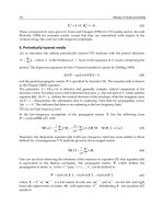
Fig. 2. Propagating and evanescent regions for
qP

and qSV

waves in the


12
,bb domain.
The points

1
1, 1N  and


2
1, 1N denote the crossings between
21
12bb  and
2
21
bb .
The paths corresponding to
f
const


are given for frequencies of 15, 25 and 50
f
Hz

are
shown in magenta, red and blue, respectively. The starting point
0
M
(that corresponds to zero
horizontal slowness) and the points corresponding to crossings of the path and boundaries
between the propagating regions,
,1,2,3
j
Mj , are shown for the frequency
15
f
Hz
.
Points
4
M
and
5
M
are outside of the plotting area (Roganov&Stovas, 2011).
All envelopes are propagating, if the roots of quadratic equation

2
12
20ybyb


 (75)
are such that
1
1y

and
2
1y

. On the boundaries between propagating and evanescent
envelopes, we have
1y


or discriminator of equation (75),

2
12
,0Dp b b


. In the
first case we have,
21
12bb

 , and in the second case,
2
21

bb

(Figure 2). If 1y  , the
equation


cosyH


 has the following solutions

Acoustic Waves in Layered Media - From Theory to Seismic Applications

17




2
2
1
2ln 1,,1
1
(2 1) ln 1 , , 1
ni y y n y
H
niyy ny
H






     







Z
Z
, (76)
and
Req const

 in this area. The straight lines
21
12bb 
and the parabola
2
21
bb
defined between the tangent points


1
1,1N  and



2
1,1N split the coordinate plane


12
,bb
into five regions (Figure 2). If parameters
1
b and
2
b are such that the corresponding point


12
,bb is located in region 1 or 2, the system of equations (74) has no real roots, and
corresponding envelopes do not contain the propagating wave modes. The envelopes with
one propagating wave of qP-or qSV- wave mode correspond to the points located in region
3 or region 4, respectively. The points from region 5 result in envelopes with both
propagating qP- and qSV-wave modes. If a specific frequency is chosen, for instance,
30 Hz


 (or 15
f
Hz

), and only the horizontal slowness is varied, the point with
coordinates



12
,bb will move along some curve passing through the different regions.
Consequently, the number of propagating wave modes will be changed. In Figure 2, we
show using the points
i
M



0, 5i   with the initial position
0
M
defined by 0p  and the
following positions crossing the boundaries for the regions occurred at
1
0.172
p
skm
,
2
0.217pskm and
3
0.246pskm

. This curve will also cross the line
21
12bb  at
4
0.332pskm and

5
0.344pskm

. Between the last two points, the curve is located in the
region 2 with no propagating waves for both modes. The frequency dependent positions of
the stop bands for pconst

can be investigated using the curve,


12
,bbb







.
Since the propagator in the zero frequency limit is given by the identity matrix,

0
lim



PI, than





12
001bb

 , and all curves


b

start at the point


2
1,1N . For
propagating waves, the functions


1
b

and


2
b

are given by linear combinations of
trigonometric functions and therefore are defined only in a limited area in the


12
,bb
domain.

-1.0 -0.5 0.0 0.5 1.0
-1.0
-0.5
0.0
0.5
1.0
cos(

P
)
cos(

S
)
-1.0 -0.5 0.0 0.5 1.0
-1.0
-0.5
0.0
0.5
1.0
b
2
b
1

Fig. 3. The normal incidence case (

0p

). The dependence of


cos
qP
H


on

cos
qSV
H


(a Lissajous curve) is shown (left) and similar curve is plotted in the


12
,bb domain (right).
Both of these plots correspond to frequency range
050Hz

. Note, that the stop bands exist
only for
qP 
wave and can be seen for



cos 1
qP
H

 in the left plot and for
21
12bb  in the right one (Roganov&Stovas, 2011).

Waves in Fluids and Solids

18
The simplest case occurs at the normal incidence where
0p

. At this point the quadratic
equation




2
12
20ybyb

 has two real roots


qP
y


and


qSV
y

for each value
of

. The functions



cos
qP qP
yH

 and



cos
qSV qSV
yH

 are the right side of
the dispersion equation for qP- and qSV- wave, respectively. If these trigonometric
functions have incommensurable periods, the parametric curve
 



,
qSV qP
yy


densely
fills the area that contains rectangle
1,1 1,1

 

 
and is defined as a Lissajous curve
(Figure 3, left). The mapping

,,
2
qSV qP
qSV qP qSV qP
yy
yy yy






has the Jacobian

2
qSV qP
yy




with a singularity at
qSV qP
yy

. This point is located at the discriminant
curve,
2
21
bb . We can prove that the curve




 
,
2
qSV qP
qSV qP
yy
yy









is tangent
to parabola
2
21
bb at the singular point and is always located in the region
2
21
bb . In fact,
if,





1
2
qSV qP
yy
b





,







2 qSV qP
byy


 and


00qP qSV
yy


 than
   


2
2
12 0
1
0
4
qP qSV
bb y y



  
. In Figure 3 (left), it is shown the
parametric curve
 


,
qSV qP
yy


computed for our two layer model described in Table 1.
Since both layers have the same vertical shear wave velocity and density,

cos
qSV qSV
yt

 with


12 0qSV
thh

 . In the qP- wave case,










2
12 12
cos cos 1
qP qP qP qP qP
yttrttr
 
where
1101qP
th


,
2202qP
th


and




02 01 01 02
r



 
. The solutions of this equation and has been studied by Stovas
and Ursin (2007) and Roganov and Roganov (2008). The plot of this curve in


12
,bb domain
is shown in Figure 3 (right). It can be seen that the stop bounds are characterized by the
values
21
12bb  . If


,0Dp


, equation (64) has the complex conjugate and dual roots.
Let us denote one of them as
1
y

C . Then, equation (74) has four complex roots:

,

 ,
*

and
*


 , where


1
cos Hy


. In these cases, the energy envelope equals zero. The up
going and down going wave envelopes have different signs for
Im



that correspond to
exponentially damped and exponentially increasing terms.
6.2 Computational aspects
The computation of the slowness surface at different frequencies is performed by computing
the propagator matrix (15) for the entire period and analysis of eigenvalues of this matrix.
To define the direction for propagation of the envelope with eigenvectors

313331
,,,
T
vv

b
and non-zero energy is done in accordance with sign of the vertical energy flux (Ursin, 1983;
Carcione, 2001)


**
113 3 33
1
Re
2
Evv


 
. (77)

Acoustic Waves in Layered Media - From Theory to Seismic Applications

19
If
0E  , the direction of the envelope propagation depends on the absolute value of


exp iH


;


exp 1iH

 (up going envelope) and



exp 1iH


(down going
envelope). The mode of envelope can be defined by computing the amplitude propagators

1
11

QEPE. (78)
The absolute values of the elements of the matrix
Q are the amplitudes of the different
wave modes composing the envelope and defined in the first layer within the period.
Therefore, the envelope of a given mode contains the plane wave of the same mode with the
maximum amplitude (when compared with other envelopes).
6.3 Asymptotic analysis of caustics
Let us investigate the asymptotic properties for the vertical slowness of the envelope in the
neighborhood of the boundary between propagating and evanescent waves when
approaching this boundary from propagating region.
If

0
1yp  and
0
0dy dp


 , than in the neighborhood of the point
0
pp


the following
approximation of equation


cosyH


 is valid

22 2
11
2
Hd
dp


, (79)
where
0
dp p p ,
0
d



 and


00

p

 . Therefore,


dOdp

 ,

1ddpO dp

 ,
and the curve


p

at the
0
pp

has the vertical tangent line,


0
lim
pp
ddp



. In the
group space




,
x
tx , it leads to an infinite branch represented by caustic. In the area of
propagating waves, we have


0
lim
pp
ddp



 . Therefore,


() /xp Hd dp


 and







tp H p pxp


. Furthermore, for large values of
x
,




00
tx px H p


. This
fact follows from existence of limit,






0
0
lim
pp
p
p




. As a consequence, every continuous
branch of the slowness surface limited by the attenuation zones (stop bands) results in the
caustic in group space which looks like an open angle sharing the same vertex (Figure 4).
When we move from one point of discontinuity to another in the increasing direction of
p ,
the plane angle figure rotates clockwise since the slope of the traveltime curve
0
dt dx p is
increasing. The case where


0
1yp

 can be discussed in the same manner. If

0
0Dp  ,
than
 


11
cos hbDpbOp

  . Therefore, the asymptotic behavior of


p

as
0
pp is the same as discussed above.
6.4 Low frequency caustics
In Figure 5 we show the propagating, evanescent and caustic regions in
pf

domain for
qP- and qSV- waves ( /2f



). Figure 5 displays contour plots of the vertical energy flux
in the
pf domain for qP- and qSV- waves.
From Figure 5 one can see that the caustic area has weak frequency dependence in the low
frequency range (almost vertical structure for caustic region in


,pf
domain, Figures 5 and
6). This follows from more general fact that for VTI periodic medium,




is even function

Waves in Fluids and Solids

20
0.0 0.1 0.2 0.3 0.4 0.5 0.6
0.0
0.1
0.2
0.3
0.4
0.5
0.6
min x
min q'
Vertical slowness (s/km)
Horizontal slowness (s/km)
02468
0.0
0.5
1.0
1.5
2.0
2.5
3.0
Traveltime (s)
Offset (km)

Fig. 4. Sketch for the stop band limited branch of the slowness surface and corresponding
branch on the traveltime curve. The correspondence between characteristic points is shown
by dotted line (Roganov&Stovas, 2011).
of frequency. Last statement is valid because



y

satisfies the equation (75) and functions
  
cosyH



,


1
b

and


2
b

are even. Therefore,








0 o

 
, (80)
and the slowness surface at low frequencies is almost frequency independent.


Fig. 5. The propagating, evanescent and caustic regions for the
qP

wave (left) and the
qSV  wave (right) are shown in the


,
p
f domain. The regions are indicated by colors:
red – no waves, white – both waves, magenta –
qSV

wave only and blue – caustic
(Roganov&Stovas, 2011).


Fig. 6. The vertical energy flux for
qP

wave (left) and qSV - wave (right) shown in the

,pf

domain. The zero energy flux zones correspond to evanescent waves (Roganov&Stovas, 2011).

Acoustic Waves in Layered Media - From Theory to Seismic Applications

21

0.00.10.20.30.40.50.6
0.0
0.1
0.2
0.3
0.4
0.5
0.6
II
I
III
II
I
breaks of
the slowness surface
Vertical slowness (s/km)
Horizontal slowness (s/km)
f=15Hz
qSV-wave
qP-wave
012345678
0.0
0.5
1.0

1.5
2.0
II
III
II
I
I
Traveltime (s)
Offset (km)
f=15Hz
qSV-wave
qP-wave

Fig. 7. The
qP  and qSV

wave slowness surfaces (left) and the corresponding traveltime
curves (right) corresponding frequency of
15Hz . The branches on the slowness surfaces and
on the traveltime curves are denoted by I, II and III (for the
qSV

wave) and I and II (for
the
qP  wave) (Roganov&Stovas, 2011).

0 102030405060708090
1,75
1,80
1,85

1,90
1,95
2,00
2,05
2,10
2,15
breaks of
the slowness surface
Phase velocity (km/s)
Phase angle (degrees)
0 102030405060708090
3,5
3,6
3,7
3,8
3,9
4,0
4,1
breaks of
the slowness surface
Phase velocity (km/s)
Phase angle (degrees)

Fig. 8. The phase velocities for
qSV

wave (left) and qP

wave (right) computed for a
frequency of

15Hz (Roganov&Stovas, 2011).

0,0 0,1 0,2 0,3 0,4 0,5 0,6
0,0
0,1
0,2
0,3
0,4
0,5
0,6
Vertical slowness (s/km)
Horizontal slowness (s/km)
15Hz
25Hz
50Hz
0,6 0,7 0,8 0,9 1,0
0,60
0,62
0,64
0,66
Traveltime (s)
Offset (km)
15Hz
25Hz
50Hz

Fig. 9. Comparison of the
qSV

slowness surface and traveltime curves computed for

frequencies of
15, 25 and 50
f
Hz (shown in magenta, red and blue colors, respectively)
(Roganov&Stovas, 2011).

Waves in Fluids and Solids

22
0,15 0,20 0,25 0,30 0,35
0,30
0,35
0,40
0,45
0,50
Vertical slowness (s/km)
Horizontal slowness (s/km)
LF limit
HF limit
15Hz
0,80 0,85 0,90 0,95 1,00 1,05
0,61
0,62
0,63
0,64
0,65
0,66
0,67
0,68
Traveltime (s)

Offset (km)
LF limit
HF limit
15Hz

Fig. 10. Comparison of the
qSV

slowness surfaces and traveltime curves computed for
frequencies of 15, low and high frequency limits (shown in black, red and blue,
respectively). Note, the both effective media in low and high frequency limits have
triplications for traveltime curves (Roganov&Stovas, 2011).
To illustrate the method described above we choose two-layer transversely isotropic
medium with vertical symmetry axis which we used in our previous paper (Roganov and
Stovas, 2010). The medium parameters are given in Table 1. Each single VTI layer in the
model has its own qSV- wave triplication. In Figure 7 (left), we show the slowness surfaces
for the qP- and qSV- waves computed for a single frequency of 15 Hz. The discontinuities in
both slowness surfaces correspond to the regions with evanescent waves or zero vertical
energy flux,
0E  (equation (77)). The first discontinuity has the same location on the
slowness axis for both qP- and qSV- wave slowness surfaces. In the group space (Figure 7,
right), we can identify each traveltime branch with correspondent branch of the slowness
surface. In Figure 8, we show the phase velocities for qP- and qSV- waves versus the phase
angle

. The discontinuities in the phase velocity are clearly seen for both qP- and qSV-
waves in different phase angle regions. Comparisons of the qSV- wave slowness surface and
traveltime curves computed for different frequencies, 15,25f

and 50Hz are given in

Figure 9. One can see that higher frequencies result in more discontinuities in the slowness
surface. Only the branches near the vertical and horizontal axis remain almost the same. In
Figure 10, we show the slowness surfaces and traveltime curves computed for frequency
15
f
Hz and those computed in the low and high frequency limits. The vertical slowness
and traveltime computed in low and high frequency limits are continuous functions of
horizontal slowness and offset, respectively.
7. Reflection/transmission responses in periodicaly layered media
The problem of reflection and transmission responses in a periodically layered medium is
closely related to stratigraphic filtering (O’Doherty and Anstey,1971; Schoenberger and
Levin, 1974; Morlet et al., 1982a, b; Banik et al., 1985a, b; Ursin, 1987; Shapiro et al., 1996;
Ursin and Stovas, 2002; Stovas and Ursin, 2003; Stovas and Arntsen, 2003). Physical
experiments were performed by Marion and Coudin (1992) and analyzed by Marion et al
(1994) and Hovem (1995). The key question is the transition between the applicability of
low- and high-frequency regimes based on the ratio between wavelength (

) and thickness
( d ) of one cycle in the layering. According to different literature sources, this transition

Acoustic Waves in Layered Media - From Theory to Seismic Applications

23
occurs at a critical
d

value which Marion and Coudin (1992) found to be equal to 10.
Carcione et al. (1991) found this critical value to be about 8 for epoxy and glass and to be 6 to 7
for sandstone and limestone. Helbig (1984) found a critical value of
d


equal to 3. Hovem
(1995) used an eigenvalue analysis of the propagator matrix to show that the critical value
depends on the contrast in acoustic impedance between the two media. Stovas and Arntsen
(2003) showed that there is a transition zone from effective medium to time-average medium
which depends on the strength of the reflection coefficient in a finely layered medium.
To compute the reflection and transmission responses, we consider a 1D periodically
layered medium. Griffiths and Steinke (2001) have given a general theory for wave
propagation in periodic layered media. They expressed the transmission response in terms
of Chebychev polynomials of the second degree which is a function of the elements of the
propagator matrix for the basic two-layer medium. They also provided an extensive
reference list.
7.1 Multi-layer transmission and reflection responses
We consider one cycle of a binary medium with velocities
1
v and
2
v , densities
1

and
2


and the thicknesses
1
h
and
2
h as shown in Figure 11. For a given frequency

f
the phase
factors are:
22
kkk k
f
hv ft
 
, where
k
t

is the traveltime in medium k for one cycle.
The normal incidence reflection coefficient at the interface between the layers is given by

22 11
22 11
vv
r
vv







. (81)
The amplitude propagator matrix for one cycle is computed for an input at the bottom of the
layers (Hovem, 1995)

1 2
1 2
**
2
11
00
1
11
1
00
ii
ii
rrab
ee
rrba
r
ee








   
   

   


Q , (82)
and







12 2 12 2
1
22
2
2
222
11
2sin
,
111
.
iiii
i
ere ree
ir
ab e
rrr
   



 



(83)
We also compute the real and imaginary part of
a
(Brekhovskikh, 1960) and absolute value
of
b , resulting in

v
2

2
v
1

1
d
d
2
d
1

Fig. 11. Single cycle of the periodic medium (Stovas&Ursin, 2007).

Waves in Fluids and Solids

24



2 2
12 12 1 2 12
2 2
2 2
12 12 1 2 12
2 2
2
2
21
Re cos sin sin cos cos sin sin
11
21
Im sin cos sin sin cos cos sin
11
2sin
1
rr
a
rr
rr
a
rr
r
b
r







  


  



(84)
We note, that
22
det 1ab

Q as shown also by Griffiths and Steinke (2001). The
amplitude propagator matrix can be represented by the eigenvalue decomposition (Hovem,
1995)

1

QEΣ E , (85)
where


12
,diag



Σ with



2
1,2
2
Re 1 Re Re 1
Re Re 1 Re 1
ai a for a
aa fora












(86)
and the matrix


12
11
ab ab







E (87)

A stack of M cycles of total thickness


12
DMhMhh  has the propagator matrix



122 221 2 1
1
22 21 21 22 2 1 2 22 1 21
1
MM MM
MM
MM M M
uu
M
uu uu u u
 
  



 
  



QQEΣ E
(88)

with

21 1
uab

 and


22 2
uab

 . Another way to compute the propagator or
transfer matrix is to exploit the Cailey-Hamilton theorem to establish relation between
2
Q
and
Q (Wu et al., 1993) which results in the recursive relation for Chebychev polynomials.
The transmission and reflection responses for a down-going wave at the top of the layers are
(Ursin, 1983)






21
1 1
21
22 12 22
2211 2211
,
MM
D D
MM MM
b
tp rpp
aa aa



    
 


  
 
(89)
with
,, 1,2
ij
pij being the elements of propagator matrix



M
Q given in (88). After
algebraic manipulations equation (89) can be written as

Acoustic Waves in Layered Media - From Theory to Seismic Applications

25


1
2
2
2
2
2
Im
cos sin
sin
sin
sin cos Im sin
Im
1
1sin 1
sin
sin sin
sin cos Im sin sin
1
i
D
i

D D
a
MiM
e
t
MiaM
a
C
M
bM M Ce
rtb
MiaM
C






 



  
















, (90)
where

and C are the phase and amplitude factors, respectively, and

is the phase of
the eigen-value. The equation for transmission response in periodic structure was
apparently first obtained in the quantum mechanics (Cvetich and Picman, 1981) and has
been rediscovered several times. For extensive discussion see reference 13 in Griffiths and
Steinke (2001). The reflection and transmission response satisfy

22
1
DD
tr

 , (91)
which is conservation of energy. When
Re 1a  , the eigen-values give a complex phase-
shift, representing a propagating regime. Then equation (86) gives

1,2
i
e



 (92)
with
cos Re a

 , which may be obtained from Floquet solution for periodic media, but for
first time appeared in Brekhovskikh (1960), equation (7.25). Then we use

2
cos sin
cos
sin
1
,
M
M
Cb
C






, (93)

in equation (90). Equation (93) for the amplitude factor is given in a form of Chebychev
polynomials of the second kind written in terms of sinusoidal functions. When
Re 1a  ,
the eigen-values are a damped or increasing exponential function, representing an
attenuating regime. Then equation (86) gives

1,2
e




(94)
with
cosh Re a

 . Then the reflection and transmission responses are still given by
equation (90) but with phase and amplitude factors now given by

2
cosh sinh
cos
sinh
1
,
M
M
Cb
C







, (95)
For the limiting cases with
Re 1a

, there is a double root

1,2
Re a


(96)

Waves in Fluids and Solids

26
and then we must use

2
2
1
cos
1
, CbM
bM




(97)
Note, that in this case

22
Imba . To compute expressions (93) and (95) for even number
M
we use (Gradshtein and Ryzhik, 1995, equation 1.382)





2
2 2
2 2
2
2 2
1 1
11Re 1Re
cos 1 Re 1
21
1
sin sin
2
,
M M
k k
aa

CbM a
kk
C
M
M



 

  


 
 
 
 
 

(98)
The transmission response from equation (84) can be expressed via the complex phase factor



:




i

D
te



(99)
with

 

2
1
ln 1
2
iC
 
 
. (100)
The angular wavenumber is denoted k . With


RekD


 or

cos coskD


 , the

phase velocity is given by





vkD


 . (101)
Using notations from Carcione (2001), the dispersion equation can be written as



,coscos 0Fk kD

 , and the expression for group velocity is



Fk D
V
F


 

 

 

. (102)
7.2 Equivalent time-average and effective medium
The behaviour of the reflection and transmission responses is determined by
Re a which is
one for
0f 
. The boundaries between a propagating and attenuating regime are at
Re 1a  (see equation (84)) given by the equation

12
1
tan tan
221
r
r




. (103)
For low frequencies the stack of the layers behaves as an effective medium with a velocity
defined by (Backus, 1962; Hovem, 1995) and can be defined as the zero-frequency limit
(

0
EF
vv


from equation (101))

Acoustic Waves in Layered Media - From Theory to Seismic Applications

27

2
12
22 2 2
12
114 1
1
EF TA
hh r
vv hvvr


. (104)

This occurs for frequencies below the first root of the equation Re 1a

 . For higher
frequencies the stack of the layers is characterized by the time-average velocity defined by
the infinite frequency limit (


TA
vv




from equation (101))

12
121 2
11
TA
hh
vhhvv





. (105)

This occurs for frequencies above the second root of the equation Re 1a

 . There is a
transition zone between these two roots in which the stack of layers partly blocks the
transmitted wave.
The behaviour of the medium is characterized by the ratio between wavelength and layer
thickness. This is given by


12
1
TA
v
hfhh ft



 

, (106)

where t is the traveltime through the two single layers. To estimate the critical ratio of
wavelength to layer thickness we assume
12
2ttt . The effective medium limit the
occurs at

1
1
1
tan
1
r
a
r








, (107)

and the time-average limit the occurs at

1
2
1
tan
21
r
a
r









, (108)

For small values of
1r 
we obtain





1
1,2

2
tan 4 1
42
rr
a




 . (109)

The transition between an effective medium to time average medium is schematically
illustrated in Figure 12. Since the boundaries for the transmission zone in equation (103) are
periodic functions of frequency, the low wavelength zone (high frequencies) is more
complicated than shown in this figure.

Waves in Fluids and Solids

28
0,0 0,1 0,2 0,3 0,4 0,5 0,6 0,7 0,8 0,9
0
4
8
12
16
20
24
28
32
36

40
/d
Time average medium
Effective medium
Transition zone
Absolute value of r

Fig. 12. Schematic representation of the critical
d

 ratio as function of reflection
coefficient (
12


 ) (Stovas&Ursin, 2007).
7.3 Reflection and transmission responses versus layering and layer contrast
We use a similar model as in Marion and Coudin (1992) with three different reflection
coefficients: the original
0.87

r
and 0.48r

and 0.16r

. We use
m
and Hz instead of
mm

and kHz . The total thickness of the layered medium is 51
kk
DMh m is constant.
,1,2,4, ,64
k
Mk is the number of cycles in the layered medium, so that the individual layer
thickness is decreasing as k is increasing. The ratio




12 1 2 12 21
0.91tt hv hv

    . The
other model parameters are given in Stovas and Ursin (2007).

0 100 200 300 400 500 600 700
-1
0
1
Frequency [Hz]
-1
0
1
-1
0
1
-1
0

1
-1
0
1
-1
0
1
-1
0
1
M1
M2
M4
M8
M16
M32
M64
r=0.16

0 100 200 300 400 500 600 700
-1
0
1
Frequency [Hz]
-1
0
1
-1
0
1

-1
0
1
-1
0
1
-1
0
1
-1
0
1
M1
M2
M4
M8
M16
M32
M64
r=0.48


0 100 200 300 400 500 600 700
-1
0
1
Frequency [Hz]
-1
0
1

-1
0
1
-1
0
1
-1
0
1
-1
0
1
-1
0
1
M1
M2
M4
M8
M16
M32
M64
r=0.87

Fig. 13. Re a as function of frequency.
Re 1a

is only plotted with area filled under the
curve (Stovas&Ursin, 2007).

Acoustic Waves in Layered Media - From Theory to Seismic Applications

29
0 100 200 300 400 500 600 700
-1,0
-0,5
0,0
0,5
1,0
Frequency [Hz]
-1,0
-0,5
0,0
0,5
1,0
-1,0
-0,5
0,0
0,5
1,0
-1,0
-0,5
0,0
0,5
1,0
-1,0
-0,5
0,0
0,5
1,0

-1,0
-0,5
0,0
0,5
1,0
-1,0
-0,5
0,0
0,5
1,0
M1
M2
M4
M8
M16
M32
M64
r=0.16

0 100 200 300 400 500 600 700
-1,0
-0,5
0,0
0,5
1,0
Frequency [Hz]
-1,0
-0,5
0,0
0,5

1,0
-1,0
-0,5
0,0
0,5
1,0
-1,0
-0,5
0,0
0,5
1,0
-1,0
-0,5
0,0
0,5
1,0
-1,0
-0,5
0,0
0,5
1,0
-1,0
-0,5
0,0
0,5
1,0
M1
M2
M4
M8

M16
M32
M64
r=0.48


0 100 200 300 400 500 600 700
-1,0
-0,5
0,0
0,5
1,0
Frequency [Hz]
-1,0
-0,5
0,0
0,5
1,0
-1,0
-0,5
0,0
0,5
1,0
-1,0
-0,5
0,0
0,5
1,0
-1,0
-0,5

0,0
0,5
1,0
-1,0
-0,5
0,0
0,5
1,0
-1,0
-0,5
0,0
0,5
1,0
M1
M2
M4
M8
M16
M32
M64
r=0.87

Fig. 14. The phase function
cos

as a function of frequency (from equation (98)) shown by
solid line and cos

corresponding to the single layer with time-average velocity shown by
dashed line (Stovas&Ursin, 2007).

The very important parameter that controls the regime is
Re a
(equation (84)). The plots of
Re a versus frequency are given in Figure 13 for different models. One can see that the
propagating and attenuating regimes are periodically repeated in frequency. The higher
reflectivity the more narrow frequency bands are related to propagating regime ( Re 1a  ).
One can also follow that the first effective medium zone is widening as the index of model
increases and reflection coefficient decreases, and that the wavelength to layer thickness
ratio

is the parameter which controls the regime. The gaps between the propagating
regime bands become larger with increase of reflection coefficient. These gaps correspond to
the blocking or attenuating regime. The graphs for the phase factor cos

and amplitude
factor
C (equation (98)) are shown in Figure 14 and 15, respectively. The dotted lines in
Figure 14 correspond to the time-average phase behaviour. One can see when the computed
phase becomes detached from the time-average phase. Note also the anomalous phase
behaviour in transition zones. The amplitude factor
C (Figure 15) has periodic structure,
and periodicity increase with increase of reflection coefficient. In transition zones the
amplitude factor reaches extremely large values which correspond to strong dampening.
The transmission and reflection amplitudes are shown in Figure 16. The larger reflection
coefficient the more frequently amplitudes change with frequency. The transition zones can
be seen by attenuated values for transmission amplitudes. With increase of reflection

Waves in Fluids and Solids

30

0 100 200 300 400 500 600 700
-2
-1
0
1
2
Frequency [Hz]
-2
-1
0
1
2
-2
-1
0
1
2
-2
-1
0
1
2
-2
-1
0
1
2
-2
-1
0

1
2
-2
-1
0
1
2
M1
M2
M4
M8
M16
M32
M64
r=0.16

0 100 200 300 400 500 600 700
-10
-5
0
5
10
Frequency [Hz]
-10
-5
0
5
10
-10
-5

0
5
10
-10
-5
0
5
10
-10
-5
0
5
10
-10
-5
0
5
10
-10
-5
0
5
10
M1
M2
M4
M8
M16
M32
M64

r=0.48


0 100 200 300 400 500 600 700
-20
-10
0
10
20
Frequency [Hz]
-20
-10
0
10
20
-20
-10
0
10
20
-20
-10
0
10
20
-20
-10
0
10
20

-20
-10
0
10
20
-20
-10
0
10
20
M1
M2
M4
M8
M16
M32
M64
r=0.87

Fig. 15. The amplitude function C (from equation (98)) as a function of frequency (very
large values of C are not shown) (Stovas&Ursin, 2007).
coefficient the dampening in transmission amplitudes becomes more dramatic. The exact
transmission and reflection responses are computed using a layer recursive algorithm (Ursin
and Stovas, 2002). We use a Ricker wavelet with a central frequency of 500 Hz. The
transmission and reflection responses are shown in Figure 17 and 18, respectively. No
amplitude scaling was used. One can see that these plots are strongly related to the
behaviour of Re a (Figure 13). The upper seismogram in Figure 17 is similar to the Marion
and Coudin (1992) experiment and the Hovem (1995) simulations. The effects related to the
effective medium (difference between the first arrival traveltime for model
1

M
and
64
M
and
the transition between effective and time average medium, models
416
M
M ) are the more
pronounced for the high reflectivity model. For this model the first two traces (models
1
M

and
2
M
) are composed of separate events, and then the events become more and more
interferential as the thickness of the layers decrease. Model
8
M
gives trains of nearly
sinusoidal waves (tuning effect). The transmission response for model
16
M
is strongly
attenuated, and models
32
M
and
64

M
behave as the effective medium. From Figures 13-16
and the transmission and reflection responses (Figures 17 and 18) one can distinguish
between time average, effective medium and transition behaviour. This behaviour can be
seen for any reflectivity, but a decrease in the reflection coefficient results in the convergence
of the traveltimes for time-average and effective medium. This makes the effective medium
arrival very close to the time average one. Note also that for the very much-pronounced

Acoustic Waves in Layered Media - From Theory to Seismic Applications

31

0 100 200 300 400 500 600 700
0,0
0,5
1,0
M64
M32
M16
M8
M4
M2
M1
r=0.16
Frequency [Hz]
0,0
0,5
1,0
0,0
0,5

1,0
0,0
0,5
1,0
0,0
0,5
1,0
0,0
0,5
1,0
0,0
0,5
1,0

0 100 200 300 400 500 600 700
0,0
0,5
1,0
M64
M32
M16
M8
M4
M2
M1
r=0.48
Frequency [Hz]
0,0
0,5
1,0

0,0
0,5
1,0
0,0
0,5
1,0
0,0
0,5
1,0
0,0
0,5
1,0
0,0
0,5
1,0


0 100 200 300 400 500 600 700
0,0
0,5
1,0
M64
M32
M16
M8
M4
M2
M1
r=0.87
Frequency [Hz]

0,0
0,5
1,0
0,0
0,5
1,0
0,0
0,5
1,0
0,0
0,5
1,0
0,0
0,5
1,0
0,0
0,5
1,0

Fig. 16. The transmission amplitude (solid line) and reflection amplitude (dotted line) as
function of frequency (Stovas&Ursin, 2007).

0,00 0,02 0,04 0,06 0,08 0,10
-4
0
4
M4
M2
M1
r=0.16

Time [s]
-4
0
4

-4
0
4

-4
0
4
M64
M32
M16
M8

-4
0
4

-4
0
4

-4
0
4

0,00 0,02 0,04 0,06 0,08 0,10

-3,5
0,0
3,5
M4
M2
M1
r=0.48
Time [s]
-3,5
0,0
3,5

-3,5
0,0
3,5

-3,5
0,0
3,5
M64
M32
M16
M8

-3,5
0,0
3,5

-3,5
0,0

3,5

-3,5
0,0
3,5



0,00 0,02 0,04 0,06 0,08 0,10
-1
0
1
M4
M2
M1
r=0.87
Time [s]
-1
0
1

-1
0
1

-1
0
1
M64
M32

M16
M8

-1
0
1

-1
0
1

-1
0
1


Fig. 17. Numerical simulations of the transmission response (Stovas&Ursin, 2007).

Waves in Fluids and Solids

32

0,00 0,02 0,04 0,06 0,08 0,10
-1,5
0,0
1,5
Time [s]
-1,5
0,0
1,5

M1
M2
M4
M8
M16
M32
M64
-1,5
0,0
1,5
-1,5
0,0
1,5
-1,5
0,0
1,5
-1,5
0,0
1,5
-1,5
0,0
1,5
r=0.16
0,00 0,02 0,04 0,06 0,08 0,10
-3
0
3
Time [s]
-3
0

3
M1
M2
M4
M8
M16
M32
M64
-3
0
3
-3
0
3
-3
0
3
-3
0
3
-3
0
3
r=0.48


0,00 0,02 0,04 0,06 0,08 0,10
-4
0
4

Time [s]
-4
0
4
M1
M2
M4
M8
M16
M32
M64
-4
0
4
-4
0
4
-4
0
4
-4
0
4
-4
0
4
r=0.87

Fig. 18. Numerical simulations of the reflection response (Stovas&Ursin, 2007).
effective medium (model

64
M
,
0.87

r
) one can see the effective medium multiple on the
time about 0.085s. The reflection responses (Figure 18) demonstrate the same features as the
transmission responses (for example strongly attenuated transmission response is related to
weak attenuated reflection response). Effective medium is represented by the reflections
from the bottom of the total stack of the layers. The phase velocities are computed from the
phase factor (equation (100)) and shown in Figure 19 as a function of frequency. The phase
velocity curve starts from the effective medium velocity and at the critical frequency it
jumps up to the time-average velocity. One can see that the width of the transition zone is
larger for larger values of reflection coefficient. The difference between the effective medium
velocity and time-average velocity limits also increases with reflection coefficient increase.
In Figure 20, one can see time-average velocity, effective medium velocity, phase velocity
(equation (100)) and group velocity (equation (102)) computed for reflection coefficients 0.16,
0.48 and 0,87 and model
64
M
. In this case we are in the effective medium zone. The larger
reflection coefficient is, the lower effective medium velocity, the larger difference between
the phase and group velocity and the velocity dispersion becomes more pronounced. The
effective medium velocity limit also depends on the volume fraction (


212
hhh


) for
one cycle (see equation (104)). This dependence is illustrated in Figure 21 for different values
of reflection coefficient. The maximum difference between the time-average and effective
medium velocity reaches 2.191 km/s at
0.18


(
0.87

r
), 0.513 km/s at 0.24


( 0.48r  )
and 0.053 km/s at
0.26


( 0.16r

). One can see that for the small values of reflection
coefficient the difference between the time-average velocity (high-frequency limit) and
effective medium velocity (low frequency limit) becomes very small. For large values of
reflection coefficient and certain range of volume fraction the effective medium velocity is

Acoustic Waves in Layered Media - From Theory to Seismic Applications

33
0 100 200 300 400 500 600 700

3600
3800
4000
4200
M64
M32
M16
M8
M4
M2
M1
V
EF
V
TA
r=0.16
Frequency [Hz]
0 100 200 300 400 500 600 700
2800
3200
3600
4000
4400
4800
M64
M32
M16
M8
M4
M2

M1
V
EF
V
TA
r=0.48
Frequency [Hz]


0 100 200 300 400 500 600 700
1500
3000
4500
6000
M64
M32
M16
M8
M4
M2
M1
V
EF
V
TA
r=0.87
Frequency [Hz]

Fig. 19. The phase velocity (equation (101)) in m/s as function of frequency (Stovas&Ursin,
2007).

smaller than the minimum velocity of single layer constitutes. The effective medium is related
to the propagating regime. The effective medium velocity depends on the reflection coefficient.
The lesser contrast the higher effective medium velocity (the more close to the time-average
velocity). One can also distinguish between effective medium, transition and time average
frequency bands (Figure 22). These bands are separated by the frequencies given by conditions
from the first two roots of equation
Re 1a

 . The first root (equation (107)) gives the limiting
frequency for effective medium. The second one (equation (108)) gives the limiting frequency
for time average medium. From Figure 22, one can see that the transition zone converges to the
limit
4

 with decreasing reflection coefficient. The first transition zone results in the most
significant changes in the phase velocity and the amplitude factor
C .
8. High-frequency caustics in periodically layered VTI media
The triplications (caustics) in a VTI medium can also be observed for high-frequencies. They
are physically possible for qSV-wave propagation only. The qSV-wave triplications in a
homogeneous transversely isotropic medium with vertical symmetry axis (VTI medium)
have been discussed by many authors (Dellinger, 1991; Schoenberg and Daley, 2003;
Thomsen and Dellinger, 2003; Vavrycuk, 2003; Tygel and et. 2007; Roganov, 2008). The
condition for incipient triplication is given in Dellinger (1991) and Thomsen and Dellinger
(2003). According to Musgrave (1970), we consider axial (on- axis vertical), basal (on-axis
horizontal) and oblique (off-axis) triplications. He also provided the conditions for
generation of all the types of triplications. The approximate condition for off-axis triplication
is derived in Schoenberg and Daley (2003) and Vavrycuk (2003). The condition for on-axis
triplication in multi-layered VTI medium is shown in Tygel et al. (2007).

Waves in Fluids and Solids

34
0 100 200 300 400 500 600 700
800
1200
1600
2000
2400
2800
3200
3600
4000
V
TA
V
EF
(r=0.87)
V
EF
(r=0.48)
V
EF
(r=0.16)
r = 0.16
r = 0.48
r = 0.87
Velocity [m/s]
Frequency [Hz]
0,00,10,20,30,40,50,60,70,80,91,0

2000
2500
3000
3500
4000
4500
5000
5500
Velocity [m/s]
Volume fraction
Time-average velocity
Effective medium velocity
r=0.16
r=0.48
r=0.87


0,00,20,40,60,81,0
0
100
200
300
400
500
600
0
100
200
300
400

500
600
Time average medium
Time average medium
Time average medium
Transition zone
Transition zone
Effective medium
Re a = -1
Re a = -1
Re a = 1
Re a = -1
Re a = 1
Re a = -1

Frequency [Hz]
Absolute value of reflection coefficient

Fig. 20. The time average velocity (equation (105), solid line), the effective medium velocity
(equation (104)), the phase velocity (equation (101), dashed line) and the group velocity
(equation (102), dotted line) as function of frequency computed for model
64
M
and different
reflection coefficients (Stovas&Ursin, 2007) shown to the left. The time-average velocity
(equation (105)) and effective medium velocity (equation 104) as a function of volume
fraction shown in the middle. Behaviour of the model
4
M
as function of frequency and

reflection coefficient shown to the right.
8.1 qSV- wave in a homogeneous VTI medium
In a homogeneous anisotropic medium, the plane wave with the slowness surface defined
by
()qqp and the normal (, )
p
q is given by



p
xqpht

 . (110)
The envelope of a family of plane waves given in (110) can be found by differentiation of
equation (110) over the horizontal slowness
p




0xqph


 . (111)
Equations (110) and (111) define the parametric offset-traveltime equations in a this medium
at the depth
h and can be written as follows








,
x
phqtphpqq


 , (112)
where qdqdp

 is the derivative of vertical slowness. The condition for triplication
(caustic in the group space or concavity region on the slowness curve) is given by setting the
curvature of the vertical slowness to zero,
0q



, or by setting the first derivative of offset
to zero,
0x


. These points at slowness surface have the curvature equal to zero. If the

Acoustic Waves in Layered Media - From Theory to Seismic Applications

35

triplication region is degenerated to a single point, it is called incipient triplication. At that
point we have 0q



and 0q



. For the incipient horizontal on-axis triplication, it is not
true, because at that point
q

equal to infinity, and we have to take the corresponding limit.
The triplications can be also related to the parabolic points on the slowness surface with one
of the principal curvatures being zero. The exception is the incipient vertical on-axis
triplication with both principal curvatures equal to zero. The phase velocity can be written
(Schoenberg and Daley, 2003) as a function of phase angle



 
2
2
0
2
S
v
vf
g



 , (113)
where
0 S
v is the vertical S-wave velocity, and function


f

is defined as



  

2
2
11 1
PS
f
feugeugEu

, (114)
where + and – correspond to qP- and qSV-wave, respectively, cos 2u


, and parameters
11 33
11 33

cc
e
cc



,
55
11 33
2c
g
cc


and
2
11 55 33 55 13 55
2
11 33
4( )( ) 4( )
()
cccc cc
E
cc



, which can be written
in terms of Thomsen (1986) anisotropy parameters

   
2
0
11211,,eg E eeg
   
     (115)
and
000SP
vv

 is the S- to P-wave vertical velocity ratio. Note, that 01g and
1eg . Parameter E is also known as anelliptic parameter (Schoenberg and Daley,
2003) since it is proportional to the parameter

,
 
2
0
21Eg eg

  
,
which is responsible for the anellipticity of the slowness surface and for the non-
hyperbolicity of the traveltime equation. Vavrycuk (2003) used parameter

to estimate the
critical strength of anisotropy for the off-axis triplications in a homogeneous VTI medium.
For the waves propagating for entire range of the phase angles, it is required that the
function (, )
S

f
uE and the expression under the square-root in equation (114)

22
(, ) (1 ) (1 )
s
uE eu g E u   
(116)
should be non-negative for all ||1u

. Solving equations (, ) 0
S
fuE

and (, ) 0suE  for
the parameter
E , results in the following explicit functions
2
4(1 )
()
1
f
g
eu
Eu
u



and

2
2
(1 )
()
1
s
eu g
Eu
u



, where the sub-indices
f
and
s
indicate the solutions for the
equations 0f  and 0s

, respectively. Function ()
f
Eu defines the minimum plausible
values for the parameter
E in order to satisfy the condition

2
0v

 , while the function
()

s
Eu defines the maximum plausible values for the parameter E in order to satisfy the
condition

2
Im 0v


. By setting derivatives 0
f
dE du

and 0
s
dE du

, we obtain that,

Waves in Fluids and Solids

36
for the range
1u

, implicit functions (, ) 0
S
fuE

and (, ) 0suE


have the maximum and
the minimum at the points
1
A
(from 0f

and 0
f
dE du

) and
2
A
(from 0s  and
0
s
dE du  ), respectively (Figure 21). The coordinates for these points are

22 22
11 22
(1 1 )/, 2(1 1 ), /(1), (1)
AA AA
ueeEgeuegEge        . (117)


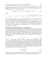
Fig. 21. Schematic plot of the triplication conditions on


,uE space. The graphs for
(, ) 0

S
fuE and (, ) 0su E

are shown by dash line, and the graph for (, ) 0
S
uE

 is
shown by solid line. Points
1
A
and
2
A
correspond to the extrema of the functions
(, ) 0
S
fuE and (, ) 0su E

, respectively. Points
1
B
and
2
B
are the limiting points on the
lower branch of
(, ) 0
S
uE



from the left and from right, respectively. Points
2
A
,
1
C and
2
C correspond to the extrema of the function (, ) 0
S
uE


which has two branches limiting
the triplication areas: 1 – vertical on-axis, 2 – horizontal on-axis and 3 – off-axis. The
condition
12AA
E
EE is a necessary and sufficient condition for existence of qP- and qSV-
waves for entire range of the phase angles (Roganov&Stovas, 2010).
Therefore, the parameter
E is limited as follows
12AA
E
EE . Note, that
1
0
A
u  if 0e  .

The equation for
2A
u was shown in Schoenberg and Daley (2003). The lower limit yields the
condition

2
0v

 , while the upper limit is related to the Thomsen’s (1986) definition of
parameter

, i.e.
2
0
12 0



. The range for parameter E yields a necessary and
sufficient condition for the Christoffel matrix being positive definite for the entire range of
the phase angles. Therefore, this condition is valid for all physically plausible medium
parameters. Using equation (113) and
sin ( ), cos ( ), cos2pVq Vu


,
we obtain that for both types of waves we have the following equalities
p

00
1(1) 1(1)
,
SS
ug ug
pq
vf vf


, (118)
where

P
S
f
f depending on the wave-mode (see equation (114)). The first and second
derivatives of the vertical slowness are given by

Acoustic Waves in Layered Media - From Theory to Seismic Applications

37

/
/
((1))
((1))
u
u
dq p f f u
dp q f f u

 


, (119)

2
2233
0
2
S
dq g
dp v q


 , (120)
where
/
u
f
df du and


 

11 11 ,
PS PS
eg eug E u eg s mns
 
  (121)
with

s
given in equation (116) and










  
 


2 3
22322 2 2 22
2 2
22 2 2 2 2 2 2
2223131112211
11641 1211
mEee ggu e gu e gu g g eg eg eug
nuE eggueguegEgeeug
        
               





. (122)

For qSV and qP waves propagating in a homogeneous VTI medium, the triplication
condition is given by (Roganov, 2008)
(, ) 0
S
uE


, (123)

(, ) 0
P
uE


. (124)
Equations (121)-(122) are too complicated to define the influence of parameters
e
and
g
on
the form of the curves given by equations (123) and (124). Nevertheless, these equations can be
used for numerical estimation of the position for triplications with any given values for
e
and
g
, as well as for the following theoretical analysis. It is well known that qP waves never have
triplications in a homogeneous VTI medium (Musgrave, 1970; Dellinger, 1991; Vavrycuk,
2003), and, therefore, the equation (124) has no roots for propagating qP waves. By taking all

the physically possible values for
u
,
e
,
g
and E , one can prove that if (, ) 0suE  , 1u  ,
01g and 1eg

 , the following inequality always takes place, (, ) 0
P
uE


.
The product of
(, )
P
uE

and (, )
S
uE



22
(, ) (, ) (, )
PS
uE uE uE m sn



(125)
given by polynomial with the sixth order in
u and fifth order in E , can also be used to
define the triplications for qSV-waves. For elliptical anisotropy,
0E

, we have the
equalities
(, ) 2
S
f
uE g and
2
55
()Vc

 . In this case, both the slowness and the group
velocity surfaces are circles, and qSV-waves have no triplications. The straight line given by
0E  , separate the plane (, )uE into sub-planes with non-crossing branches of the curve
(, ) 0
S
uE

 . One of these branches is located in the range of values
1
0
A
EE



and
1u 

and is limited from the left and the right by the points
1
B
and
2
B
, respectively. The
coordinates of these points are (Figure 23)

Waves in Fluids and Solids

38





11 2 2
1, 1 1, 1,
BB B B
uEgegu Egeg        , (126)
while the second branch is closed and located in the range of values
2
0
A

EE . The
limited values
1
0
B
E

and
2
0
B
E

, that follows from inequalities 01g

 and 1eg .
Under the lower branch of the curve
(, ) 0
S
uE


on the plane (, )uE , there are two
parameter areas resulting in the on-axis triplications (both for vertical and horizontal axis),
while the upper branch of the curve (, ) 0
S
uE


defines the parameter area for the off-axis

triplications. In Figure 23, these areas are denoted by numbers 1, 2 and 3, respectively.
Therefore, the on-axis triplications can simultaneously happen for both axis, if 0E  , while
the off-axis triplications can exist only alone, if
0E  . Let us define the critical values for
parameter
E in (, )uE space with horizontal tangent line (
1A
E
,
2A
E
,
1C
E and
2C
E in Figure
23) that define the incipient triplications. In order to do so we need to solve the system of
equations

(, ) 0
(, )
0
S
S
uE
uE
u












. (127)
For the range of parameters
12AA
E
EE and 1u

, system of equations (127) has four
solutions, where the first two solutions


11
,
AA
uE and


22
,
AA
uE are defined above. For
the second two solutions



11
,
CC
uE and


22
,
CC
uE we have
122CC A
uuu, while
1C
E and
2C
E are the largest (always positive) and intermediate (always negative) roots of the cubic
equation











2

322 2 22 22 2
3323 81 161 1 0tE E g e g E g g e E g e g e         
. (128)
Equations similar to our equation (128) are derived in (Peyton, 1983; Schoenberg and Helbig,
1997; Thomsen and Dellinger, 2003; Vavrycuk, 2003; Roganov, 2008). To prove that equation
() 0tE  gives the positions for the critical points of the curve (, ) 0uE

 one can
substitute
2A
uu
. Consequently, we have





2
2
2
22
2
1
(,) ()(,)
1
AA
ge
uE tEpu E
g





(129)
and

2
2
22
(,) 6(1 )
(,)
(1 )
A
A
uE e g
uE
uge





. (130)
Therefore, if
() 0tE

and
2
A
uu , then system of equations (127) is obeyed. The least root

of equation (128) is located in the area defined by 1E

 and holds also equation
(, ) 0
P
uE

 . It is located outside the region
12
A
A
EEE and does not define any qSV
wave triplication. The intermediate root defines the critical point
2
C on the lower branch of
the curve (123). The minimum point
1
A
(dividing the triplication domain 1 and 2) is also