Advances in Mechatronics Part 3 doc

Integrated Control of Vehicle System Dynamics: Theory and Experiment

29
9. Appendix
The acceleration of the vehicle can be expressed by





xyz yxz
avv ivv
j

 

(a1)
where
cos
x
vv


and sin
y
vv


; the above equation can be derived as the following
equation by assuming the vehicle speed

v is constant





sin cos
zz
av iv
j


   

(a2)
Therefore



sin
xz
av


 

(a3)
and



cos
yz
av




(a4)
and hence
cos sin
xy
aa



 (a5)
Combining Eq. (a3) and (a5), the following equation can be easily derived

1
(cos sin)
zy x
aa
v


  

(a6)
When


is small, the following equation can be easily derived from Eq. (a4)

y
z
a
v





(a7)
10. References
Bakker, E, Nyborg, L, and Pacejka, H.B. (1987), Tyre Modeling for Use in Vehicle Dynamics
Studies,
SAE Technical Paper 870421, pp. 2190-2198.
Boada, B.L., Boada, M.J.L., and Diaz, V. (2005), Fuzzy-logic Applied to Yaw Moment Control
for Vehicle Stability,
Vehicle System Dynamics, Vol. 43, pp. 753-770.
Chang, S., and Gordon, T.J. (2007), Model-based Predictive Control of Vehicle Dynamics,
International Journal of Vehicle Autonomous Systems, Vol. 5(1-2), pp. 3-27.
Chen, W.W., Xiao, H.S., Liu, L.Q., and Zu, J.W. (2006), Integrated Control of Automotive
Electrical Power Steering and Active Suspension Systems Based on Random Sub-
optimal Control,
International Journal of Vehicle Design, Vol. 42(3/4), pp. 370-391.
Falcone, P., Borrelli, F., Asgari, J., Tseng, H. E., and Hrovat, D. (2007), Predictive Active
Steering Control for Autonomous Vehicle Systems,
IEEE Transactions on Control
Systems Technology
, Vol. 15(3), pp. 566-580.

Advances in Mechatronics

30
Fruechte, R.D., Karmel, A.M., Rillings, J.H., Schilke, N.A., Boustany, N.M., and Repa, B.S.
(1989), Integrated Vehicle Control,
Proceedings of the 39
th
IEEE Vehicular Technology
Conference
, Vol. 2, pp. 868-877.
Gordon, T.J. (1996), An Integrated Strategy for the Control of a Full Vehicle Active
Suspension System,
Vehicle System Dynamics. Vol. 25, pp. 229-242.
Gordon, T.J., Howell, M., and Brandao, F. (2003), Integrated Control Methodologies for
Road Vehicles,
Vehicle System Dynamics, Vol. 40(1-3), pp. 157-190.
Gu, Z.Q., Ma, K.G., and Chen, W.D. (1997),
Active Control of Vibration (in Chinese), China
National Defense Industry Press, Beijing, China.
He, J.J., Crolla, D.A., Levesley, M.C., and Manning, W.J. (2006), Coordination of Active
Steering, Driveline, and Braking for Integrated Vehicle Dynamics Control,
Proceedings of Institution of Mechanical Engineers - Part D: Journal of Automobile
Engineering
, Vol. 220, pp. 1401-1421.
Hirano, Y., Harada, H., Ono, E., and Takanami, K. (1993), Development of An Integrated
System of 4WS and 4WD by H Infinity Control,
SAE Technical Paper 930267, pp. 79-
86.
Karbalaei, R., Ghaffari, A., Kazemi, R., and Tabatabaei, S.H. (2007), A New Intelligent

Strategy to Integrated Control of AFS/DYC Based on Fuzzy Logic,
International
Journal of Mathematical, Physical and Engineering Sciences
, Vol. 1(1), pp. 47-52.
Li, D.F., Du S.Q., and Yu, F. (2008), Integrated Vehicle Chassis Control Based on Direct Yaw
Moment, Active Steering, and Active Stabiliser,
Vehicle System Dynamics, Vol. 46(1),
pp. 341-351.
Nwagboso, C. O., Ouyang, X., and Morgan, C. (2002), Development of Neural Network
Control of Steer-by-wire System for Intelligent Vehicles,
International Journal of
Heavy Vehicle Systems
, Vol. 9(1), pp. 1-26.
Pacejka, H.B. (2002),
Tyre and Vehicle Dynamics, Butterworth-Heinemann, Boston.
Rodic, A.D., and Vukobratovie, M.K. (2000), Design of an Integrated Active Control System
for Road Vehicles Operating with Automated Highway Systems,
International
Journal Computer Application Technology
, Vol. 13, pp. 78-92.
Trächtler, A. (2004), Integrated Vehicle Dynamics Control Using Active Brake, Steering, and
Suspension Systems,
International Journal of Vehicle Design, Vol. 36(1), pp. 1-12.
Yu F., and Crolla D.A. (1998), An Optimal Self-tuning Controller for An Active Suspension,
Vehicle System Dynamic, Vol. 29, pp. 51-65.
Yu, F., Li, D.F., Crolla, D.A. (2008), Integrated Vehicle Dynamic Control – State-of-the Art
Review,
Proceedings of IEEE Vehicle Power and Propulsion Conference (VPPC),
September 3-5, Harbin, China, pp. 1-6.

2
Integrating Neural Signal and Embedded
System for Controlling Small Motor
Wahidah Mansor, Mohd Shaifulrizal Abd Rani and Nurfatehah Wahy
Universiti Teknologi Mara
Malaysia
1. Introduction
Nowadays, controlling electronic devices without the use of hands is essential to provide a
communication interface for disable persons to have control over their environment and to
enable multi-tasking operation for normal person. Various methods of controlling electronic
devices without the use of hands have been investigated by researchers, for examples sip-
and-puff, electro-oculogram (EOG signals), light emitter and others [Ding et al., 2005,
Kumar et al., 2002; Breau et al., 2004]. In our previous study, EOG signal was found to be
suitable for activating a television using a specific protocol [Harun et al., 2009], however, it
could not be used when a person is not facing the system. Thus, a method that is more
flexible has to be investigated.
The use of neural signals to directly control a machine via a brain computer interface (BCI)
has been studied since 1960s. Using an appropriate electrode placement and digital signal
processing technique, useful information can be extracted from neural signals [Holzner et al,
2009; Jian et al., 2010; Gupta et al., 1996.] One of the events that can be detected from this
signal is eye blink. It can be used as a mechanism to activate and control a machine which
can help disable people to do their everyday routines.
Most BCI systems employs a computer to process neural signals and perform control. Since
portable system offers benefits such as flexibility, mobility and convenience to use, it is more
preferred than a fixed system. An embedded system can be designed to provide portability
feature. To include this feature, a microcontroller is required to control its operation and
provide a communication link between human and machine.
This chapter discusses how neural signal and embedded system can be combined together
to activate a fan connected to a motor. It covers the introduction to neural signal, neural
signal processing, embedded system and EEG based fan system hardware and software.

2. Neural signal
Neural signal or commonly known as electroencephalogram (EEG) is the representation of
electrical activity of the brain. The overall excitation of the brain determines the amplitude
and patterns of the signal. The excitation depends on the activity of the reticular activating
system in the brain stem. The pattern changes markedly between states of sleep and
wakefulness. The EEG signal is divided into five frequency bands; beta, alpha, theta, delta
and gamma. Beta frequency is in the range of 12 Hz – 22 Hz and occurs when the person is
awaken and in the state of alertness. Alpha is in the range of 8 – 13 Hz and is present when a

Advances in Mechatronics

32
person is awaken and relaxed with eyes close. Theta exists in the frequency range of 4 – 8 Hz
when a person is sleepy, already sleep and in the sleep transition. The slowest wave is delta
which is in the frequency range of 0.5 to 4 Hz and is associated with deep asleep. And
finally gamma (22 – 30 Hz) consists of low amplitude & high frequency waves resulting
from attention or sensory stimulation. Figure 1 shows the normal EEG signal of a relaxed
patient. The signal consists of beta waves which lie in the frequency range of 13 to 22 Hz.
Figure 2 shows EEG signal with eye closure and eye opening. The negative amplitude
shows the eyelids closure and positive value shows the opening of eyelids.


Fig. 1. Normal EEG signal when a person is relax.


Fig. 2. Normal EEG signal with eye closure and eye opening.
The recorded EEG signals always contain artifacts which impede the analysis of the signals.
The artifacts include muscle signals, heart signals, eye movements, power line interference,
eye blinks and others. Artifacts in EEG signals typically are characterized by high
amplitudes. Eye blinking artifacts always present in EEG signals since it is difficult to make

the subject open his/her eye for a long time. In some cases, eye blinking artifacts may be
useful and are required as a parameter for activating a system.

Integrating Neural Signal and Embedded System for Controlling Small Motor

33
In EEG signals, eye blinks occur as peaks with relatively strong voltages. Eye blinks can be
classified as short blinks if the duration of blink is less than 200ms or long blinks if it is
greater or equal to 200ms [Bulling et al, 2006]. The amplitude of the peaks varies between
different subjects. They are often located by setting a threshold in EEG and classified for all
activity exceeding the threshold value.
Eye blinks can be classified into three types: reflexive, spontaneous and voluntary. The eye
blink reflexive is the simplest response and does not require the involvement of cortical
structures. Spontaneous eye blinks are those with no external stimuli specified and they are
associated with the psycho-physiological state of the person . The amplitude of spontaneous
eye blink is in the range of -4 to 3 V with duration of less than 400 ms and frequency of
below 5 Hz. The EEG signal obtained when the eyes moved to the right and left is shown in
Figure 3. This signal contains a lot of artifacts caused by spontaneous eye blinking and
eyelid movements as the eyeball moved. The signal obtained from these eye movements are
not suitable for activating a system as the occurrence of eye movements is difficult to detect.
Figure 4 shows EEG with eye movements upward and downwards. This signal consists of
noise which covers the required information to be extracted.


Fig. 3. EEG signal obtained when the eyes are moved to the right and left. [Abd Rani et al., 2009]


Fig. 4. EEG signal with eye movement upwards and downwards.

Advances in Mechatronics

34
Voluntary eye blinking which is intentional blinking due to predetermined condition,
involves multiple areas of the cerebral cortex as well as basal ganglion, brain stem and
cerebella structures. Figure 5 shows the EEG signal with voluntary eye blinks. This EEG
signal has larger amplitude and longer duration (400 -500 ms) compared to that obtained
from spontaneous eye blink. This signal has been filtered which remove the signals above 5
Hz leaving only very clear eye blinking signals. Other artifacts such as 50 Hz power line
interference and noise have also been removed using analogue filtering provided by the
EEG instrument.


Fig. 5. EEG signal for voluntary eye blinking condition.
The suitable event for activating a system is three continuous eye blinks (with a duration of
1.5 to 2.5 seconds between eye closure and opening as they are not present when the subject
is in relax condition [Abd Rani et al., 2009 ]. The duration between the first cycle of eye
opening and closure and the second cycle should be 3 to 4.5 seconds.
3. Neural signal processing
Basically, there are two ways of acquiring the EEG signals from the subjects; invasive and
non-invasive techniques. In the invasive technique, electrodes are implanted in the subject’s
brain and located on the brain surface whereas the non-invasive technique uses electrodes
that are placed on the scalp. In most cases, non-invasive technique is more preferable than
the invasive technique since it is harmless and easy to use. The standard electrode
placement for the non-invasive technique is called International 10-20 system where 10%
and 20% of a measured distance starting from craniometric reference points such as nasion,
inion, left and right pre-auricular points are used to locate the EEG electrodes. The
placement of electrodes for 10-20 system is shown in Figure 6. In this arrangement, a
reference and ground electrodes are placed either on the ear lobe or mastoid.
As mentioned previously, the recorded EEG signals contain artefacts which have to be
removed in order to obtain good morphological signals. Once a clean EEG signal is

obtained, the second stage is to amplify the signal. EEG signal amplitude obtained from the
scalp is very small, range up to 100mV which is difficult to see without amplification. The
signal also has low frequency. It is necessary to analyse the signal to examine the

Integrating Neural Signal and Embedded System for Controlling Small Motor

35
characteristics of the signal and to ensure the noise has been removed. The signal can be
analysed using Fast Fourier Transform (FFT), time-frequency analysis or time scale analysis.
The FFT only gives frequency information of the signal, thus, time-frequency analysis or
spectrogram is normally used to view the frequency at each time point.


Fig. 6. The International 10-20 System of Electrodes Placement. (Redrawn from
[Norani et al., 2010]
The next stage is extracting the underlying information in the signal. Depending on the
purpose of the study, this stage can be feature extraction or event detection as shown in
Figure 7. If the EEG signal is to be used for activating equipment, a simple and an easy way
is to detect an event from the signal, for example eye blinks and use the output which in the
form of pulses to activate the equipment. Classification process is necessary if specific
features are needed to perform the activation. This stage is also called translation process
where the pattern classified is translated into suitable signal to activate equipment.


Fig. 7. EEG signal processing.
4. Embedded system
A computer system that is embedded in an electronic device to perform specific functions is
called embedded system. It forms part of the system and controls one device or many
devices. The main controller in this system is either a microcontroller or digital signal
processing. A microcontroller is a small computer on a single integrated circuit which is

designed to control devices. It consists of CPU, memory, oscillator, watchdog and input
output units on the same chip. The microcontroller is available in wide range from 4 to 64
bits.

Advances in Mechatronics

36
A PIC microcontroller is commonly used in embedded system due to its simplicity and ease
of use. It offers several advantages such as design time saving, space saving and no
compatibility problems. However, it has limited memory size and input/output capabilities.
Figure 8 shows the block diagram of internal architecture of PIC16F877 microcontroller. The
PIC microcontroller is built around Harvard architecture where two memories; one for
program and the other one for data are separated. Separate buses are used for program and
data memories. This eliminates jumping of program code into data or vice versa. PIC
microcontroller uses RAM memory or known as file registers to store data during execution
and a working register called W register to perform arithmetic and logic functions. User
program is stored in the flash program memory and a status register is used to indicate the
status of microcontroller through flag bits such as carry, zero, digit carry flags and others.
PIC16F877 microcontroller has three 8 bits parallel input/ouput ports, 8 channels of analog
inputs and serial outputs.


Fig. 8. Internal architecture of PIC16F877A microcontroller.
5. EEG based fan system incorporating microcontroller
A block diagram of EEG based fan system incorporating microcontroller is shown in Figure
9. It consists of EEG acquisition system, a microcontroller and a motor circuit. Three
electrodes are connected to the EEG acquisition system and located on the subject’s scalp at
frontal, occipital and ear lobe. The EEG acquisition system is responsible for recording the
EEG signals and passing the signals to the microcontroller system. The recorded EEG signal
consists of voluntary and spontaneous eye blinks. Thus, to activate the motor, four seconds

eye blinks in EEG signal is used. The functions of the microcontroller are to process the EEG
signal, detect four-second eye blinks and use the detection results to control the movements
of motor that is connected to a fan. Here, PIC16F877 is used as it can read analogue signal
directly without the need of external analog to digital converter circuit. Three eye blinks

Integrating Neural Signal and Embedded System for Controlling Small Motor

37
within duration of four seconds are used since it is the best technique to activate a system
[Abd Rani et al, 2009].
There are a few ways of connecting a motor to the microcontroller. If a dc motor is used, a
circuit shown in Figure 10 can be implemented. This is a simple circuit which requires 5V
supply to operate. A relay can be used to activate the motor if it is connected to 240V ac
supply. Figure 11 shows the connection of the microcontroller to the devices on the motor
circuit that comprises a transistor, a diode, a relay and a motor.







Fig. 9. Block diagram of EEG based fan system.

Fig. 10. A simple connection of a dc motor to PIC16F877A.

Advances in Mechatronics

38

Fig. 11. Connection of a motor to PIC16F877A for EEG based fan system.
5.1 Controlling software for the EEG based fan system
The PIC microcontroller cannot work without software. A controlling program is required
to read EEG signals from a subject, detect three time eye blinks and activate the motor. A
program written in C language or PIC assembly language can be used to perform the
detection and control operation. The process of detecting three time eye blink and activating
the ac motor is shown in Figure 12. Initially, the program examines whether the EEG signal
amplitude exceeds the maximum threshold voltage, is below minimum threshold voltage or
lies between the threshold voltages. When three eye blinks within duration of four seconds
is detected, the program sends logic 1 to the output of the microcontroller to drive the relay
to activate the motor.
5.2 Examining system functionality
The functionality of the system can be examined in two stages. In the first stage, the
performance of the system in detecting four second eye blink is evaluated. Here, the
recorded EEG signals that are stored in excel file are used. A digital acquisition card is used
as a communication medium between the computer and microcontroller system. The
function of DAQ card is to transfer the recorded EEG signals from the computer to the PIC
microcontroller. A program written in Visual Basic is used to send the EEG signal from the
computer to the microcontroller. To view the EEG signal received at the output of DAQ, an
oscilloscope is placed at one of the DAQ analogue channels. The transmitted EEG signal
displayed on the computer screen is compared with the signal observed on the oscilloscope.
The eye blinks are detected using software written in C language which is programmed on
the microcontroller. In order to view the signal send to the motor, the output of the

microcontroller is connected to the oscilloscope.

Integrating Neural Signal and Embedded System for Controlling Small Motor

39

Fig. 12. Process of activating a motor using eye blink detected from EEG.
In the second stage, the functionality of the motor circuit is tested using a simple routine
shown in Figure 13. A switch is connected to the input of the microcontroller to initiate the
testing. When the switch is turned on, the routine activates the relay that is connected to the
motor. Once it is confirmed that the eye blink detection module and motor activation
routines are working successfully, these routines can be combined together.

Advances in Mechatronics

40
//Program written for PIC programming to run the a motor connected to ac supply.
#include "16F877a.h"
#byte PORTB=0x06
#byte TRISB=0x86
#byte TRISA=0x85
#byte PORTA=0x05
#use delay(clock=400000)

//main function
void main()
{
TRISA = 0x01; //set PORTA to input
PORTA = 0x00; //set RA0-RA7 low
TRISB = 0x00; //set PORTB to output

while(1) // Loop always
{
while(input(PIN_A0)) // Read status of a switch
{
delay_ms(20); // Delay for 20 ms
PORTB = 0x01; // Turn on the fan connected to a motor
}
PORTB = 0x00; // turn off the motor if the switch
// is off
}
}
Fig. 13. A simple routine to test the functionality of the motor.
6. Results and discussions
The EEG signal containing eye blinks observed at the output of DAQ is shown in Fig. 14.
This signal contains three eye blinks and the length of the signal is 4 seconds. The eyelid
closure and opening can be observed clearly through the signal negative and positive
amplitudes.


Fig. 14. EEG signal observed at the output of DAQ. [Wahy et al, 2010]

Integrating Neural Signal and Embedded System for Controlling Small Motor

41
Figure 15 shows the EEG signal with voluntary eye blinks and the pulse obtained when four
second eye blinks is detected. This pulse is observed at the Port B of the PIC16F877A
microcontroller. The motor starts moving once the transistor connected to port B is switched
on.

Fig. 15. Pulses generated at the output of PIC microcontroller when three eye blinks are
detected. [Wahy et al, 2010]
Figure 16 shows the EEG signal when the subject is in relax condition. This EEG signal
contains spontaneous eye blinks which are not detected by the PIC microcontroller. The
amplitude of spontaneous eye blinks is below the threshold value which causes the PIC
ignores them and no pulse is generated at the output.


Fig. 16. EEG with spontaneous eye blinks observed at the output of PIC microcontroller.
[Wahy et al, 2010]
7. Conclusion
A system that can activate a fan using EEG signal detected by a microcontroller has been
described in this paper. The results showed that eye blinks can be detected successfully
using PIC16F877A. With a program running on PIC16F877 microcontroller, a simple motor

Advances in Mechatronics

42
can be activated using neural signal. This application is suitable for people who cannot
move their hands or the whole body to control a fan. Using this system, users can control a
fan easily without any conventional remote controller. This system is useful for elderly
people and disable persons as well as able-bodied people.
For future work, wireless electrodes should be employed in this system. The purpose is to
make the users to feel comfortable with no wires hanging on their head. With wireless
connection, the microcontroller module can be located at a distance from the user which
provides more freedom for normal person to move around. However, this system requires
intelligent software to eliminate interference and prevent false detection.
8. Acknowledgment
The authors would like to thank Universiti Teknologi MARA, Shah Alam, Malaysia for

providing facilities to carry out this research project.
9. References
Abd Rani, M. S. ; Mansor, W.; Detection Of Eye Blinks From EEG Signals For Home Lighting
System Activation, Proc of International Symposium on Mechatronics and Its
Applications, pp 1- 4, ISBN 978-1-4244-3480-0, Sharjah, UAE, March 24-26, 2009
Bulling, A; Ward, J. A.; Gellersen, H; Troster, G.; Eye Movement Analysis for Activity
Recognition Using Electroculography, IEEE Transaction on Pattern Analysis and
Machine Intelligence, Vol. (33), No. 4, (April 2011), pp. 2006, ISSN 0162-8828
Breau, F.; Marsden, B.; McCluskey, J.; Ellwood, R. J.; Lewis, J.; Light Activated Position
Sensing Array for Persons with Disabilities, Proceedings of IEEE on Bioengineering,
ISBN 0-7803-8285-4 , pp 204-205, April 17-18, 2004
Ding, Q.; Tong, K., Li, G.; Development of an EOG (Electro-Oculography) Based Human-
Computer Interface, Proceedings of IEEE EMBS, Shanghai, China, ISBN 1-4244-0032-
5, pp. 6829-6831, Aug 30 – Sept 3, 2006
Harun, H. and Mansor, W.; EOG Signal Detection for Home Appliances Activation”, IEEE
Colloquium on Signal Processing and Its Applications, Kuala Lumpur, Malaysia, ISBN
978-1-4244-4151-8, pp 195-197, March 6-8, 2009
Kumar, D. and Poole, E.; Classification of EOG for Human Computer Interface, Proceedings
of IEEE EMBS/BMES, USA, ISBN 0-7803-7612-9, pp 64–67, 2002
Norani, N.A.M.; Mansor, W.; Khuan, L.Y.; A review of Signal Processing in brain computer
interface system, Proceedings of IEEE on Biomedical Engineering and Sciences, ISBN
978-1-4244-7599-5, pp 443 – 449, Nov 30 – Dec 2, 2010.
Wahy, N.; Mansor, W.;EEG Based Home-lighting System, Proceedings of IEEE on Computer
Applications and Industrial Electronics, ISBN 978-1-4244-9054-7, pp 379-381, Dec 5-8,
2010.
3
Artificial Intelligent Based Friction Modelling
and Compensation in Motion Control System
Tijani Ismaila B., Rini Akmeliawati and Momoh Jimoh E. Salami
Intelligent Mechatronics Systems Research Unit,

Department of Mechatronics Engineering,
International Islamic University Malaysia
Kuala Lumpur,
Malaysia
1. Introduction
The interest in the study of friction in control engineering has been driven by the need for
precise motion control in most of industrial applications such as machine tools, robot
systems, semiconductor manufacturing systems and Mechatronics systems. Friction has
been experimentally shown to be a major factor in performance degradation in various
control tasks. Among the prominent effects of friction in motion control are: steady state
error to a reference command, slow response, periodic process of sticking and sliding (stick-
slip) motion, as well as periodic oscillations about a reference point known as hunting when
an integral control is employed in the control scheme. Table 1 shows the effects and type of
friction as highlighted by Armstrong et. al. (1994). It is observed that, each of task is
dominated by at least one friction effect ranging from stiction, or/and kinetic to negative
friction (Stribeck). Hence, the need for accurate compensation of friction has become
important in high precision motion control. Several techniques to alleviate the effects of
friction have been reported in the literature (Dupont and Armstrong, 1993; Wahyudi, 2003;
Tjahjowidodo, 2004; Canudas, et.al., 1986).
One of the successful methods is the well-known model-based friction compensation
(Armstrong et al., 1994; Canudas de Wit et al., 1995 and Wen-Fang, 2007). In this method,
the effect of the friction is cancelled by applying additional control signal which generates a
torque/force. The generated torque/force has the same value (or approximately the same)
with the friction torque/force but in opposite direction. This method requires a precise
modeling of the characteristics of the friction to provide a good performance. Hence, in the
context of model-based friction compensation, identification of the friction is one of the
important issues to achieve high performance motion control.
However, as discussed in the literatures, several types of friction models have been
identified (Armstrong et al., 1994; Canudas et. al., 1995; Makkar et. al., 2005) and classified
as static or dynamic friction models. Among the static models are Coulomb friction model,

Tustin model, Leuven model, Karnop model, Lorentzian model. Meanwhile Dahl model,
Lugre model, Seven parameters model, and the most recent Generalized Maxwell-Slip (GMS)
model, are among the dynamic friction models (Tjahjowidodo, 2004). The static friction
model is simple and easy in the identification process, however using such model

Advances in Mechatronics

44
Tasks Friction Effects Dominant Friction
Regulator (pointing/position
control)
Steady-state error, hunting Stiction
Tracking with velocity reversal
Standstill, and lost of
motion
Stiction
Tracking at low velocity Stick-slip
Stribeck friction,
stiction
Tracking at high velocity Large tracking error
Viscous behavior of
lubricant
Table 1. Control tasks and associated friction effects
for friction compensation usually lead to poor performance especially at very low velocity
control.
On the other hand, the accuracy of the dynamic friction model is anchored on the dependency
of friction on immeasurable internal states such as velocity and position. Since friction model
selection is an essential factor in the model-based friction compensation, it is important to find
an appropriate friction model that will effectively alleviate the frictional effects in motion
control applications. This has been the basis for the continuous search for more efficient and

simple model for friction identification and compensation in motion control system.
The recent development in Artificial Intelligent (AI) makes it adaptable for system modeling
base on the data training and expert knowledge. It has been shown that the major AI
paradigms (Neural Network, Fuzzy Logic, Support vector machine etc.) have the capability of
approximating any nonlinear functions to a reasonable degree of accuracy; and hence, have
been identified and proposed as appropriate alternatives for friction model and compensation
in motion control systems, (Bi et.al., 2004; Kemal and Masayoshi, 2007; Wahyudi and Ismaila,
2008). In addition, the use of artificial intelligence based friction model may also reduce both
the complexity and time consumed in the friction modeling and identification.
This chapter first presents an overview of model-based friction techniques which have been
used in friction modeling and compensation in motion control systems. Then the application
of artificial intelligent based methods in this area is reviewed. The development,
implementation and performance comparison of Adaptive Neuro-Fuzzy inference system
(ANFIS) and Support Vector Regression (SVR) for non-linear friction estimation in a motion
control system so as to achieve high precision performance are described. These two AI
techniques are selected based on their unique characterstics over others as discussed latter in
this paper. A comparative study on the performance of these two AI techniques in terms of
modeling accuracy, compensation efficiency, and computational time is examined. The
chapter is concluded with highligths of summary of the results of the study and future
directions of research in this area.
2. Review of friction modelling techniques in motion control system
The study of friction is dated back to the work of Leonardo da Vinci (1452-1519) who
investigated the nature of friction and proposed the basis for the theory of classical friction.
According to da Vinci (1452-1519) theory of friction, and latter work of Amontons (1699),
and Charles (1785) friction is proportional to load, opposed motion, and is independent of

Artificial Intelligent Based Friction Modelling and Compensation in Motion Control System

45
contact area. With the birth of tribology and its recent advancement, details about the

topography of contact between bodies especially at atomic level have been more detailed
and investigated by Armstrong (1991) and recently revisited by Farid (2008).
Two main regimes have been identified for friction, namely: pre-sliding and sliding. Pre-
sliding regime defines friction at very low velocity prior to sliding motion and is a function
of displacement, while sliding regime covers the period when the body is sliding/in motion
and during this period friction is a function of velocity of motion. Some of the challenges in
friction model includes the merging of friction model in both regimes in order to offer a
smooth transition from pre-sliding to sliding regime whichtakes into consideration frictional
effects such as: Stribeck, stick-slip, hysteresis, break-away force, nonlocal memory, and
friction lag. For motion control applications, friction study is been carried out to compesate
its negative effects on control performances.
Several methods have been adopted for friction compensation in the research domain and
industry. Detailed review was given by Armstrong (1994). Non-model-based compensation
includes the use of stiff proportional-derivative (PD) control, integral control with
deadband, dither, impulsive control and joint torque control and nonlinear controllers. Stiff
PD approach involves the use of either high derivative (velocity) feedback or high
proportional position feedback. This has been shown to be effective for stable tracking and
for system designed for high rigidity.
The use of integral control to eliminate the steady state error due to friction is confronted
with the problem of limit cycles. This necessitates the introduction of deadband at the input
of the integrator control block, thereby limiting the attainable steady state accuracy (Shen
and Wang, 1964).
Dither isa high frequency signal added to the control signal to eliminate the effects of the
nonlinearities which include friction in the system. The application of dither in aerospace
control was reported by Oppelt (1976). The challenges in application of dither lies in its
mode of generation and application.
Others form of non-model based techniques include impulsive control, joint torque
(Armstrong, 1992; Hashimoto et.al., 1992).
The use of nonlinear controllers has also been reported by many researchers. PD controller
plus a discontinuous nonlinear proportional feedback (DNPF) was proposed by Southward

et.al.,(1991), while PD plus smooth robust nonlinear feedback (SRNF) was investigated by
Cai and Song (1993). A compensation scheme using nominal characteristic trajectory
following (NCTF) was presented by Wahyudi et al., (2005) and this has been reported to
outperform both the DNPF and SRNF techniques.
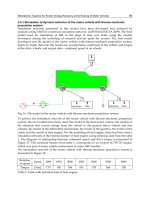
The concept of model-based friction compensation is depicted in Figure 1, where the friction
signal
ˆ
f
u is approximately equal to the actual plant friction
f
u , that is
ˆ
ff
uu ;
c
u is
control signal generated by the linear controller
c
G ;
in
u is actual input control signal into the
plant;
r
 is reference position signal;
out

is output position response of the system; 

is
velocity signal;

c
G is a linear controller designed with nominal plant model;
1
G is sub-
system model 1 and
2
G is sub-system model 2.
Though very simple, the effectiveness of the technique is anchored on the precision of the
friction model and the velocity estimation. It is implemented as either feedforward model-
based when the desired reference velocity is taken as the input to the model, or feedback
model-based when the input velocity is estimated from the sensed output. Both methods of
implementation have been adopted by different authors as reported by Armstrong (1994).

Advances in Mechatronics

46

Fig. 1. Block diagram of basic model-based friction compensation**
2.1 Parametric based friction models
Coulomb friction is the earliest physical model of friction based on the work of Da Vinci
(1519), Amontons (1699) and Coulomb (1785). It is described as a constant opposing force
independent of velocity of motion and is mathematically given by
s
g
n( )
fc
FF




(1)
and illustrated by Figure by Figure 2a
The viscous friction was developed by Reynold (1866) followed the birth of the theory of
hydrodynamics. Viscous friction is proportional to velocity, and it is zero when velocity
goes to zero

θ
f
FF




(2)
This led to the well known combine Coulomb plus viscous static model shown in Figure 2
(b), and represented by

θ
sgn( )
fc
FF F

 


(3)
This model has been widely applied in control system due to its simplicity. It has been
experimentally proven to be efficient for application above certain minimum velocity
(Armstrong, 1991). Canudas et al. (1986) employed Coulomb and viscous model in an
adaptive model-based friction compensation and has reported an improved performance in

terms of positioning accuracy. Based on its historical place in friction modeling, it is often
used for benchmarking the performance of other more complex models (Tjahjowidodo,
2004; Wahyudi and Tijani, 2008). The major problems with this model have been the failure
to account for friction at zero velocity and other several friction behaviors especially at low
velocity.
Morin (1833) introduced the idea of friction at rest known as stiction or static friction.
Stiction friction is defined as the force (torque) requires to initiate motion from rest, and is
generally greater than the Coulomb (Kinetic) friction. Friction was then seen to depend not
only on velocity but magnitude and rate of the external force. This resulted in a complete

Artificial Intelligent Based Friction Modelling and Compensation in Motion Control System

47
model of static friction as shown in Figure 2(c). However, Stribeck (1902) observed a
decreasing friction with increasing velocity at low velocity during the transition from
stiction to kinetic friction and he proposed the concept of Stribeck friction shown in Figure
2(d). In order to overcome the jump discontinuity of the model at zero velocity, a
modification was introduced (Karnopp, 1985) by replacing the jump with a line of finite
slope as shown in Figure 2(e). A combination of stiction, Stribeck, Coulomb and viscous
friction model is been referred to as Stribeck friction (Armstrong, 1991) or General Kinetic
Friction (GKF), (Evangelos et.al, 2002), and is described by

() () 0, 0
( ) 0, 0,
sgn( ) ( ) 0, 0,
f
fe es
se es
Ft
FFt FF

FFt FF








 


 


(4)
Several variant of Stribeck friction has been reported and evaluated by Armstrong (1991). A
general exponential form is given by

() ( )exp( sgn()
fcsc s
θ
FFFF F



  





(5)
where
f
F ,
s
F ,
c
F , and
θ
F

are the friction force, stiction, kinetic and viscous frictions
respectively,


is the velocity of motion,
s


is the Stribeck velocity, constant  is an
empirical parameter that determines the shape of the model, in which s
g
n( )


is defined as

1()0
s

g
n( ) 0 ( ) 0
1()0
t
t
t














(6)
where values of

=1 and

=2 indicate the Tustin /exponential model (1947) and Gaussian
model respectively.
Hess and Soom (1990) proposed another model of the form

2

() sgn()
1( )
sc
fc
θ
s
FF
FF F



 







(7)
which is known as Lorentzian friction model.
Tustin (1947) was the first to make use of a negative viscous friction (stribeck) in the analysis
of feedback control. Armstrong (1991) employed exponential, gaussian, Lorentzian together
with a polynomial model given by

2345678
234567
()
fc
θ

F FFFFFFFF

        

 
(8)
for friction identification in a robot arm system. The Lorentzian model gave best
performance fit and was later adopted for the friction compensation.
Several other researchers have employed the complete stribeck model both for fixed and
adaptive model-based friction compensation (Envangelos, et.al., 2002; and Lorinc and Bela,

Advances in Mechatronics

48
2007). Improved performance with respect to tracking and steady state accuracy have been
reported by them. A continuous, differentiable friction model with six parameters was
recently proposed by Makkar et al., (2005). The performance of the model was evaluated
with numbers of simulations and found to account for major friction effects such as
Coulomb, viscous, and stribeck. Its experimental implementation for friction compensation
has not yet been reported.


Fig. 2. Static friction models (a) Coulomb friction,(b) Coulomb + Viscous friction (c) Stiction
+ Coulomb + Viscous friction (d) Stiction + Stribeck + Coulomb + Viscous and (e) Modified
Stribeck friction (Karnopp Model)
Though the General Kinetic Friction (GKF) fails to account for pre-sliding friction behaviors
and other dynamics characteristics such as friction lag and local memory hysteresis,
experimental works have proven that a good static friction model can approximate the real
friction force with a degree of confidentiality of 90% (Armstrong, 1991; Lorinc and Bela,
2007). Also, Canudas de Wit et al., (1995) demonstrated that the simulated static friction

model and dynamic friction model predicts almost the same limit cycles generated by
friction in controlled positioning system. Hence, static friction model-based compensation
and identification techniques still have great significant practical applications.
Dynamic friction models have been proposed to account for various pre-sliding friction
behaviors and these are becoming essentials for higher precision performance at micro- and
nano- scale velocity and positioning control (Yi et. al., 2008). Some of the common dynamic
models which have been considered in control applications are Dahl, Lugre, Leuven, and
Generalized Maxwell-Slip (GMS). Dahl model (1968) was the first simple dynamic model
proposed for simulations of control system with friction. This was used for adaptive friction
compensation by Ehrich (1991) and is expressed as