Advances in Mechatronics Part 2 ppt

Integrated Control of Vehicle System Dynamics: Theory and Experiment

9
()( )()
zz
yxz f f r
xx
ab
mv v C C
vv


 


(30)

()()
zz
zz
ff
rzc
xx
ab
IaC bC M
vv

 



(31)
3. Investigation 1: Multivariable control
As mentioned earlier in the chapter, the first investigation addresses the coupling effects
between dynamics of the steering system and the suspension system. With this in mind, a
full-car dynamic model that integrates EPS and ASS is established. Then based on the
integrated model, a multivariable control method called stochastic sub-optimal control
strategy based on output feedback is applied to coordinate the control of both EPS and ASS.
3.1 State space formulation
For further analysis, it is convenient to formulate the full car dynamic model in state space
form by combining the dynamic models for the sub-systems that we developed earlier in
Section 2. Firstly, the state variables are defined as

12341234 1234
T
z uuuuuuuu ssgggg
X zzzzzzzz zzzzzz
  





 
 
(32)
and the output variables are chosen as











1 12 2 3 3 4 4 11 122 2 33 3 44 4
T
C z s u su s u s u s tg utg u tg u tg u
YT zzzzzzzzzkzzkzzkzzkzz


     



(33)
where
ui si
zz represents the suspension dynamic deflection at wheel i, and

ti
g
iui
kz z
represents the tyre dynamic load at wheel i. Therefore the state equation and output
equation can be written as

1223
() () () () ()

() ()
XtAXtBUtBUtBWt
Yt CXt

 






(34)
where
()Ut is the control input vector, and
1234
()[()()()()()]
T
m
Ut T t f t f t f t f t ;
2
()Ut
is the steering input vector, and

2
() ()
T
h
Ut t

 ; W(t) is the Gaussian white noise

disturbance input vector, and
1234
() [ () () () ()]
T
Wt w t w t w t w t .
3.2 Integrated controller design
The stochastic sub-optimal control strategy based on output feedback is applied to design
the integrated controller. This control strategy monitors the vehicle states and adjusts or
tunes the control forces for the ASS and the assist torque for the EPS by using the measured
outputs. The major advantage of the algorithm is that the critical parameters suggested by
the original dynamic system are automatically adjusted by the sub-optimal feedback law.
This overcomes the disadvantage resulted from that some of the state variables are
immeasurable in practice. To apply the control strategy, we first propose the objective
function (or performance indices) for the integrated control system defined in Eq. 34.

Advances in Mechatronics

10
Since it is a full-car dynamic model that integrates EPS and ASS, the multiple vehicle
performance indices must be considered, which include maneuverability, handling stability,
ride comfort, and safety. These performance indices can be measured by the following
physical terms: the torque applied on the steering wheel
c
T , the yaw rate of the full car
z

,
the pitch angle of sprung mass

, the roll angle of sprung mass


, the vertical acceleration
of sprung mass

s
z , the suspension dynamic deflection

s
u
zz, and the tyre dynamic load
()
t

ug
kz z . In addition, we also take into account the consumed control energy, which is
represented by the assist torque T
m
and the control force of the active suspension f
i.

Therefore, the integrated performance index is defined as

  










22
22 22
102345611
0
2
222
72 2 83 3 94 4 1011 1
222
2
11 2 2 2 12 3 3 3 13 4 4 4
2222
11 22 33 44
[
]
cz s us
us us us tgu
tg u tg u tg u mm
qT T q q qz q qz z
qzzqzzqzzqkzz
qkzz qkzz qkzz rT
rf rf rf rf dt
 





    










JE
(35)
where
113
,,qq , r
m
,
14
,rr are the weighting coefficients. We rewrite Eq. 35 in matrix form


00
00
0
TT TT T
TT
EYQYURUEXCQCXURU
EXQXURU




 


 

 


 








dt dt
dt
J
(36)
where
T
0
QCQC ;


0
 
12 13

diag q ,q , ,qQ
;


m1234
,,,,R  diag r r r r r
.
To minimize the above performance index, the sub-optimal feedback control law is
developed as follows.
The control matrix
U can be expressed by

U-KY
(37)
where
K is the output feedback gain matrix, which can be derived through the following
procedure.
Step 1. We first can derive the state feedback gain matrix F

using optimal control method:

1 T
FRBP

 (38)
where the matrix
B is calculated as
1
11
BAAB


 ; and the matrix P is the solution of the
following
Riccati equation:

1
0
TT
PA A P PBR B P Q


 (39)
Step 2. Since there is no inverse matrix for the non-square (or rectangular) matrix C, the
output feedback gain matrix
K cannot be directly obtained through the equation KC F

 . In

Integrated Control of Vehicle System Dynamics: Theory and Experiment

11
this case, the norm-minimizing method is used to find the approximate solution of K (Gu et
al., 1997). First, the following objective function is constructed


2
22 22
*
11
ij ij

ij
HFF FF


  

(40)
and then we can find F by minimizing the objective function H



1
TT
FFCCC C


 (41)
we also have

FKC

(42)
Thus
K is derived by combining Eq. 41 and Eq. 42



1
TT
KFCCC



 (43)
and the control matrix
U becomes



1
TT
UKYFCCC Y


 
(44)
3.3 Simulations and discussions
The integrated control system is analyzed using Matlab/Simulink. We assume that the
vehicle travels at a constant speed
v
x
= 20m/s, and is subject to a steering input from
steering wheel. The steering input is set as a step signal with amplitude of 120º.
The road excitation shown in Fig. 4 is assumed to be independent for each wheel and the
power of the white noise for each wheel equals 20dB. The assumption of independent road
excitation for each wheel has practical significance because in real road conditions, the road
excitations on the four wheels of the vehicle are different and independent. It must be noted
that this assumption on the road excitation is different from the assumption commonly
made in other studies. The commonly made assumption states that the rear wheels follow
the front wheels on the same track and hence the excitations at the rear wheels are just the
same as the front wheels except for a time lag. Such a simplification is not applied in this

simulation. The values of the vehicle physical parameters used in the simulation are listed in
Table 1.
The parameter setting for the weighting coefficient matrices
Q
0
and R defined in Eq. 36
plays an important role in the simulation performance. After tuning these weighting
coefficients, we choose the following parameter setting when a satisfactory system
performance is achieved:
1
10q

,
6
2
10q 
,
5
3
5.0 10q 
,
6
45
210qq
,
3
67 13
10qq q 
,
0.1

m
r

, and
1234
1rrrr

.
It must be noted that different levels of importance are assigned to the different
performance indices with such a parameter setting for the weighting coefficients. For
example, the vertical acceleration of sprung mass is considered to be more important than
the suspension dynamic deflection. In order to study comprehensively the characteristics of


Advances in Mechatronics

12
N
2
20 c
3
/c
4

1760/ 1760 (N
s/m)
k
s

90 (N

m/ rad)
k
t
138000 (N/m)
I
p

0.06 (kg
m
2
)
h
0.505 (m)
c
e

0.3 (N
sm/rad)
d
0.64 (m)
M
1030 (kg)
a
0.968 (m)
m
s
810 (kg)
b
1.392 (m)
m

u1
/m
u2
26.5/ 26.5 (kg) I
x

300 (kg
m
2
)
m
u3
/m
u4
24.4/ 24.4 (kg) I
y

1058.4 (kg
m
2
)
k
s1
/k
s2
20600/ 20600 (N/m) I
z

1087.8 (kg
m

2
)
k
s3
/k
s4
15200/ 15200 (N/m) f
0
0.01 (Hz)
k
af
/k
ar

6695/ 6695 (N
m/ rad)
G
0
5.0×10
-6
(m
3
/cycle)
c
1
/c
2

1570/ 1570 (N
s/m)

v
x

20m/s
Table 1. Vehicle Physical Parameters.
the integrated control system, the integrated control system is compared to two other
systems. One is the system without control, i.e. the passive mechanical system. While
the other is the system that only has ASS (denoted as ASS-only) or EPS (denoted as EPS-
only). For each of the two control systems, the sub-optimal control strategy is applied
and the identical parameter setting for the weighting coefficient matrices
Q
0
and R is
selected.
It can be observed from the simulation results that all the performance indices are improved
for the integrated control system, compared to those for the passive system, and those for
ASS-only or EPS-only. For brevity, only the performance indices with higher lever of
importance are selected to illustrate in Fig. 5 through Fig. 8. The following discussions are
made:

1. As shown in Fig. 5, the roll angle for the integrated control system is reduced
significantly compared to that for the ASS-only system and the passive system. A
quantitative analysis of the results shows that the peak value of the roll angle for the
integrated control system is decreased by 37.6%, compared to that for the ASS-only
system, and 55.3% for the passive system. Moreover, the roll angle for the integrated
control is damped quickly and thus less oscillation is observed for the integrated control
system, compared to the other two systems. Therefore the results indicate that the anti-
roll ability of the vehicle is greatly enhanced and thus a better handling stability is
achieved through the application of the integrated control system.
2.

It is presented clearly in Fig. 6 that the overshoot of the yaw rate for the integrated
control system is decreased compared to that for the EPS-only system and the passive
system. Furthermore, the yaw rate for the integrated control system and the EPS-only
system becomes stable more quickly than the passive system after the overshoot.
However, there is no significant time difference for the integrated control system and
the EPS-only system to stabilize the yaw rate after the overshoot. The results
demonstrate that the application of the integrated control system contributes a better
lateral stability to the vehicle, compared to the EPS-only system and the passive system.
3.
A quantitative analysis is performed for the vertical acceleration of sprung mass as
shown in Fig. 7. The obtained R.M.S. (Root-Mean-Square) value of the vertical
acceleration of sprung mass for the integrated control system is reduced by 23.1%,

Integrated Control of Vehicle System Dynamics: Theory and Experiment

13
compared to that for the ASS-only system, and 35.5% for the passive system. The results
show that the vehicle equipped with the integrated control system has a better ride
comfort than that with the ASS-only system and the passive system. In addition, the
dynamic deflection of the front suspension as shown in Fig. 8 also suggests similar
results.
In summary, the integrated control system improves the overall vehicle performance
including handling, lateral stability, and ride comfort, compared to either the EPS-only
system or the ASS-only system, and the passive system.


Fig. 4. Road Input.


Fig. 5. Roll angle.

1. Passive
2. ASS-only
3. Integrated Control

Advances in Mechatronics

14




Fig. 6. Yaw rate.





Fig. 7. Vertical acceleration of sprung mass.
1. Passive
2. EPS-only
3. Integrated Control
1. Passive
2. ASS-only
3. Integrated Control

Integrated Control of Vehicle System Dynamics: Theory and Experiment

15

(a) (b)

Fig. 8. Front suspension deflection: (a) at wheel 1; (b) at wheel 2.
In this investigation, a full-car dynamic model has been established through integrating
electrical power steering system (EPS) with active suspension system (ASS) in order to
address the coupling effects between the dynamics of the steering system and the
suspension system. Thereafter, a multivariable control approach called stochastic sub-
optimal control strategy based on output feedback has been applied to coordinate the
control of both the EPS and ASS. Simulation results show that the integrated control system
is effective in fulfilling the integrated control of the EPS and the ASS. This is demonstrated
by the significant improvement on the overall vehicle performance including handling,
lateral stability, and ride comfort, compared to either the EPS-only system or the ASS-only
system, and the passive system. However, the development of the integrated vehicle control
system requires fully understanding the vehicle dynamics in both the global level and
system or subsystem level. Thus the development task for the integrated vehicle control
system becomes very difficulty when the number of control systems increases. Furthermore,
a whole new design is required for the integrated vehicle control system including both
control logic and hardware, when a new control system, e.g. anti-lock brake system (ABS), is
equipped with.
4. Investigation 2: Hierarchical control
In the above investigation, we demonstrated the effectiveness of one of the integrated
control approaches called multivariable control on coordinating the control of the ASS and
the EPS. While the second investigation moves up a step further on developing the
integrated control approach. To this end, a hierarchical control architecture is proposed for
integrated control of active suspension system (ASS) and electronic stability program (ESP).
The advantages of the hierarchical control architecture are demonstrated through the
following design practice of the integrated control system.
4.1 Hierarchical controller design
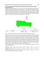
The architecture of the proposed hierarchical control system is shown in Fig. 9. The control
system consists of two layers. The upper layer controller monitors the driver’s intentions
1. Passive
2. ASS-only

3. Integrated Control
1. Passive
2. ASS-only
3. Integrated

Advances in Mechatronics

16
and the current vehicle states including the steering angle of the front wheel
f

, the sideslip
angle

, the yaw rate
z

and the lateral acceleration
y
a , etc. Based on these input signals,
the upper layer controller computes the corrective yaw moment
zc
M
in order to track the
desired vehicle motions. Thereafter, the upper layer controller generates the distributed
torques
ESP
M and
A
SS

M to the two lower layer controllers, i.e., the ESP and the ASS,
respectively, according to a rule-based control strategy. Moreover, the distributed torques
ESP
M and
A
SS
M are converted into the corresponding control commands for the two
individual lower layer controllers. Finally, the ESP and the ASS execute respectively their
local control objectives to control the vehicle dynamics. The upper layer controller and the
two lower layer controllers are designed as follows.

x
v
ASS
M
ESP
M
s
z

y
a
z

z

ˆ

z


ˆ

ˆ

z

x
v
s
z

y
a
f

w

w
p

Fig. 9. Block diagram of the hierarchical control system.
4.2 Upper layer controller design
It is known that both the applications of the ESP and the ASS are able to develop corrective
yaw moments (either directly or indirectly). To coordinate the interactions between the ASS
and the ESP, a simple rule-based control strategy is proposed to design the upper layer
controller. The aim of the proposed control rule is to distribute the corrective yaw moment
appropriately between the two lower layer controllers. The control rule is described as
follows.
First, the corrective yaw moment
zc

M
is calculated by using the 2-DOF vehicle reference
model defined in Section 2.5, based on the measured and estimated vehicle input signals.
Second, the braking/traction torque
d
M
and the pitch torque
p
M
are computed by using
the following equations

0.5
d
p
wzcww
MMI


 

cp
(45)

α
λ
α
=
p
d

w
ktan
M
M
c

(46)
where Eq. (45) is derived by considering the dynamics of one of the front wheels. It should
be noted that although a front wheel drive vehicle is assumed, the main conclusions of this

Integrated Control of Vehicle System Dynamics: Theory and Experiment

17
study can be easily extended to vehicles with other driveline configurations; In general, the
brake torque at each wheel is a function of the brake pressure
w
p
at that wheel, and
p
c is
an equivalent braking coefficient of the braking system, which is determined by using the
equation
p
wbb
cAR

 ; The number “0.5” represents that the corrective yaw moment is
evenly shared by the two front wheels.
Finally, the distributed torques
ESP

M and
ASS
M are generated by using a linear
combination of the braking/traction torque
d
M
and the pitch torque
p
M
, which is given as

11
22
(1 - )
(1 - )
ESP d
p
A
SS
p
d
M
nM n M
M
nM n M








(47)
where
1
n and
2
n are the weighting coefficients, and
1
10.5n ,
2
10.5n . Therefore,
through tuning the weighting coefficients
1
n and
2
n , the upper layer controller is able to
coordinate the two lower layer controllers and determine to what extent the two lower layer
controllers to be controlled.
4.3 Lower layer controller design
4.3.1 ASS controller design
The LQG control method is used to control the active suspension system. The state variables
are defined as
[
s
Xz


s
z



1u
z
2u
z
3u
z
4u
z
1u
z


2u
z


3u
z


4u
z

θ







]
T
; and the output
variables are chosen as
Y =[
s
z


1u
z
2u
z
3u
z
4u
z θ

]
T
. Therefore, based on Eq. 4 through
Eq. 16, together with the road excitation model presented in Section 2.4, the state equation
and the output equation can be written as


XAXBU
YCXDU









(48)
where
U  [
1
U
2
U ]
T
is the control input vector.
1
U =[
1
f

2
f

3
f

4
f

]
T
is the control force
vector, and
2
U =[
1
g
z
2
g
z
3
g
z
4
g
z ]
T
is the road excitation vector. The multiple vehicle
performance indices are considered to evaluate the vehicle handling stability, ride comfort,
and safety. These performance indices can be measured by the following physical terms:
vertical displacement of each wheel
1u
z ,
2u
z ,
3u
z ,
4u

z ; the suspension dynamic deflections
11
()
su
zz ,
22
()
su
zz ,
33
()
su
zz ,
44
()
su
zz ；the vertical acceleration of sprung mass
s
z

;
the pitch angular acceleration


; the roll angular acceleration


; and the control forces of
the active suspension
1

f
,
2
f
,
3
f
,
4
f
. Therefore, the combined performance index is defined
as

2222 2
11 22 33 44 5 1 1
0
2222
6227338449
2 22222
10 11 1 1 2 2 3 3 4 4
1
[()
()()()
]
T
uuuu su
T
su su su
s
J Lim qz qz qz qz q z z

T
qzzqzzqzzq
qqzrfrfrfrfdt





 




(49)

Advances in Mechatronics

18
where
1
q ,…,
11
q , and
1
r ,…,
4
r are the weighting coefficients. The above equation can be
rewritten as the following matrix form



J
0
1
(2)
T
TT T
T
Lim X QX U RU X NU dt
T



(50)
where Q ,
R , N are the weighting matrices.
The state feedback gain matrix K is derived using the optimal control method, and it is the
solution of the following Riccati equation

1
11 222
0
TTT
KA A K Q KB R B K B U B


   (51)
4.3.2 ESP controller design
In this study, an adaptive fuzzy logic (AFL) method is applied to the design of the ESP
controller. Fuzzy logic controller (FLC) has been identified as an attractive control method
in vehicle dynamics control (Boada et al., 2005). This method has advantages when the

following situations are encountered: 1) there is no explicit mathematical model that
describes how control outputs functionally depend on control inputs; 2) there are experts
who are able to incorporate their knowledge into the control decision-making process.
However, traditional FLC with a fixed parameter setting cannot adapt to changes in the
vehicle operating conditions or in the environment. Therefore, an adaptive mechanism must
be introduced to adjust the controller parameters in order to achieve a satisfactory vehicle
performance in a wide range of changing conditions.

,
f
v

z

z
e



,ede
z
c
M
ˆ


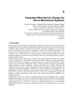
Fig. 10. Block diagram of the adaptive fuzzy logic controller for ESP.
As shown in Fig. 10, the AFL controller consists of a FLC and an adaptive mechanism. To
design the AFL controller, the yaw rate and the sideslip angle of the vehicle are selected as
the control objectives. The yaw rate can be measured by a gyroscope, but the sideslip angle

cannot be directly measured and thus has to be estimated by an observer. The observer is
designed by using the 2-DOF vehicle model described in Section 2.4. The linearized state
space equation of the 2-DOF vehicle model is derived as follows, with the assumptions of a
constant forward speed and a small sideslip angle.

EE
EE
XAXBU
YCXDU


 



 



(52)

Integrated Control of Vehicle System Dynamics: Theory and Experiment

19
where
z
X







,
f
zc
U
M








,
2
22
1
fr f r
fr f r
zz
CC aCbC
mv
mv
E
aC bC a C b C
IIv
A
















,
1
0
f
f
zz
C
mv
E
aC
II
B












,
10
01
E
C




,
00
00
E
D







.

The aim of the AFL is to track both the desired yaw rate and the desired sideslip angle. The
desired yaw rate is calculated as

2
(1 )
xf
ze
x
v
LSv





(53)
where
L
is the wheel base; S is the stability factor of the vehicle, and
2
(/ / )/
fr
SmbC aC L . As shown in Fig. 10, the FLC has two input variables, the tracking
error of the yaw rate
e and the difference of the error de . They are defined as, at the kth
sampling time

() () ()
zze
ek k k


 (54)

() () ( 1)de k e k e k

 (55)
The output variable of the FLC is defined as the corrective yaw moment
zc
M
. To determine
the fuzzy controller output for the given error and its difference, the decision matrix of the
linguistic control rules is designed and presented in Table 2. These rules are determined
based on expert knowledge and a large number of simulation results performed in the
study. In designing the FLC, the scaling factors
e
k and
de
k have great effects on the
performance of the controller. Therefore the adaptive mechanism is applied to adjust the
parameters in order to achieve a satisfactory control performance when there are changes in
the vehicle operating conditions or in the environment. The adaptive law is given as

0
0
() ( )
t
y
eez
a
kk dt

v
 
 

(56)

1
() ( )
de z de y x
kkaasin
v


  

cos
(57)
where
0
0


. Full details of the derivation of the above equations are given in the
Appendix.
4.4 Simulations and discussions
In order to evaluate the performance of the developed hierarchical control system, a
simulation investigation is performed. The performance and dynamic behaviors of the
hierarchical control system are analyzed using Matlab/Simulink. We assume that the
vehicle travels at a constant speed
v

= 90 km/h. Two driving conditions are performed: 1)
step steering input; and 2) double lane change. For the first case, the vehicle is subject to a


Advances in Mechatronics

20
de
e
PB PM PS O NS NM NB
PB NB NB NB NB NM O O
PM NB NB NB NB NM O O
PS NM NM NM NM O PS PS
PO NM NM NS O PS PM PM
NO NM NM NS O PS PM PM
NS NS NS O PM PM PM PM
NM O O PM PB PB PB PB
NB O O PM PB PB PB PB
Table 2. Fuzzy rule bases for ESP control.
steering input from the steering wheel and the steering input is set as a step signal with
amplitude of 120º. The road excitation is assumed to be independent for the four wheels.
After tuning the parameter setting for the hierarchical control system, we select the
weighting parameters for the ASS:
1234
1rrrr

,
3
1234
10qqqq ,

4
5678
10qqqq ,
3
9
210q  ,
5
10
10q  , and
6
11
10q  . Moreover, the weighting
parameters for the upper layer controller are selected as:
1
0.80n

and
2
0.85n

.
The simulation results for the multiple performance indices are shown in Fig. 11 and Fig. 12
(For brevity, only some representative performance indices are presented here).

012345
-1
0
1
2
3

4
5
6
7
8
Hierarchical control
Non-integrated control
Sideslip angle (deg)
Time (s)

12345
-0.05
0.00
0.05
0.10
0.15
0.20
0.25
0.30
Hierarchical control
Non-integrated control
Yaw rate (rad/s)
Time (s)

(a) (b)

012345
-6
-4
-2

0
2
4
6
8
10
12
Hierarchical control
Non-integrated control
Lateral acceleration (m/s
2
)
Time (s)

012345
-5
-4
-3
-2
-1
0
1
2
3
4
5
6
7
8
9

10
Hierarchical control
Non-integrated control
Vertical Acceleration (m/s
2
)
Time (s)

(c) (d)
Fig. 11. Comparison of responses for the manoeuvre of step steering input: (a) sideslip angle;
(b) yaw rate; (c) lateral acceleration; (d) vertical acceleration.

Integrated Control of Vehicle System Dynamics: Theory and Experiment

21
012345678
-6
-5
-4
-3
-2
-1
0
1
2
3
4
5
6
7

Hierarchical control
Non-integrated control
Sideslip angle (deg)
Time(s)

012345678
-0.25
-0.20
-0.15
-0.10
-0.05
0.00
0.05
0.10
0.15
0.20
0.25
Hierarchical control
Non-integrated control
Yaw rate (rad/s)
Time (s)

(a) (b)
012345678
-6
-5
-4
-3
-2
-1

0
1
2
3
4
5
6
Hierarchical control
Non-integrated control
Lateral Acceleration (m/s
2
)
Time (s)

012345678
-3
-2
-1
0
1
2
3
4
Hierarchical control
Non-integrated control
Vertical acceleration (m/s
2
)
Time (s)

(c) (d)
Fig. 12. Comparison of responses for the manoeuvre of double lane change: (a) sideslip
angle; (b) yaw rate; (c) lateral acceleration; (d) vertical acceleration.
For comparisons, the simulation investigation for non-integrated control is also performed.
In the case, we simply eliminate the upper layer controller. The following discussions are
made:
1.
For the manoeuvre of step steering input, it can be seen that the peak value of the
sideslip angle for hierarchical control, as shown in Fig. 11(a), is reduced by 11.6%
compared to that for non-integrated control. Moreover, the sideslip angle for
hierarchical control is damped quickly and thus has less oscillation than that for non-
integrated control. Similar patterns can be observed for the yaw rate and the lateral
acceleration illustrated in Fig. 11(b) and Fig. 11(c), respectively. The results indicate that
the vehicle lateral stability is improved by the proposed hierarchical control system in
comparison with the non-integrated control system. In addition, the vertical
acceleration of sprung mass, one of ride comfort indices, is presented in Fig. 11(d). It
can be observed that the peak value of the performance index is decreased by 13.8% for
hierarchical control, compared to that for non-integrated control.

Advances in Mechatronics

22
2. For the manoeuvre of double lane change, it is observed that the peak value of the
sideslip angle for hierarchical control is reduced by 15.3% compared to that for non-
integrated control, as shown in Fig. 12(a). Moreover, for the peak value of the yaw rate
shown in Fig. 12(b), the percentage of decrease is 7.9. However, as shown in Fig. 12(c),
there is no significant difference on the lateral acceleration between the two control
cases. While for the vertical acceleration of sprung mass shown in Fig. 12(d), it can be
seen clearly that the peak value of this performance index for hierarchical control is
reduced significantly by 30.5%, compared to that for non-integrated control. In

addition, a quantitative analysis of the vertical acceleration shows that the R.M.S. (Root-
Mean-Square) value of the vertical acceleration for hierarchical control is reduced by
21.9% compared to that for non-integrated control.
In summary, the application of the hierarchical control system improves the overall vehicle
performance including the ride comfort and the lateral stability under the critical driving
conditions. The results show that the hierarchical control system is able to coordinate the
interactions between the ASS and the ESP and thus expand the functionalities of the two
individual control systems.
5. Investigation 3: Experiment
To verify the effectiveness of the proposed hierarchical control architecture, an experimental
study is performed. A physical configuration of the two-layer hierarchical control
architecture is illustrated in Fig. 13. The upper layer controller determines the corrective
yaw moment to track the desired vehicle motions by using the signals from the CAN-bus,
e.g. driver’s intentions, environment information, and current vehicle dynamic states.
Thereafter, the upper layer controller generates the distributed torques to the two lower
layer controllers, i.e., the ESP and the ASS, respectively, according to a rule-based control
strategy. Moreover, the distributed torques are converted into the corresponding control
commands for the two individual actuators to regulate or track respectively the vehicle
dynamic states.
Development and test of complex control systems often benefit from a technique called
hardware-in-the-loop (HIL) simulation. The advantages of this technique over real plant
tests include: greater flexibility and higher safety in the test scenarios, shorter development
time and reduced cost, and measurable/reproducible criteria for system and subsystem
evaluation. With those in mind, the HIL simulation is applied to verify the effectiveness of
the proposed hierarchical control system. Fig. 14 shows the developed hardware-in-the-loop
test platform for the hierarchical control system. The client computer (PXI-8196 by National
Instruments Inc.) collects the signals measured by the sensors, which include the pressure of
each brake wheel cylinder, the pressure of brake master cylinder, and the vertical
acceleration of sprung mass at each suspension, etc. These signals are in turn provided to
the host computer (PC) through CAN-bus. Based on these input signals, the host computer

computes the vehicle states and the desired vehicle motions, such as the desired yaw rate.
Thereafter, the host computer generates control commands to the client computer. Through
the hardware interface circuits, the client computer in turn sends the control commands to
the corresponding actuators.
The experimental setup is shown in Fig. 15. A test vehicle was equipped with the developed
control units for the upper layer controller, ESP controller and ASS controller. The test
vehicle was running on a road simulator, which is mounted on the test ground as shown in

Integrated Control of Vehicle System Dynamics: Theory and Experiment

23
the figure. Therefore the road excitation signal can be generated through the road simulator.
Again, the two same driving conditions as those used in the simulation investigation were
performed, i.e., the manoeuvre of step steering input and the manoeuvre of double lane
change. Two cases were tested in the experiment, one is “with hierarchical control”, and the
other is “non-integrated control”. For both testing cases, numerous vehicle tests were
performed to validate the developed control units. The measured dynamic responses of the
vehicle performance indices are illustrated in Fig. 16 for the manoeuvre of step steering
input and Fig. 17 for the manoeuvre of double lane change, respectively.



Fig. 13. Physical configuration of the hierarchical control architecture.



Fig. 14. HIL experimental configuration.

Advances in Mechatronics

24

Fig. 15. Experimental setup.

012345
-1
0
1
2
3
4
5
6
7
8
9
10
11
Hierarchical control
Non-integrated control
Sideslip angle (deg)
Time (s)

12345
-0.05
0.00
0.05
0.10
0.15
0.20

0.25
0.30
Hierarchical control
Non-integrated control
Yaw rate (rad/s)
Time (s)

(a) (b)

012345
-6
-4
-2
0
2
4
6
8
10
12
Hierarchical control
Non-integrated control
Lateral acceleration (m/s
2
)
Time (s)

012345
-5
-4

-3
-2
-1
0
1
2
3
4
5
6
7
8
Hierarchical control
Non-integrated control
Vertical Acceleration (m/s
2
)
Time (s)

(c) (d)

Fig. 16. Comparison of responses for the manoeuvre of step steering input: (a) sideslip angle;
(b) yaw rate; (c) lateral acceleration; (d) vertical acceleration.

Integrated Control of Vehicle System Dynamics: Theory and Experiment

25
012345678
-8
-7

-6
-5
-4
-3
-2
-1
0
1
2
3
4
5
6
7
8
Hierarchical control
Non-integrated control
Sideslip angle (deg)
Time(s)

012345678
-0.25
-0.20
-0.15
-0.10
-0.05
0.00
0.05
0.10
0.15

0.20
0.25
Hierarchical control
Non-integrated control
Yaw rate (rad/s)
Time (s)

(a) (b)
012345678
-6
-5
-4
-3
-2
-1
0
1
2
3
4
5
6
Hierarchical control
Non-integrated control
Lateral Acceleration (m/s
2
)
Time (s)

012345678

-4
-3
-2
-1
0
1
2
3
Hierarchical control
Non-integrated control
Vertical acceleration (m/s
2
)
Time (s)

(c) (d)
Fig. 17. Comparison of responses for the manoeuvre of double lane change: (a) sideslip
angle; (b) yaw rate; (c) lateral acceleration; (d) vertical acceleration.
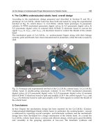
The following discussions are made by comparing the corresponding performance indices
for hierarchical control and non-integrated control:
1.
For the manoeuvre of step steering input, it is shown clearly in Fig. 16(a) that the peak
value of the sideslip angle for hierarchical control is reduced by 25.1%, compared to
that for non-integrated control. The similar phenomena can be observed in Fig. 16(b) for
the yaw rate and Fig. 16(c) for the lateral acceleration, except that the percentages of
decrease for the two performance indices are slightly smaller than that for the sideslip
angle. In addition, as shown in Fig. 16(d), the peak value of the vertical acceleration of
sprung mass is decreased greatly by 30.1% for hierarchical control, compared to that for
non-integrated control. The results indicate that both the lateral stability and the ride
comfort are improved by the proposed hierarchical control system in comparison with

the non-integrated control system.
2.
For the manoeuvre of double lane change, it is observed in Fig. 17(a) through Fig. 17(c)
that the peak values of the sideslip angle, the yaw rate, and the lateral acceleration have

Advances in Mechatronics

26
certain amount of decrease for hierarchical control, compared to those for non-
integrated control. Moreover, a smaller R.M.S. value can be observed for those
performance indices even without calculation. Finally, as presented in Fig. 17(d), the
peak value of the vertical acceleration of sprung mass for hierarchical control is reduced
significantly by 59.2%, compared to that for non-integrated control. A quantitative
analysis of the vertical acceleration shows that the R.M.S. value of the vertical
acceleration for hierarchical control is reduced by 47.9% compared to that for non-
integrated control.
3.
The experimental results have good agreement with the simulation results on
demonstrating the vehicle performance improvements by the proposed hierarchical
control system.
In summary, the experimental results demonstrate that the proposed hierarchical control
system is able to improve both the lateral stability and the ride comfort, in comparison with
the non-integrated control system. The experimental results verify the effectiveness of the
hierarchical control system.
In the second and third investigations, integrated control and coordination of active
suspension system (ASS) and electronic stability program (ESP) have been studied by using
hierarchical control strategy. A two-layer hierarchical control architecture has been
proposed to achieve the goal of function integration for the two chassis control systems. The
upper layer controller has been designed to coordinate the interactions between the ASS and
the ESP. A rule-based control method has been used to design the upper layer controller. In

addition, the two lower layer controllers including the ASS and the ESP, have been designed
independently to achieve their local control objectives. The LQG control strategy and the
adaptive fuzzy logic control method have been used to design the ASS and the ESP,
respectively. Both a simulation investigation and a hardware-in-the-loop experimental
study have been performed. Simulation results demonstrate that the proposed hierarchical
control system is able to improve the multiple vehicle performance indices including both
the ride comfort and the lateral stability. Moreover, the experimental results verify the
effectiveness of the design of the hierarchical control system.

6. Conclusions
In this chapter, integrated control and coordination of vehicle system dynamics have been
studied comprehensively and intensively through theoretical developments and
experimental verifications. The study consists of three investigations. The first investigation
has been focused on coordinating the interactions and function conflicts between the
steering system and the suspension system by using a multivariable control approach called
stochastic sub-optimal control strategy. Simulation results show that the integrated control
system is effective in improving the overall vehicle performance including handling, lateral
stability, and ride comfort, compared to either the EPS-only system or the ASS-only system,
and the passive system. Moreover, a more advanced integrated control approach called
hierarchical control method has been applied to coordinate control of the ASS and the ESP.
The design flexibility of the hierarchical control method has been demonstrated through the
design practice of the two-layer control system. The upper layer controller has been
designed to coordinate specifically the interactions between the ASS and the ESP. While the
two lower layer controllers including the ASS and the ESP, have been designed
independently to achieve their local control objectives. The application of the hierarchical
control method to upper layer controller design has been focused on function coordination

Integrated Control of Vehicle System Dynamics: Theory and Experiment

27

of the two lower layer control systems and thus few modifications are required for the two
subsystems, in contrast to the multivariable control approach. Finally, both a simulation
investigation and a hardware-in-the-loop experimental study have been performed.
Simulation and experimental results demonstrate that the proposed hierarchical control
system is able to improve the multiple vehicle performance indices including both the ride
comfort and the lateral stability, compared to the non-integrated control system.
7. Acknowledgement
This research was sponsored in part by the Natural Science Foundation of China under
Grant No. 51075112, and the Royal Society of UK under Grant No. 16558.
8. Nomenclature
a, b: horizontal distance between the C.G. of the vehicle and the front, rear axle;
A, B: state matrix, input matrix;
w
A : brake area of the wheel;
c
e
: equivalent damping coefficient reflected to the pinion axis;
c
i
: damping coefficient of the suspension at wheel i;
c
p
: equivalent braking coefficient of the braking system;
c

: lateral stiffness of the tyre;
C: output matrix;
C
f
, C

r
: corning stiffnesses of the front tyre and the rear tyre, respectively;
d: half of the wheel track;
de: difference of the yaw rate tracking error;
D: feedforward matrix;
e: yaw rate tracking error;
f
0
: low cut-off frequency;
f
1
~ f
4
: control force of each active suspension controller;
f
r
: rolling resistance coefficient;
F
x1
~ F
x4
and F
y1
~ F
y4
: longitudinal and lateral forces of the four wheels, respectively;
F
z1
~ F
z4

: total force of the suspension acting on the sprung mass;
G
0
: road roughness coefficient;
h: vertical distance between the C.G. of sprung mass and the roll center;
I
p
: equivalent moment of inertia of multiple parts reflected to the pinion axis. The multiple
parts include the motor, the gear assist mechanism, and the pinion;
I
w
: wheel moment of inertia about its spin axis;
I
x
, I
y
, I
z
: roll moment of inertia, pitch moment of inertia, and yaw moment of inertia of
sprung mass;
I
xz
: product of inertia of sprung mass about the roll and yaw axes;
J: performance index;
k
af
, k
ar
: stiffness of the anti-roll bars for the front, rear suspension;
k

e
, k
de
: scaling factor;
k
s
: torsional stiffness of the torque sensor;
k
si
: stiffness of the suspension at wheel i;
k
ti
: stiffness of tyre at wheel i;

Advances in Mechatronics

28
k

: cornering stiffness of the tyre;
K: state feedback gain matrix;
L: wheel base;
m, m
s
, m
ui
: mass of the vehicle, sprung mass, and unsprung mass at wheel i;
M
ASS
, M

ESP
: distributed torques for the ASS and the ESP, respectively;
M
d
, M
p
: braking/traction torque and pitch torque;
M
ZC
: corrective yaw moment generated by the ESP controller;
n
1
, n
2
: weighting coefficient;
N: weighting matrix;
N
2
: speed reduction ratio of the rack-pinion mechanism;
w
p
: pressure of the brake wheel cylinder;
q
1
,…, q
11
, r
1
,…, r
4

: weighting coefficient;
Q, R: weighting matrix;
R
b
: brake radius;
R
w
: tyre rolling radius;
S: vehicle stability factor;
T
0
: ideal steering torque applied on the steering wheel;
T
c
: torque applied on the steering wheel;
T
i
: wheel torque at wheel i;
T
m
: assist torque applied on the steering column;
T
r
: aligning torque transferred from tyres to the pinion;
T
zwi
: aligning torque acting on the tyre i;
U, U
1
, U

2
: control input vector, control force vector, and road excitation vector, respectively;.
v, v
x
, and v
y
: vehicle speed, vehicle speed in the longitudinal direction and the lateral
direction, respectively;
w
i
: zero-mean Gaussian white noise with intensity of 1;
X, Y: state vector, output vector;
z
gi
: road excitation;
z
s
: vertical displacement of sprung mass;
z
ui
: vertical displacement of unsprung mass;

: sideslip angle of the tyre;

: sideslip angle of the vehicle at the C.G.;
1

: rotation angle of the pinion;
f


,
r

: steering angles of the front, rear wheels;
i

: steering angle of wheel i;

: roll angle of sprung mass;
w

: pneumatic trail of the tyre;
b

: brake friction coefficient;

: pitch angle of sprung mass;
h

: rotation angle of the steering wheel;
i

: angular velocity of wheel i;
z

,
ze

: yaw rate of the vehicle, desired yaw rate of the vehicle;