Advances in Mechatronics Part 11 potx

Recognition of Finger Motions for Myoelectric Prosthetic Hand via Surface EMG

189
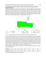
From Fig.14, the recognition of the finger motion was performed correctly.
The operation of the robot hand is determined as follows. In both thumb and index finger,
extension is in the state where the finger is lengthened, and flexion is in the state where the
finger is bent at 90 degrees. In control of the thumb, the reference value for the flexion was
set as 0.95 rad, which is the rotation angle of the pulley required to make the thumb bent at
90 degrees. On the other hand, the reference value for the extension was set as 0 rad in order
to return the thumb to the original state. Likewise, in control of the index finger, the
reference value for the flexion was set as 2.86 rad, which is the rotation angle of the pulley
required to make the index finger bent at 90 degrees. On the other hand, the reference value
for the extension was set as 0 rad in order to return the index finger to the original state. PI
controllers were adopted in the construction of the servo systems, and the controller gains of
the PI controllers were adjusted by trial and error through repetition of the experiments. The
result of the operation of the robot hand is shown in Fig.15, in which the blue dashed line
shows the reference value of the rotation angle of the pulley, and the red solid line shows
the rotation angle of the actual pulley driven by motor.
The result shown in Fig.15 is the case where the recognition results of the finger motion for
both the thumb and the index finger were successful, and both the thumb and the index
finger of the robot hand were able to be operated as intended.
6. Conclusion
In this chapter, a robot hand for myoelectric prosthetic hand, which has thumb and index
finger and can realize "fit grasp motion", was proposed and built. In order to control each
finger of the developed myoelectric prosthetic hand independently, recognition of four
finger motions, namely flexion and extension of the thumb and of the index finger in MP
joint, was performed based on the SEMG using the neural network(s). First, recognition of
these four finger motions by one neural network was executed. Then, the successful
recognition rate was only 20.8% on average. In order to improve the recognition rate, three
types of the improved identification methods were proposed. Simulation results for the

recognition rate using each improved identification method showed successful recognition
rate of more than 57.5% on average. Experiment for online recognition of the finger motions
was carried out using the identification method which showed the most successful
recognition rate, and similar recognition result as in the simulation was obtained.
Experiment for online finger operation of the robot hand was also executed. In the
experiment, the fingers of the robot hand were controlled online based on the recognition
result by the identifier via SEMG, and both the thumb and the index finger of the robot hand
were able to be operated as intended.
7. Acknowledgement
The author thanks Dr. T. Nakakuki for his valuable advices on this research, and thanks Mr.
A. Harada for his assistance in experimental works.
8. References
Farry, K.A.; Walker, I.D. & Baraniuk, R.G. (1996). Myoelectric Teleoperation of a Complex
Robotic Hand, IEEE Transactions on Robotics and Automation, Vol.12,No.5,pp.775-787

Advances in Mechatronics

190
Graupe, D.; Magnussen, J. & Beex, A.A.M. (1978). A Microprocessor System for
Multifunctional Control of Upper Limb Prostheses via Myoelectric Signal
Identification, IEEE Transactions on Automatic Control, Vol.23, No.4, pp.538-544
Hudgins, B.; Parker, P.A. & Scott, R.N. (1993). A new strategy for multifunction myoelectric
control, IEEE Transactions on Biomedical Engineering, Vol.40, No.1, pp.82-94
Ito, K.; Tsuji, T.; Kato, A.; & Ito, M. (1992) An EMG Controlled Prosthetic Forearm in Three
Degrees of Freedom Using Ultrasonic Motors, Proceedings of the Annual Conference
the IEEE Engineering in Medicine and Biology Society, Vol.14, pp.1487-1488
Kelly, M.F.; Parker, P.A. & Scott, R.N. (1990). The Application of Neural Networks to
Myoelectric Signal Analysis: A preliminary study, IEEE Transactions on Biomedical
Engineering, Vol.37, No.3, pp.211-230
Lee, S. & Saridis, G.N. (1984). The control of a prosthetic arm by EMG pattern recognition,

IEEE Transactions on Automatic Control, Vol.29, No.4, pp.290-302
Weir, R. (2003). Design of artificial arms and hands for prosthetic applications, In Standard
Handbook of Biomedical Engineering & Design, Kutz, M. Ed. New York: McGraw-Hill,
pp.32.1–32.61
9
Self-Landmarking for Robotics Applications
Yanfei Liu and Carlos Pomalaza-Ráez
Indiana University – Purdue University Fort Wayne
USA
1. Introduction
This chapter discusses the use of self-landmarking with autonomous mobile robots. Of
particular interest are outdoor applications where a group of robots can only rely on
themselves for purposes of self-localization and camera calibration, e.g. planetary
exploration missions. Recently we have proposed a method of active self-landmarking
which takes full advantage of the technology that is expected to be available in current and
future autonomous robots, e.g. cameras, wireless transceivers, and inertial navigation
systems (Liu, & Pomalaza-Ráez, 2010a).
Mobile robots’ navigation in an unknown workspace can be divided into the following
tasks; obstacle avoidance, path planning, map building and self-localization. Self-
localization is a problem which refers to the estimation of a robot’s current position. It is
important to investigate technologies that can work in a variety of indoor and outdoor
scenarios and that do not necessarily rely on a network of satellites or a fixed infrastructure
of wireless access points. In this chapter we present and discuss the use of active self-
landmarking for the case of a network of mobile robots. These robots have radio
transceivers for communicating with each other and with a control node. They also have
cameras and, at the minimum, a conventional inertial navigation system based on
accelerometers, gyroscopes, etc. We present a methodology by which robots can use the
landmarking information in conjunction with the navigation information, and in some cases,
the strength of the signals of the wireless links to achieve high accuracy camera calibration
tasks. Once a camera is properly calibrated, conventional image registration and image

based techniques can be used to address the self-localization problem.
The fast calibration model described in this chapter shares some characteristics with the
model described in (Zhang, 2004) where closed-form solutions are presented for a method
that uses 1D objects. In (Zhang, 2004) numerous (hundreds) observations of a 1D object are
used to compute the camera calibration parameters. The 1D object is a set of 3 collinear well
defined points. The distances between the points are known. The observations are taken
while one of the end points remains fixed as the 1D object moves. Whereas this method is
proven to work well in a well structured scenario it has several disadvantages it is to be
used in an unstructured outdoors scenario. Depending on the nature of the outdoor
scenario, e.g. planetary exploration, having a moving long 1D object might not be cost
effective or even feasible. The method described in this chapter uses a network of mobile
robots that can communicate with each other and can be implemented in a variety of
outdoor environments.

Advances in Mechatronics
192
2. Landmarks
Humans and animals use several mechanisms to navigate space. The nature of these
mechanisms depends on the particular navigational problem. In general, global and local
landmarks are needed for successful navigation (Vlasak, 2006; Steck & Mallot, 2000). As
their biological counterparts, robots use landmarks that can be recognized by their sensory
systems. Landmarks can be natural or artificial and they are carefully chosen to be easy to
identify. Natural landmarks are those objects or features that are already in the environment
and their nature is independent of the presence or not of a robotic application, e.g. a
building, a rock formation. Artificial landmarks are specially designed objects that are
placed in the environment with the objective of enabling robot navigation.
2.1 Natural landmarks
Natural landmarks are selected from some salient regions in the scene. The processing of
natural landmarks is usually a difficult computational task. The main problem when
using natural landmarks is to efficiently detect and match the features present in the

sensed data. The most common type of sensor being used is a camera-based system.
Within indoor environments, landmark extraction has been focused on well defined
objects or features, e.g. doors, windows (Hayet et al., 2006). Whereas these methods have
provided good results within indoor scenarios their application to unstructured outdoor
environments is complicated by the presence of time varying illumination conditions as
well as dynamic objects present in the images. The difficulty of this problem is further
increased when there is little or no a priori knowledge of the environment e.g., planetary
exploration missions.
2.2 Artificial landmarks
Artificial landmarks are manmade, fixed at certain locations, and of certain pattern, such as
circular (Lin & Tummala, 1997; Zitova & Flusser, 1999), patterns with barcodes (Briggs et al.,
2000), or colour pattern with symmetric and repetitive arrangement of colour patches (Yoon
& Kweon, 2001). Compared with natural landmarks, artificial landmarks usually are
simpler; provide a more reliable performance; and work very well for indoor navigation.
Unfortunately artificial landmarks are not an option for many outdoor navigation
applications due to the complexity and expansiveness of the fields that robots traverse. Since
the size and shape of the artificial landmarks are known in advance their detection and
matching is simpler than when using natural landmarks. Assuming that the position of the
landmarks is known to a robot, once a landmark is recognized, the robot can use that
information to calculate its own position.
3. Camera calibration
Camera calibration is the process of finding: (a) the internal parameters of a camera such as
the position of the image centre in the image, the focal length, scaling factors for the row
pixels and column pixels; and (b) the external parameters such as the position and
orientation of the camera. These parameters are used to model the camera in a reference
system called world coordinate system.
The setup of the world coordinate system depends on the actual system. In computer vision
applications involving industrial robotic systems (Liu et al., 2000), a world coordinate

Self-Landmarking for Robotics Applications

193
system for the robot is often used since the robot is mounted on a fixed location. For
autonomous mobile robotic network, there are two ways to incorporate a vision system. One
is to have a distributed camera network located in fixed locations (Hoover & Olsen, 2000;
Yokoya et al., 2008). The other one is to have the camera system mounted on the robots
(Atiya & Hager, 2000). Either of these two methods has its own advantages and
disadvantages. The fixed camera network can provide accurate and consistent visual
information since the cameras don’t move at all. However, it has constraints on the size of
the area being analysed. Also even for a small area at least four cameras are needed to form
a map for the whole area. The camera-on-board configurations do not have limitations on
how large the area needs to be and therefore are suited for outdoor navigation.
The calibration task for a distributed camera network in a large area is challenging because
they must be calibrated in a unified coordinate system. In (Yokoya et al., 2008), a group of
mobile robots with one robot equipped with visual marker were developed to conduct the
calibration. The robot with the marker was used as the calibration target. So as long as the
cameras are mounted in fixed locations a fixed world coordinate system can be used to
model the camera. However, for mobile autonomous robot systems with cameras on board,
a still world coordinate system is difficult to find especially for outdoor navigation tasks due
to the constantly changing robots’ workspace. Instead the camera coordinate system, i.e. a
coordinate system on the robot, is chosen as the world coordinate system. In such case the
external parameters are known. Hence the calibration process in this chapter only focuses on
the internal parameters.
The standard calibration process has two steps. First, a list of 3D world coordinates and their
corresponding 2D image coordinates is established. Second, a set of equations using these
correspondences is solved to model the camera. A target with certain pattern, such as grid,
is often constructed and used to establish the correspondences (Tsai, 1987). There is a large
body of work on camera calibration techniques developed by the photogrammetry
community as well as by computer vision researchers. Most of the techniques assume that
the calibration process takes place on a very structured environment, i.e. laboratory setup,
and rely on well defined 2D (Tsai, 1987) or 3D calibration objects (Liu et al., 2000). The use of

1D objects (Zhang, 2004; Wu et al., 2005) as well as self calibration techniques (Faugeras,
2000) usually come at the price of an increase in the computation complexity. The method
introduced in this chapter has low numerical complexity and thus its computation is
relatively fast even when implemented in simple camera on-board processors.
3.1 Camera calibration model
The camera calibration model discussed in this section includes the mathematical equations
to solve for the parameters and the method to establish a list of correspondences using a
group of mobile robots. We use the camera pinhole model that was first introduced by the
Chinese philosopher Mo-Di (470 BCE to 390 BCE), founder of Mohism (Needham, 1986).
In a traditional camera, a lens is used to bend light waves into a narrow beam that produces
an image on the film. With a pinhole camera, the hole acts like a lens by only allowing a
narrow beam of light to enter. The pinhole camera produces the same type of upside-down,
reversed image as a modern camera, but with significantly fewer parts.
3.1.1 Notation
For the pinhole camera model (Fig. 1) a 2D point is denoted as 

=







. A 3D point
is denoted as 

=










. In Fig. 1 =







is the point where the principal

Advances in Mechatronics
194
axis intersects the image plane. Note that the origin of the image coordinate system is in the
corner.  is the focal length.


Fig. 1. Normalized camera coordinate system.
The augmented vector 

is defined as 


=






1


. In the same manner 


is defined
as 


=







1


. The relationship between the 3D point 

and its projection 


is given by,






=






 (1)
where  stands for the camera intrinsic matrix,
=


0

001
 (2)
and


=








−








0


−



00 1





 (3)







are the coordinates of the principal point in pixels,  and  are the scale factors for
the image  and  axes, and  stands for the skew of the two image axes.



stands for
the extrinsic parameters and it represents the rotation and translation that relates the world
coordinate system to the camera coordinate system. In our case, the camera coordinate
system is assumed to be the world coordinate system, = and =.
If =0 as it is the case for CCD and CMOS cameras then,

Self-Landmarking for Robotics Applications
195
=
0

0

001
 (4)
and


=








0−



0


−



001





(5)
The  matrix can also be written as,
=


0




0





001
 (6)
Where 

, 

are the number of pixels per meter in the horizontal and vertical directions. It
should be mentioned that CMOS based cameras can be implemented with fewer
components, use less power, and/or provide faster readout than CCDs. CMOS sensors are
also less expensive to manufacture than CCD sensors.
3.1.2 Mathematical model
The model described in this section is illustrated in Fig. 2. The reference camera is at
position 

while the landmark is located at position 

.
The projection of the landmark in the image plane of the reference camera changes when the
camera moves from position 0 to position 1 as illustrated in Fig. 2.


Fig. 2. Changes in the image coordinates when the reference camera or the landmark moves.

Advances in Mechatronics
196
This motion is represented by the vector 

. If instead the landmark moves according to
−

, as shown in Fig. 2, and the reference camera does not move, then both the location of
the landmark, 

, and its projection on the image, 

, would be the same as in the case when
the reference camera moves.
For any location of the landmark, 

, and its projection on the image, 

.
If 


=



1

with = and = from eq. (1), then



=







(7)
also define


=

−

=







 (8)
The magnitudes of 

,


,and

(


,


,and


, respectively) can be estimated using the
strength of the received signal. Also for 

it is possible to estimate 


using the data from
the robot navigational systems. Both estimation methods, signal strength on a wireless link
and navigational system data, have certain amount of error that should be taken into
account in the overall estimation process.




=





=


+




+


=




+




+




+





 (9)




=



+



+2




 (10)





=















=








0−



0


−




00 1





1
 (11)
Define 

as,


=













=
=












0

0



001





1
 (12)
where,


=





=−





=




=−



(13)
for0≤<≤
Where N is the number of locations where the landmark moves to


=









+



+





+



+

 (14)

Self-Landmarking for Robotics Applications
197
At the end of this section it is shown that 


can be separately estimated from the values of
the 

parameters. Assuming then that 



has been estimated,






−

=





















 (15)
Let’s define 

as,


=





−

(16)
for0≤<≤
Then,


=


 (17)
where

=














and=













If the landmark moves to  locations, 

,

,⋯,

, the corresponding equations can be

written as,
= (18)
where=



⋯



⋯
(

)




and=



⋯



⋯
()



The N locations are cross-listed to generate a number of (−1)2
⁄
pair of points (as shown
in Fig. 3) in the equations.


Fig. 3. Cross-listed locations.

Advances in Mechatronics
198
The least-squares solution for is,
=








 (19)
Once  is estimated the camera intrinsic parameters can be easily computed. Next we will
describe two ways to compute 


. 

=



, is the projection of the vector 

on the z-axis.
Also 


=


+

where,


=
∑

(

)

for1≤≤


(20)
Thus one way to compute 


is to first estimate 



and then to use the robot navigation
system to obtain the values of 
(

)

(the displacement along the z-axis as the robot moves)
to compute 

in equation (20). The value of 


itself can be using the navigation system as
the robot takes the first measurement position.
A second way to compute 


relying only on the distance measurement is as follows. From
equation (12),


=














+





+

1
 (21)


=









(




+

)



(



+

)



=


 (22)
As the landmark moves to  locations 

,

,⋯,

, the corresponding equations can be

written as
= (23)
where
=







…



 for ≠ (24)
and
=





⋯



for ≠ (25)
The least-squares solution for is,
=










Once  is estimated, 


is also estimated.
4. Self-landmarking
Our system utilizes the paradigm where a group of mobile robots equipped with sensors
measure their positions relative to one another. This paradigm can be used to directly
address the self-localization problem as it is done in (Kurazume et al., 1996). In this chapter
we use self-landmarking as the underlying framework to develop and implement the fast
camera calibration procedure described in the previous section. In our case a network of
mobile robots travel together as illustrated in Fig. 4. It is assumed that the robots have

Self-Landmarking for Robotics Applications
199
cameras and are equipped with radio transceivers that allow for communications among
them and with a control node.


Fig. 4. Self-landmarking mobile robots.
Having decided on using the robots themselves as landmarks to each other the next step is
to choose the type of artificial landmark that can be mounted on a robot’s body. One

possible choice is to use passive landmarks with invariant features such as circular shapes
(Zitova & Flusser, 1999) or with simple patterns (Briggs et al., 2000) that are quickly
recognizable under a variety of viewing conditions. Whereas these methods have provided
good results within indoor scenarios their application to unstructured outdoor
environments is complicated by the presence of time varying illumination conditions as well
as dynamic objects present in the images. To overcome these drawbacks we have proposed
the use of active landmarks.
The current state of LED technology allows for low-power and relative high luminance from
these devices. Depending on the constraints imposed by the robot’s shape and dimensions
one or more LEDs can be located on its outer surface. Since the robots have communication
capabilities they can schedule when the LEDs can be turned on and off to match the periods
when the cameras are capturing images for image differencing. Power can thus be saved by
having the LEDs ON intervals as short as possible. Short ON intervals can also greatly
simplify the detection and estimation of the landmarks (the LEDs) in the images since it
minimizes the effects of time varying illumination conditions and the motion of other
objects in the scene.
Further savings in power can be achieved by using smart cameras. These cameras feature
camera-on-a-chip integration (Rinner et al., 2008). For distributed sensing applications this
feature allows the cameras to perform a fair amount of on-chip image processing before the
information is sent to a central node, e.g. through a wireless channel. For applications where
the communications’ bandwidth is limited the image processing and data fusion operations
carried out on the cameras need to be fast and efficient (Rinner & Wolf, 2008). For our work
the detection and location estimation of the landmarks can be reduced to the analysis of a
binary image that is obtained by thresholding the difference of the images just before the
landmark is turned on and then when it is on. A blob finding algorithm (Liu & Pomalaza-

Advances in Mechatronics
200
Ráez, 2010b) can be applied to the task of detecting the landmark. This algorithm is very
efficient, i.e. low-complexity, and can be performed on the camera processor. The on-camera

chip only needs to report the location (pixel coordinates) of the blob.
5. Wireless localization
Measurements of the strength of the received radio signals can be used to estimate the
distance between a transmitter and a receiver. The received signal strength indicator (RSSI)
is a measurement that is readily available even in the simple transceivers used in a variety of
wireless sensor networks (WSNs). Another common measurement is the link quality
indicator (LQI). Both RSSI and LQI can be used for localization by correlating them with
distance values. However most of the methods using those estimates have relative large
errors in particular within indoor environments (Luthy et al., 2007; Whitehouse et al., 2005).
By combining signal time-of-flight and phase measurements and making use of the full ISM
(Industrial, Scientific, Medical) spectrum band it is possible to have estimation errors of less
than 20 cm with standard deviations less than 3 cm when using IEEE 802.15.4 devices
(Schwarzer et al., 2008). This latter method requires the addition of a low-cost
hardware/software that is not part of the 802.15.4 standard. Likewise for IEEE 802.11
devices it is possible, with an extra hardware, to achieve distance estimation measurements
with errors less than one meter (Bahillo et al., 2009). The consensus of most researchers is
that it is very difficult to guarantee distance estimation errors of less than 10 cm when using
802.11 (Wi-Fi) or 802.15.4 (ZigBee) devices in both indoor and outdoor environments that
have many feature rich objects.
Communication systems using Ultra-wide Bandwidth (UWB) signals have shown excellent
accuracy in terms of distance measurements (Shimuzi & Sanada, 2003). Using time of arrival
(ToA) methods several researchers have reported estimation errors of less than 5 cm in a
variety of outdoor and indoor environments (Falsi et al., 2006). UWB signals have been
proposed for the detection of vegetation, which can be very useful for outdoor navigation
(Liang et al., 2008), and of people behind walls (Zetik et al., 2006) which can be useful in
rescue missions. It is then expected that in many applications mobile robots will be
equipped with UWB transceivers. It should be noted that the accuracy of common GPS
devices is usually more than 10 meters. The Wide Area Augmentation System (WAAS)
developed by the Federal Aviation Administration uses a network of GPS reference
receivers to increase the accuracy to around 1 meter.

6. Experimental validation
The paradigm described in this chapter is suitable for a wireless mobile robotic network. In
principle, the distance from a landmark to a reference camera can be estimated using the
wireless communication transceiver that each robot is equipped with. Depending on the
type of transceiver, the error in this estimation can be in the order of meters, e.g. for the IEEE
805.15.4 protocol, or in centimeters, e.g. when using UWB technology. Errors in the order of
meters are not acceptable for any camera calibration method, including the one presented
here. We want to test the calibration method independent of a particular wireless
transceiver technology. Thus in order to have measurements with errors in the centimeters
range we used common construction tools, such as tape measures, rulers, plumb-blob, to
carefully measure the coordinates of each landmark location in the camera coordinate

Self-Landmarking for Robotics Applications
201
system and the distances between the reference camera and the landmark. Using a laser
range finder we estimated that the errors incurred using those construction tools are in the
order of ± 2 or 3 cm, which are in the same range the estimation errors one has when using
UWB technology (Dardari et al., 2009).
Unless a global localization method is used, such as using GPS devices, the actual
coordinates at each location of a roaming robot is usually not known. In our mathematical
model (Section 3.1.2), the variables assumed to be known are the vectors between the
landmarks’ locations in the reference camera coordinate system and the image coordinates
of each landmark location. In our experiments, the measurements of the landmarks’
coordinates are not used directly in the calculations. These measurements are used to
calculate the vectors between the landmarks. When this calibration method is used in a
mobile robotic network, these vectors can be obtained from the robots’ navigation system. It
should be noted that with current GPS technology localization errors in the order of
centimeters is not possible unless additional hardware is included.
The CMUcam3 used for the experiments was mounted in a regular office environment. A
wood frame was built to support the camera in a way that the Z axis (principle axis) is in the

horizontal direction. Fig. 5 shows the front and top view of the CMUcam3 and the mounting
structure.


Front view Top view
Fig. 5. The CMUcam3.
The active landmark was built using the metal structure parts from the VEX robotics design
system (Cass, 2006) and LEGO bricks with holes. With the wireless communication
capabilities, the robots can turn on and off the LEDs whenever needed to form visible
landmarks. Fig. 6 shows the pictures of the robot frame where the LEDs are in ON and OFF
state.
The metal frame with the active landmark was placed in different locations in the room. For
our experiment twelve locations were chosen so that the landmarks were spread out in the
image plane. A newly developed efficient blob finding algorithm (Liu & Pomalaza-Ráez,
2010b) was used to automatically find the landmark anywhere in a scene and then calculate
the centroid of the landmark. Fig. 7 shows the picture of one of the landmark locations and
the output from the blob finding algorithm.

Advances in Mechatronics
202

LEDs OFF LEDs ON
Fig. 6. Active landmarks.
The measurements of the landmarks in the twelve locations are shown in Table 1. 

, 

,
and 


are the coordinates in the camera coordinate system. L is the magnitude of the 
vector, 

and 

are the image coordinates. To make full use of the measurements
(−1)2
⁄
equations can be generated from the n locations as shown in Fig. 3.


Landmark OFF Landmark ON Centroid of the landmark
Fig. 7. Pre- and post-processed images by the CMUcam3.




(cm)


(cm)


(cm) L (cm) 

(pixels)


(pixels)
1

-3.4 -41.0 184.5 188.0 166 45
2
-61.0 -41.0 189.0 199.0 47 49
3
-21.0 -41.0 230.0 232.0 145 63
4
-66.0 -41.0 229.0 239.0 61 65
5
-10.0 2.0 176.6 176.6 153 149
6
-74.0 2.0 177.8 189.6 11 147
7
-12.0 2.0 224.0 224.0 151 148
8
-67.0 2.0 228.4 235.2 56 147
9
33.0 -46.0 264.4 271.5 228 70
10
29.0 -3.0 287.0 287.7 218 143
11
50.0 31.5 272.5 281.3 251 197
12
-66.0 36.5 223.5 232.7 60 215
Table 1. Measurements.

Self-Landmarking for Robotics Applications
203
Thus the twelve points listed in Table 1 can be used to generate a maximum of (12x11)/2=66
equations. In order to compare the results of the calibration model using different numbers
of measurements and their corresponding equations, our calculation used 5 to 12 locations

that generate 10 to 66 equations. The calculation results are shown in Table 2.
In the datasheet of the CMUcam3, the range of values for the focal length f is (2.8~4.9mm).
With the value of 

and 

, we can calculate the range for  to be (311.1~544.4) and for
to be (341.5~597.6). It is difficult to know what the exact value of f is, thus the exact values
of  and  cannot be known either. However, the ratio of / is known and is equal to


/

(0.91). The relative errors of the estimation of the intrinsic parameters are shown in
Fig. 8. The estimation results show that the estimates of the parameters converge to the
correct values as more measurements are used.

No. of data
points
Image sets
used
α β





α/β
10 1 →5 391.9 440.0 174.6 143.0 0.89
15 1 →6 392.6 368.1 175.4 128.3 1.07

21 1 →7 394.0 386.1 175.5 132.0 1.02
28 1 →8 393.3 371.2 175.3 130.0 1.06
36 1 →9 395.0 452.6 175.2 145.3 0.87
45 1 →10 396.0 451.0 175.0 145.4 0.88
55 1 →11 397.5 442.0 175.3 144.4 0.90
66 1 →12 399.7 442.5 176.0 144.0 0.90
Intrinsic
parameters
176 143 0.91
Table 2. Calibration results.

0.00
0.04
0.08
0.12
0.16
0.20
0 10203040506070
Relative error
# of data points
u0 v0 α/β

Fig. 8. Relative errors when computing the camera intrinsic parameters.

Advances in Mechatronics
204
More than one landmark suited robot can be used in this model to collect a larger number of
samples without increasing the amount of time needed to have enough measurements. The
mathematical model itself is unchanged when using multiple robots. One advantage when
using two or more robots is that it is possible to estimate the distance between the various

locations by just using the measurements of the strength of the wireless communication
signals between the robots. This type of estimation is possible if for each pair of location
points one can position a robot at each point. A minimum of two mobile robots is then
needed to obtain a set of measurements.
7. Future developments
The active self-landmarking described in this chapter requires energy efficient LED devices.
Currently there is a lot of interest in organic LEDs (OLED). They can be fabricated on
flexible substrates which can better fit a variety of robot shapes. Once OLEDs are at the stage
to be used in outdoors they will be good candidates for active-landmarking applications.
UWB transceivers have shown to provide distances estimation accuracy with errors less
than 5 cm which makes them ideal for many localization applications. There are only few
commercial suppliers of UWB devices for particular applications. Research in UWB
antennas and signal processing is still an active area. It is expected that in the coming years
UWB transceivers suitable for robotics applications will be readily available.
To further our research in autonomous mobile robots we are currently building two
platforms, equipped with cameras and wireless communication capabilities. Unlike other
robot platforms which usually have a computer on board, each of these robots has a single-
board RIO (reconfiguration I/O) based microcontroller. The wireless router integrated with
the robot is Linksys WRT160N, which is 802.11b/g/n compatible. The choice of cameras is
still not finalized. Our goal is to have real-time mobile robot platforms. In order to fully
control the image grabbing and transmitting process, we have decided to build the vision
system on our own by integrating a FIFO memory with the camera.
8. Conclusion
In this chapter, a new method for fast camera calibration is presented and tested using a
smart-camera, the CMUcam3 camera. This method can be easily implemented in a camera-
equipped wireless mobile robotic network, where the robots use each other as landmarks.
The distances between the robots can be estimated using the wireless signals supported by
standard communication protocols. Active landmarks made of LEDs are proposed. The
LEDs can be turned on and off through wireless communications commands. One of the
limitations of this method is that it relies on the ranging accuracy of the wireless signals

measurements. Signals using the protocol 802.15.4 will give errors in the order of meters
(not acceptable for calibration tasks). UWB technology, which has errors in the order of
centimetres, is more appropriate for this type of application.
9. Acknowledgment
The authors would like to thank the Indiana Space Consortium for their support of the work
presented in this chapter.

Self-Landmarking for Robotics Applications
205
10. References
Atiya, S. & Hager, G. D.(2000) . Real-time vision-based robot localization, IEEE Transactions
on Robotics and Automation, pp. 785-800, Vol. 9, No. 6, ISSN : 1042-296X, Dec 1993 .
Bahillo, A.; Prieto, J.; Mazuelas, S.; Lorenzo, R.; Blas, J. & Fernández, P. (2009). IEEE 802.11
Distance Estimation Based on RTS/CTS Two-Frame Exchange Mechanism.
Proceedings of the 2009 IEEE 69
th
Vehicular Technology Conference, pp. 1-5, ISBN: 978-
1-4244-2517-4, Barcelona, Spain, April 26-29, 2009
Briggs, A.; Scharstein, D.; Braziunas, D.; Dima, C. & Wall, P. (2000). Mobile Robot
Navigation Using Self-Similar Landmarks, Proceeding of the 2000 IEEE International
Conference on Robotics and Automation (ICRA 2000), pp. 1428-1434, ISBN: 0-7803-
5889-9 San Francisco, California, USA, April 24-28, 2000.
Cass, S (2006). Getting Vexed, IEEE Spectrum, Vol. 43, No. 5, pp. 68-69, ISSN: 0018-9235, May
2006.
Dardari, D.; Conti, A.; Ferner, U.; Giorgetti, A. & Win (2009). Ranging With Ultrawide
Bandwidth Signals in Multipath Environments, Proceedings of the IEEE, Vol. 97, No.
2, pp. 404-426, February 2009
Falsi, C.; Dardari, D.; Mucchi, L. & Win, M. (2006). Time of Arrival Estimation for UWB
Localizers in Realistic Environments, EURASIP Journal on Applied Signal Processing,
Vol. 2006, 01 January, pp. 1-13, ISSN:1110-8657.

Faugeras, O.; Quan, L. & Strum, P. (2000). Self-calibration of a 1D projective camera and its
application to the self-calibration of a 2D projective camera, IEEE Transactions on
Pattern Analysis and Machine Intelligence, Vol. 22, No. 10, pp. 1179-1185, ISSN: 0162-
8828, October 2000
Hoover, A. & Olsen, B. (2000). Sensor network perception for mobile robotics, Proceedings of
the 2000 IEEE International Conference on Robotics and Automation (ICRA 2000), Vol. 1,
pp. 342-347, ISBN: 0-7803-5886-4, San Francisco, California, USA, April 24-28, 2000
Kurazume, R.; Hirose, S.; Nagata, S. & Sahida, N. (1996). Study on Cooperative Positioning
System: Basic Principle and Measurement Experiment, Proceedings of the 1996 IEEE
International Conference on Robotics and Automation, Vol. 2, pp. 1421-1426, ISBN: 0-
7803-2988-0, Minneapolis, Minnesota, USA, April 22-28, 1996
Liang, Q.; Samn, S. & Cheng, X. (2008). UWB Radar Sensor Networks for Sense-through-
Foliage Target Detection, Proceedings of the 2008 IEEE International Conference on
Communications, pp. 2228-2232, ISBN: 978-1-4244-2075-9, Beijing, China, May 19-23,
2008
Lin, C. & Tummala, R. (1997). Mobile Robot Navigation Using Artificial Landmarks, Journal
of Robotics Systems, Vol. 14, pp. 93-106, February 1997
Liu, Y.; Hoover, A. & Walker, I. (2000). Sensor Network Based Workcell for Industrial
Robots, Proceedings of the IEEE/RSJ International Conference on Intelligent Robots and
Systems, pp. 1434-1439, ISBN: 0-7803-6348-5, Hawaii, USA, October 2001.
Liu, Y. & Pomalaza-Ráez, C. (2010a). Application of Active Self-Landmarking to Camera
Calibration, Proceedings of the International Conference on Machine Vision (ICMV
2010), ISBN: 978-1-4244-8888-9, Hong Kong, China, December 28-30, 2010
Liu, Y. & Pomalaza-Ráez, C. (2010b). On-Chip Body Posture Detection for Medical Care
Applications Using Low-Cost CMOS Cameras, Journal of Integrated Computer-Aided
Engineering, Vol. 17, No. 1. pp. 3-13, ISBN: 1069-2509, 2010
Luthy, K.; Grant, E. & Henderson, T. (2007). Leveraging RSSI for Robotic Repair of
Disconnected Wireless Sensor Networks, Proceedings of the 2007 IEEE International

Advances in Mechatronics

206
Conference in Robotics and Automation (ICRA), pp. 3659-3664, ISBN: 1-4244-0601-3,
Roma, Italy, April, 2007
Needham, J. (1986). Science and Civilization in China: Volume 4, Physics and Physical Technology,
Part 1, Physics, Taipei, Caves Books Ltd
Rinner, B.; Winkler, T.; Schriebl, W.; Quaritsch, M. & Wolf, W. (2008). The Evolution from
Single to Pervasive Smart Cameras, Proceedings of the ACM/IEEE International
Conference on Distributed Smart Cameras (ICDSC-08), pp. 1-10, ISBN: 978-1-4244-
2664-5, Stanford University, California, USA, September 7-11, 2008
Rinner, B. & Wolf, W. (2008). An Introduction to Distributed Smart Cameras, Proceedings of
the IEEE, Vol. 96, pp. 1565-1575, ISSN: 0018-9219, October 2008
Shimizu, Y. & Sanada, Y. (2003). Accuracy of Relative Distance Measurement with Ultra
Wideband System, Proceedings of 2003 IEEE Conference on Ultra Wideband Systems
and Technologies, pp. 374-378, ISBN: 0-7803-8187-4, Reston, Virginia, USA,
November 16-19, 2003
Steck, S. & Mallot, H. (2000). The Role of Global and Local Landmarks in Virtual
Environment Navigation, Presence: Teleoperators and Virtual Environments, Vol. 9,
pp. 69-83, ISSN: 1054-7460, February 2000
Schwarzer, S.; Vossiek, M.; Pichler, M. & Stelzer, A. (2008). Precise Distance Measurement
with IEEE 802.15.4 (ZigBee) Devices, Proceedings of the 2008 IEEE Radio and Wireless
Symposium, pp. 779-782, ISBN: 1-4244-1463-6, Orlando, Florida, USA, January 22-24,
2008
Tsai, R. (1987). A Versatile Camera Calibration Technique for 3D Machine Vision, IEEE
Journal of Robotics & Automation, Vol. 3, No. 4, pp.323-344, ISSN: 0882-4967, August
1987.
Vlasak, A. (2006). The Relative Importance of Global and Local Landmarks in Navigation by
Columbian Ground Squirrels (Spermophilus Columbianus), Journal of Comparative
Psychology, Vol. 120, pp. 131-138
Whitehouse, K.; Karlof, C.; Woo, F. Jiang, F. & Culler, D. (2005). The Effects of Ranging
Noise on Multihop Localization: An Empirical Study, Proceedings of the 4th

International Symposium on Information Processing in Sensor Networks, pp. 73-80,
ISBN:0-7803-9202-7, Los Angeles, California, USA, April 25-27, 2005
Wu, F.; Hu, Z. & Zhu, H. (2005). Camera calibration with moving one-dimensional objects,
Pattern Recognition, Vol. 38, No. 5, pp. 755-765, ISSN: 0031-3203, May 2005.
Yokoya, T.; Hasegawa, T. & Kurazume, R. (2008). Calibration of distributed vision network
in unified coordinate system by mobile robots, Proceedings of the 2008 International
Conference on Robotics and Automation, pp. 1412-1417, ISBN 978-1-4244-1647-9,
Pasadena, California, USA, May 19-23, 2008
Yoon, K. & Kweon, I. (2001). Landmark design and real-time landmark tracking for mobile
robot localization, Proceedings of The International Society for Optical Engineering
(SPIE), Boston, USA, Vol. 4573-21, pp. 219-226, October 29-November 2, 2001
Zetik, R.; Crabbe, S.; Krajnak, J.; Peyerl, P.; Sachs, J. & R. Thomä, R. Detection and
localization of persons behind obstacles using M-sequence through-the-wall radar,
Proceeding of the SPIE Defense and Security Symposium, Vol. 6201, ISBN:
9780819462572, 2006, Orlando, Florida, USA, April 17-21, 2006.
Zhang, Z. (2004). Camera Calibration with One-Dimensional Objects, IEEE Trans. Pattern
Analysis and Machine Intelligence, 26(7):892-899, 2004.
Zitova, B. & Flusser, J. (1999). Landmark recognition using invariant features, Pattern
Recognition Letters, Vol. 20, pp. 541-547
10
Robotic Waveguide by Free Space Optics
Koichi Yoshida
1
, Kuniaki Tanaka
1
and Takeshi Tsujimura
2

1
NTT Corporation,

2
Saga University

Japan
1. Introduction
Road construction and work on the water supply often require the relocation of
aerial/underground telecommunication cables. Each optical fiber leading from an optical
line terminal (OLT) in a telephone office to a customer’s optical network unit (ONU) must
be cut and reconnected. Customers expect real-time transmission for high-quality
communications to continue uninterrupted, especially for video transmission services.
Some electrical transmission apparatus can maintain communication without interruption,
even when optical cables are temporarily cut. The system is complicated and any
transmission delay during O/E conversion is fatal to real-time communication. Although it
is desirable to directly switch the transmission medium itself, it had been thought that some
data bits would inevitably be lost during the replacement of optical fibers. An optical fiber
cable transfer splicing system [1] has been developed to minimize the disconnection time. It
takes 30 ms to switch a transmission line, and more than 2 seconds
*
to restore
communications with, for example, GE-PON [2].
We have developed an interruption-free replacement method for in-service
telecommunication lines, which can be applied to the current PON system equipped with
conventional OLTs and ONUs [3, 4]. Two essential techniques were presented; a
measurement method and a system for adjusting the transmission line length. The latter
continuously lengthens/shortens the line over very long distances without losing
transmitted data based on free space optics (FSO). The former distinguishes the difference
between the duplicated line lengths by analyzing signal interference. The mechanism that
automatically coordinates both these two functions and referred to as a robotic waveguide
in this paper compensates for the traveling time difference of a transmitted pulse.
Interferometry is the technique of diagnosing the properties of two or more lasers or waves

by studying the pattern of interference created by their superposition. It is an important
investigative technique in the fields of astronomy, fiber optics, optical metrology and so on.
Studies on optical interferometry are reported to improve tiny optical devices [5-7]. We have
applied the technique to measure length of several kilometers of optical fibers with a 10 mm
resolution.
This paper describes the design of our robotic waveguide system. An optical line length
measurement method is studied to distinguish the difference of two lines by evaluating
interfered optical pulses. An optical line switching procedure is designed, and a line length
adjustment system is prototyped. Finally, we applied the proposed system to a 15 km GE-

Advances in Mechatronics

208
PON optical fiber network while adding a 10 m extension to show the efficiency of this
approach when replacing in-service optical cables.
2. Optical line duplication for switching over
Figure 1 shows an individual optical line in a GE-PON transmission system with a single
star configuration. Optical pulse signals at two wavelengths are bidirectionally transmitted
through a regular line between customers’ ONU and an OLT in a telephone office via a
wavelength independent optical coupler, WIC1, and a 2x2 optical splitter, 2x2 SP,
respectively.


Fig. 1. Robotic waveguide system for optical fiber transmission line.
We have designed a robotic waveguide system, and a switching procedure for three
wavelengths, namely 1310 and 1490 nm for GE-PON transmission, and 1650 nm for
measurement. A robotic waveguide system is installed in a telephone office. It is composed
of an optical line length detector and an optical line length adjuster. A test light at a
wavelength different from those of the transmission signals is sent from one of the optical
splitter’s ports to the duplicated lines. An oscilloscope is connected to the optical coupler to

detect the test light through a long-wavelength pass filter (LWPF). The optical line length
adjuster is an FSO application. Some optical switches (SWs) and optical fiber selectors (FSs)
control the flow of the optical signals managed by a controller. The optical pulses are
compensated by 1650 and 1310/1490 nm amplifiers [8]. The proposed method temporarily
provides a duplicate transmission line as shown in Fig. 1 to replace optical fiber cables. A
detour line is prepared in advance through which to divert signals while the existing line is
replaced with a new one. This system transfers signals between the two lines. Signals are
duplicated at the moment of changeover to maintain continuous communications. The
signals travel separately through the two lines to a receiver. A difference in the line lengths
leads to a difference in the signals’ arrival times. A communication fault occurs if, as a result
of their proximity, the waveforms of the two arriving signals are too blurred for the signals
to be identified as discrete. Thus it is important to adjust the lengths of both lines precisely.
Telephone
Outdoor
Custome
Re
g
ula
r
line
Detour line
OLT
LWPF
WIC1
ONU
Oscillo
scope

Optical
line

length
detector

2×2 SP

Robotic
waveguide
system
N
ew
Test light
source

Optical line
length adjuster