Electric Vehicles Modelling and Simulations Part 3 ppt

Control of Hybrid Electrical Vehicles

49
4. Electric motors used for hybrid electric vehicles propulsion
4.1 Motor characteristics versus electric traction selection
The electric motors can operate in two modes: a) as motor which convert electrical
energy taken from a source (electric generator, battery, fuel cell) into mechanical energy
used to propel the vehicle, b) as generator which convert the mechanical energy taken
from a motor (ICE, the wheels during vehicle braking, etc ) in electrical energy used for
charging the battery. The motors are the only propulsion system for electric vehicles.
Hybrid electric vehicles have two propulsion systems: ICE and electric motor, which can
be used in different configurations: serial, parallel, mixed. Compared with ICE electric
motors has some important advantages: they produce large amounts couples at low
speeds, the instantaneous power values exceed 2-3 times the rated ICE, torque values are
easily reproducible, adjustment speed limits are higher. With these characteristics ensure
good dynamic performance: large accelerations and small time both at startup and
braking.


Fig. 5. a. Characteristics of traction motors ; b. Tractive effort characteristics of an ICE
vehicle
Figure 5.a illustrates the standard characteristics of an electric motor used in EVs or HEVs.
Indeed, in the constant-torque region, the electric motor exerts a constant torque (rated
torque) over the entire speed range until the rated speed is reached. Beyond the rated speed
of the motor, the torque will decrease proportionally with speed, resulting in a constant
power (rated power) output. The constant-power region eventually degrades at high
speeds, in which the torque decreases proportionally with the square of the speed. This
characteristic corresponds to the profile of the tractive effort versus the speed on the driven
wheels [Figure 5. b.]. This profile is derived from the characteristics of the power source and
the transmission. Basically, for a power source with a given power rating, the profile of the

tractive effort versus the speed should be a constant.
The power of the electric motor on a parallel type hybrid vehicle decisively influences the
dynamic performance and fuel consumption. The ratio of the maximum power the electric
motor, P
EM
, and ICE power P
ICE
is characterized by hybridization factor which is defined by
the relation HF

Electric Vehicles – Modelling and Simulations

50

EM EM
EM ICE HEV
PP
HF
PP P


(6)
where P
HEV
is the maximum total traction power for vehicle propulsion. It is demonstrated
that it reduces fuel consumption and increase the dynamic performance of a hybridization
factor optimal point more than one critic (HF=0.3  0.5) above the optimal point increase in
ICE power hybrid electric vehicle does not improve performance.
The major requirements of HEVs electric propulsion, as mentioned in literature, are
summarized as follows [Chan 2005], [Husain 2003], [Ehsani 2005]:

1.
a high instant power and a high power density;
2.
a high torque at low speeds for starting and climbing, as well as a high power at high
speed for cruising;
3.
a very wide speed range, including constant-torque and constant-power regions;
4.
a fast torque response;
5.
a high efficiency over the wide speed and torque ranges;
6.
a high efficiency for regenerative braking;
7.
a high reliability and robustness for various vehicle operating conditions; and
8.
a reasonable cost.
Moreover, in the event of a faulty operation, the electric propulsion should be fault tolerant .
Finally, from an industrial point of view, an additional selection criterion is the market
acceptance degree of each motor type, which is closely associated with the comparative
availability and cost of its associated power converter technology [Emadi 2005].
4.2 Induction motors used in hybrid electric vehicles
4.2.1 Steady state operation of induction motor
Induction motor is the most widely used ac motor in the industry. An induction motor like
any other rotating machine consists of a stator (the fixed part) and a rotor (the moving part)
separated by air gap. The stator contains electrical windings housed in axial slots. Each
phase on the stator has distributed winding, consisting of several coils distributed in a
number of slots. The distributed winding results in magnetomotive forces (MMF) due to the
current in the winding with a stepped waveform similar to a sine wave. In three-phase
machine the three windings have spatial displacement of 120 degrees between them. When

balanced three phase currents are applied to these windings, the resultant MMF in the air
gap has constant magnitude and rotates at an angular speed of
s

=2πf
s
electrical radians
per second. Here f
s
is the frequency of the supply current. The actual speed of rotation of
magnetic field depends on the number of poles in the motor. This speed is known as
synchronous speed
s

of the motor and is given by

260
2
;
60
ss
ss
ss
ff
n
n
pp p


    (7)

where p is number of pole pairs, n
s
[rpm], is the synchronous speed of rotating field.
If the rotor of an induction motor has a winding similar to the stator it is known as wound
rotor machine. These windings are connected to slip rings mounted on the rotor. There are
stationary brushes touching the slip rings through which external electrical connected. The
wound rotor machines are used with external resistances connected to their rotor circuit at

Control of Hybrid Electrical Vehicles

51
the time of starting to get higher starting torque. After the motor is started the slip rings are
short circuited. Another type of rotor construction is known as squirrel cage type rotor. In
this construction the rotor slots have bars of copper or aluminium shorted together at each
end of rotor by end rings. In normal running there is no difference between a cage type or
wound rotor machine as for as there electrical characteristics are concerned.
When the stator is energized from a three phase supply a rotating magnetic field is
produced in the air gap. The magnetic flux from this field induces voltages in both the stator
and rotor windings. The electromagnetic torque resulting from the interaction of the
currents in the rotor circuit (since it is shorted) and the air gap flux, results in rotation of
rotor. Since electromotive force in the rotor can be induced only when there is a relative
motion between air gap field and rotor, the rotor rotates in the same direction as the
magnetic field, but it will not run at synchronous speed. An induction motor therefore
always runs at a speed less than synchronous speed. The difference between rotor speed
and synchronous speed is known as slip. The slip s is given by

1;: 1
ssl ssl
ss e ss s
nnn

n
sors
nn n

  

 
 
(8)
where: n [rpm] it the speed of the rotor.


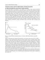
Fig. 6. Cross section of an induction motor (a); Equivalent circuit of an IM (b)
The steady state characteristics of induction machines can be derived from its equivalent
circuit. In order to develop a per phase equivalent circuit of a three-phase machine, a wound
rotor motor as shown in Figure 6.a. is considered here. In case of a squirrel cage motor, the
rotor circuit can be replaced by an equivalent three-phase winding. When three-phase
balanced voltages are applied to the stator, the currents flow in them. The equivalent circuit,
therefore is identical to that of a transformer, and is shown in Figure 6. b. Here R
s
is the
stator winding resistance, L
s
is self inductance of stator, L
r
is self inductance of rotor
winding referred to stator, R
r
is rotor resistance referred to stator, L
m

is magnetizing
inductance and s is the slip. The parameters of the equivalent circuit are the stator and rotor
leakage reactances
s
X

and
r
X

, magnetizing reactance X
m
, and the equivalent resistance
1
Lr
s
RR
s


which depends on the slip s.
The ohmic losses on this “virtual” resistance, R
L,
represent the output mechanical power ,
P
mec
, transferred to the load. Thus the electromagnetic torque , T
e
, is given as
b

i
C

u
C

i
B

u
B

u
u
A

i
a
i
b

i
u
a
u
c

A
a
B

C
c
θ
R
ω
R
α
β
j
X
σs

I
m
U
s

j
X
m
I
r

R
s

jωΨ
s
Jω
s

Ψ
r

I
s

j
X
σ
r

R
r

jω
s
Ψ
m

(a) (b)



sss
LX
;



rsr

LX ;
msm
LX 







rmrsms
LLLLLL ;
s
s
RR
rL


1


Electric Vehicles – Modelling and Simulations

52

22
33
(1 )
(1 )
mec r r

err
ss
pp
PsRR
TII
ss s


 

(9)
If statoric leakage reactance is neglected it results


2
2
2
3
sr
e
s
rslr
URs
Tp
RL










(10)
For applications where high degree of accuracy in speed control is not required simple
methods based on steady state equivalent circuit have been employed. Since the speed of an
induction motor,
n , in revolutions per minute is given by

60
(1 )
s
f
ns
p


(11)
Thus the speed of the motor can be changed by controlling the frequency, or number of
poles or the slip. Since, number of poles of a motor is fixed at the time of construction,
special motors are required with provision of pole changing windings.
4.2.2 The dynamic model of the induction motor
The dynamic model of ac machine can be developed [Ehsani, 2005], [Husain, 2003], using
the concept of “space vectors”. Space vectors of three-phase variables, such as the voltage,
current, or flux, are very convenient for the analysis and control of ac motors and power
converter. A three-phase system defined by
y
A
(t), y

B
(t), and y
C
(t) can be represented uniquely
by a rotating vector
()
y
t in the complex plane.

2
2
3
() ( () () ()) () ()
AB CDQ
y
tytaytaytytjyt
(12)
where

2/3j
ae


Under simplifying assumptions (symmetrical windings with sinusoidal distribution,
negligible cross-section of the conductors, ideal magnetic circuit) the induction squirrel cage
machine may be described in an arbitrary synchronous reference frame, at

g
speed, by the
following complex space vector equations [Livint et all 2006]:


; 0

;
3
;
2
dd
sg rg
uRi j Ri j
sgr gr
sg sg rg
sg rg
dt dt
Li L i L i Li
sm mr
sg rg sg rg
sg rg
d
tpLiiJtDt
em e
sg rg
l
dt


   











    
  

    
(13)
where:
()
;
g
gr
jj
sg s rg r
xxe xxe



;
d
g
g
dt



 - speed of the arbitrary reference frame,
d
r
p
r
dt


 - speed of the rotor reference frame.
In order to achieve the motor model in stator reference frame on impose

g
=0, in equations (13).

Control of Hybrid Electrical Vehicles

53
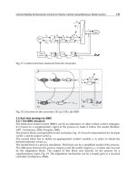
4.3 Power converters
Power converters play a vital role in Hybrid Electric Vehicle (HEV) systems. Typical HEV
drive train consists of a battery, power converter, and a traction motor to drive the vehicle.
The power converter could be just a traditional inverter or a dc-dc converter plus an
inverter. The latter configuration provides more flexibility and improves the system
performance. The dc-dc converter in this system interfaces the battery and the inverter dc
bus, and usually is a variable voltage converter so that the inverter can always operate at its
optimum operating point. In most commercially available systems, traditional boost
converters are used. A power converter architecture is presented in Figure 7.
Voltage source inverters (VSI) are used in hybrid vehicles to control the electric motors and
generators. The switches are usually IGBTs for high-voltage high power hybrid
configurations, or MOSFETs for low-voltage designs. The output of VSI is controlled by

means of a pulse-witth-moduated (PWM) signal to produce sinusoidal waweform. Certain
harmonics exist in such a switching scheme. High switching frequency is used to move the
armonics away from the fundamental frequency.
A three-phase machine being feed from a VSI receives the symmetrical rectangular three-
phase voltages shown in Figure 8.a. Inserting these phase voltage in the space vector
definition of stator voltage


2
2
3
() () () ()
SA SB SC
S
ut u t au t au t, yields the typical set of six
active switching state vectors U
1…
U
6
and two zero vectors U
0
and U
7
as shown in Figure
8.b.

23
2
1, ,6
3

00,7
jk
dc
s
Ue k
u
k










(14)








Fig. 7. Power converter architecture

Electric Vehicles – Modelling and Simulations

54

Fig. 8. a. Switched three-phase waveforms ; b. Switching state vectors
5. Control strategies
A number of control strategies can be used in a drive train for vehicles with different
mission requirements. The control objectives of the hybrid electric vehicles are [Ehsani,
2005]: 1) to meet the power demand of the driver, 2) to operate each component of the
vehicle with optimal efficiency, 3) to recover braking energy as much as possible, 4) to
maintain the state-of-charge (SOC) of the battery in a preset window.
The induction motor drive on EV and HEV is supplied by a DC source (battery, fuel cell, )
which has a constant terminal voltage, and a DC/AC inverter that provide a variable
frequency and variable voltage . The DC/AC inverter is constituted by power electronic
switches and power diodes.
As control strategies PWM control is used for DC motor, FOC (field-oriented control) and
DTC (direct torque control) are used for induction motors. The control algorithms used are
the classical control PID, but and the modern high-performance control techniques: adaptive
control, fuzzy control, neuro network control [Seref 2010], [Ehsani 2005], [Livint et all 2008a,
2008c].
5.1 Structures for speed scalar control of induction motor
5.1.1 Voltage and frequency (Volts/Hz) control
Equation (11) indicates that the speed of an induction motor can be controlled by varying
the supply frequency f
s
. PWM inverters are available that can easily provide variable
frequency supply with good quality output wave shape. The open loop volts/Hz control is
therefore quite popular method of speed control for induction motor drives where high
accuracy in control is not required. The frequency control also requires proportional control
in applied voltage, because then the stator flux

s = U

s
/ω
s
(neglecting the resistance drop)
remains constant. Otherwise, if frequency alone is controlled, then the flux will change.
U
1
=(1,0,0)
U
5
=(0,0,1)
U
6
=(1,0,1)
U
2
=(1,1,0)
U
3
=(0,1,0)
β

U
REF
u
1
u
2
u
D

u
Q
α
ref

U
0
=(0,0,0)
U
7
=(1,1,1)
U
4
=(0,1,1)
(a)
u
sA

u
AZ

u
X
/U
dc

u
BZ

u

CZ

u
OZ

usB

usC

2/3

-2/3

½
-
½
2π
dc link

1 2 3 4
(b)

Control of Hybrid Electrical Vehicles

55
When frequency is increased, the flux will decrease, and the torque developed by the motor
will decrease as shown in Figure 9.a. When frequency is decreased, the flux will increase
and may lead to the saturation of magnetic circuit. Since in PWM inverters the voltage and
frequency can be controlled independently, these drives are fed from a PWM inverter.
The control scheme is simple as shown in Figure 9.b with motor being supplied by three-

phase supply dc-link and PWM inverter.


Fig. 9. a. Torque-speed characeristics under V/f control; b. VSI induction motor drive V/f
controlled
The drive does not require any feedback and is used in low performance applications where
precise speed control is not required. Depending on the desired speed the frequency
command is applied to the inverter, and phase voltage command is directly generated from
the frequency command by a gain factor, and input dc voltage of inverter is controlled.
The speed of the motor is not precisely controlled by this method as the frequency control
only controls the synchronous speed [Emadi, 2005], [Livint et al. 2006] There will be a small
variation in speed of the motor under load conditions. This variation is not much when the
speed is high. When working at low speeds, the frequency is low, and if the voltage is also
reduced then the performance of the motor are deteriorated due to large value of stator
resistance drop. For low speed operation the relationship between voltage and frequency is
given by

0ss
UUkf
(15)
where U
0
is the voltage drop in the stator resistance.
5.2 Structures for speed vector control of induction motor
In order to obtain high performance, and fast dynamic response in induction motors, it is
important to develop appropriate control schemes. In separately excited dc machine, fast
transient response is obtained by maintaining the flux constant, and controlling the torque
by controlling the armature current.
T
e

/ T
base


b
ase
0
1
Constant torque
Constant field
0.5
1.5
1
2
0.5
1.5
2
2.5
Constant power
Weakening region
PWM
∫
+
-
V
*
s
ω
e
*

current
limiting

α
*
i
dc
+
+
ω
sl
ω
*
sleep current
compensation
U
dc
(a)
(b)

Electric Vehicles – Modelling and Simulations

56
The vector control or field oriented control (FOC) of ac machines makes it possible to control
ac motor in a manner similar to the control of a separately excited dc motor. In ac machines
also, the torque is produced by the interaction of current and flux. But in induction motor
the power is fed to the stator only, the current responsible for producing flux, and the
current responsible for producing torque are not easily separable. The basic principle of
vector control is to separate the components of stator current responsible for production of
flux, and the torque. The vector control in ac machines is obtained by controlling the

magnitude, frequency, and phase of stator current, by inverter control. Since, the control of
the motor is obtained by controlling both magnitude and phase angle of the current, this
method of control is given the name vector control.
In order to achieve independent control of flux and torque in induction machines, the stator
(or rotor) flux linkages phasor is maintained constant in its magnitude and its phase is
stationary with respect to current phasor .
The vector control structure can be classified in: 1. direct control structure, when the
oriented flux position is determined with the flux sensors and 2. indirect control structure,
then the oriented flux position is estimated using the measured rotor speed.
For indirect vector control, the induction machine will be represented in the
synchronously rotating reference frame. For indirect vector control the control equations
can be derived with the help of d-q model of the motor in synchronous reference frame as
given in 13.
The block diagram of the rotor flux oriented control a VSI induction machine drive is
presented in Figure 10.
Generally, a closed loop vector control scheme results in a complex control structure as it
consists of the following components: 1. PID controller for motor flux and toque, 2. Current
and/or voltage decoupling network, 3. Complex coordinate transformation, 4. Two axis to
three axis transformation, 5. Voltage or current modulator , 6. Flux and torque estimator, 7.
PID speed controller


Fig. 10. Block diagram of the rotor flux oriented control of a VSI induction machine drive
U
dc
)(ti
sd
)(
*
tu

sC
)(
*
ti
sd
)(
*
ti
sq
)(
*
tu
sA
)(
*
tu
sB
Indirect rotor flux oriented control
)(t
e


)(t
e

)(ti
sq
*
r


Speed sensor
Field weakening
)t(m
*
e
-
)(
*
t
-
-
-

s
L
Speed controller
Current controller

)(t
e


)(
*
tu
sq
)(
*
tu
sd

m
L1
T
K
S
L
PWM
d
q
abc
d
q
abc
i
sA
i
sB
i
sC
)
(
t


)
(
t

Estim
ω

e
, θ
e

Control of Hybrid Electrical Vehicles

57
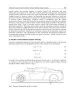
6. Experimental model of hybrid electric vehicle
The structure of the experimental model of the hybrid vehicle is presented in Figure 11. The
model includes the two power propulsion (ICE, and the electric motor/generator M/G)
with allow the energetically optimization by implementing the real time control algorithms.
The model has no wheels and the longitudinal characteristics emulation is realized with a
corresponding load system. The ICE is a diesel F8Q of 1.9l capacity and 64[HP]. The
electronic unit control (ECU) is a Lucas DCN R04080012J-80759M. The coupling with the
motor/generator system is assured by a clutch, a gearbox and a belt transmission.


Fig. 11. The structure of the experimental model of the hybrid electric vehicle
The electric machine is a squirrel cage asynchronous machine (15kW, 380V, 30.5A, 50Hz,
2940 rpm) supplied by a PWM inverter implemented with IGBT modules (SKM200GB122D).
The motor is supplied by 26 batteries (12V/45Ah). The hardware structure of the
motor/generator system is presented in Figure 12. The hardware resources assured by the
control system eZdsp 2808 permit the implementation of the local dynamic control
algorithms and for a CAN communication network, necessary for the distributed control
used on the hybrid electric vehicle, [Livint et all 2008, 2010]
With the peripheral elements (8 ePWM channels, 2x8 AD channels with a resolution of 12
bits, incremental transducer interface eQEP) and the specific peripheral for the

Electric Vehicles – Modelling and Simulations

58
communication assure the necessary resources for the power converters command and for
the signal acquisition in system. For the command and state signal conditioning it was
designed and realized an interface module.
6.1 The emulation of the longitudinal dynamics characteristics of the vehicle
The longitudinal dynamics characteristics of the vehicle are emulated with an electric
machine with torque control, Figure 13. As a mechanical load emulator, the electric machine
operates both in motor and generator regimes. An asynchronous machine with vector
control technique assures a good dynamic for torque. This asynchronous machine with
parameters (15KW, 28.5A, 400V, 1460rpm) is supplied by a SINAMICS S120 converter from
Siemens which contains a rectifier PWM, a voltage dc link and a PWM inverter [Siemens
2007]. This converter assures a sinusoidal current at the network interface and the possibility
to recover into the network the electric energy given by the electric machine when it
operates in generator regime.
The main objective is to emulate the static, dynamics and operating characteristics of the
drive line. The power demand for the vehicle driving at a constant speed and on a flat road
[Ehsani, 2005], can be expressed as

2
,
1
() []
1000 2
evraDfv
te
v
PmgfCAvmgikW


 (16)

Fig. 12. Electric motor/generator system

Control of Hybrid Electrical Vehicles

59

Fig. 13. Emulation system of the longitudinal dynamics characteristics of the vehicle
6.2 The distributed system of the real-time control of the hybrid electric vehicle model
The coordinated control of the sub-systems of the parallel hybrid vehicle can be realized
with a hierarchical structure, [Livint et. al, 2006, 2008]. Its main element is the Electronic
Control Unit vehicle of the vehicle (ECU vehicle) which supervises and coordinates the
whole systems.

It has to monitor permanently the driver demands, the motion conditions and the state of
the sub-systems in order to estimate the optimum topology of the whole system and to
assure minimum fuel consumption at high running performances. The main system must to
assure the maneuverability demanded by the driver in any running conditions. These
supervising and coordinating tasks are realized by a control structure that includes both
state automata elements and dynamic control elements corresponding to each state. The
dynamic control of each sub-system is realized by every local control system. The dynamic
control is integrated at the level of the coordinating system only when it is necessary a
smooth transition between states or for a dynamic change into a state with more than a sub-
system (starting engine with the electric machine).
The optimization of the performances objectives is realized logically by the state automata.
The optimum operating state is determined by the coordinating and supervising system

based on the analysis of the centralized data.
The state machine design is achieved in three stages:
-
the identification of the all possible operating modes of the vehicle,
-
the evaluation of the all possible transitions between the operating modes,
-
the arbitration of the priorities between the concurrent transitions.
For the first stage it is realized a list with the possible operating modes for each sub-system.
For example, for the engine the possible operating modes are running engine and stop engine.

Electric Vehicles – Modelling and Simulations

60
After the identification of the all possible operating modes of each sub-system, it is
generated a set of all the possible combinations of the operating modes for the vehicle.
Due to the complexity of the real time control for a parallel hybrid electric vehicle it is
necessary to integrate all the elements in a high speed CAN communication network
(1Mbps) to assure the distributed control of all resources [CANopen, 2004], [Chacko, 2005].
The experimental model uses a CANopen network with four slave nodes and one master
node. The master node is implemented on phyCORE-mpc555 system and assures the
network management and supervises the nodes control connected by NMT services, the
nodes operating states, the emergency messages analysis and the modifications appeared
into the communication network. The first CANopen slave node, at an inferior level, is
dedicated for the motor/generator system and includes the speed control loop for the
vehicle electrical propulsion.The second slave node is used to take over the torque data
given on the RS-232 serial line by the DTR torque transducer and to convert the data for the
proper utilization on the CANopen network.
The third slave node of the CANopen network is used for the emulation system for the
longitudinal dynamics characteristics of the vehicle, implemented with the asynchronous

motor and the SINAMICS S120 converter.
The fourth slave node of the CANopen network is the system of automatic gear shift,
which involves control of clutch and gear. Control is achieved with a numerical dsPIC-
30F4011.
The CAN protocol utilizes versatile message identifiers that can be mapped to specific
control information categories. With predefined priority of the communication message,
non-destructive bit-wise arbitration with error detection signaling, the CAN protocol
supports distributed real-time control in vehicles applications with a very high level of
security .
The content of a message is named by an identifier. The identifier describes the meaning of the
date, but not indicates the destination of the message. All nodes in the network are able to
decide by message filtering whether the data is to be accepted. If two or more nodes attempt
to transmit at the same time, a non-destructive arbitration technique guarantees the
messages transmission in order of priority and that no messages are lost.
It is guaranteed that a message is simultaneously accepted by all nodes of a CAN network.
When a receiver detects an error in the last bit that cares about it will send an error frame
and the transmitter will retransmit the message.
The CAN network provides standardized communication objects for real-time data (PDO –
Process Data Objects), configuration data (SDO – Service Data objects), and special functions
(Emergency message), network management data (NMT message, Error control).
Service Data Object (SDO) supports the mandatory OD (Object Dictionary) entries, slave
support for the next slave services: Reset_Node, Enter_Preoperational_State,
Start_Remote_Node, Stop_Remote_Node, Reset_Communication, COB (Communication
Data Object).
For the software design it was in attention the modularity and a scalar structure of the
final product that can be easy configured for the automation necessities of the
communication node. For this the CANopen stack was structured in two modules [Livint
et all, 2008, 2009]:
-
Module I, dependent on the hardware resources of the numerical system,

-
Module II, specific for the application, independent on the hardware resources. To pass
the product on other numerical systems it is enough to rewrite the first module.

Control of Hybrid Electrical Vehicles

61
The functional structure of the slave CANopen software is presented in Figure 14.
Module I is specific for the numerical system (phyCORE-mpc555, eZdsp-F2808, dsPIC-
30F4011) and module II is common all three systems.
To implement the CANopen protocol it was used both the graphical programming and the
classic (textual) programming.
6.3 Module I implementation on the eZdsp-F2808 or dsPIC-30F4011 numerical
systems
The Simulink model visible structure of the slave CANopen communication node is
presented in Figure 15.


CANopen Slave
PDO
Management
APPLICATION
User interface
- Configurations
- Function calls
Transceive
r
CAN Controller
SDO Server NMT Slave

PDO Mapping
Signaling
- Diagnosis
- Operating state
CAN Controller
Mana
g
emen
t

MODULE I
MODULE II
CONFIGURATION MODULE
CAN network

Fig. 14. The functional structure of a CANopen slave
The CANOpen Message Receive (dsPIC30F4011 or eZdsp 2808) sub-system realizes the
messages reception into the CANopen stack buffer. The messages are transmitted by the
CANOpen Message Send (dsPIC30F4011 or eZdsp 2808) sub-system.
They are part of the Module I from the Figure 16. In the same module there is also the
CANOpen Err & Run LED’s sub-system which commands the two LEDs of the numerical
system. The stack initialization and its periodical interrogation are realized by the Init
CANOpen, and SW_TimerISR sub-systems.
The data transfer between the graphical and textual modules is made with global variables
which are defined by the state flow chart. It is to mention that was necessary to interfere
with the C-code generating files (Target Language Compiler – TLC) to obtain the necessary
functionability.
An important aspect of the CANopen implementation is the generation of relative
references of time to administrate the data transfer messages (timestamp) and the
administrative data (node guarding, heartbeat).For this it was used a software which call

both the CANopen stack and the timer with 1 ms period.

Electric Vehicles – Modelling and Simulations

62
Module I implementation on phyCORE-mpc555 numerical system
The Simulink model for the CANopen node of the second numerical system is similar with
the model from Figure 17 but eZdsp 2808 is changed with phyCORE-mpc 555. Thus, for a
user which knows a model it is easy to operate with the other. The communication speed is
established with the MPC555 Resource Configuration module.
Module II implementation of slave CANopen communication node
The graphical programming is operative and suggestive. It also has limits especially for the
complex algorithms processing. In this case the programmer makes a compromise:
hardware resources are realized with the graphical libraries and the complex algorithms
processing are implemented with textual code lines. The Matlab/Simulink embraces such a
combined programming.
Thus, the second module was implemented by a textual programming. The function call is
realized with a 1KHz frequency by the SW_TimerISR sub-system. SDO services are
assured by the object dictionary SDOResponseTable and by the functions Search_OD
(WORD index, BYTE subindex), Send_SDO_Abort (DWORD ErrorCode) and
Handle_SDO_Request (BYTE*pData). The functions Prepare_TPDOs (void) and
TransmitPDO (BYTE PDONr) realize the administration of the data transmission
messages between the numerical systems
The node initialization is realized by the function CANOpen_Init (BYTE Node_ID, WORD
Heartbeat) and the communication network administration (NMT slave) are incorporate
into the function CANOpen_ProcessStack(void).
The connections (mapping) between the data on the CAN communication bus can be static
realized by the initialization function CANOpen_InitRPDO (BYTE PDO_NR, WORD
CAN_ID, BYTE len, BYTE *dat), CANOpen_InitTPDO (BYTE PDO_NR, WORD CAN_ID,
WORD event_time, WORD inhibit_time, BYTE len, BYTE *pDat).

Fig. 15. The Simulink model assigned to the slave CANopen communication node

Control of Hybrid Electrical Vehicles

63
6.4 Experimental results
In Figure 16 is presented the hybrid electric vehicle model realized into the Energy
Conversion and Motion Control laboratory of the Electrical Engineering Faculty from Iasi.
Finally several diagrams are presented highlighting the behaviour of the electric traction
motor and the mechanical load emulator. It was considered a standard operating cycle
UDDS (Urban Dynamometer Driving Schedule).
A velocity diagram UDDS cycle operation is shown in Figure 17-a. It is the speed reference
for electric traction motor and the measured speed is presented in Figure 17-b.



Fig. 16. Hybrid electric vehicle experimental model



Fig. 17. a) Reference speed for UDSS cycle b) Measured speed for electrical motor
eZds
p

dsPIC30F4011
m
p

c555
ECU ICE
Sinamics

Electric Vehicles – Modelling and Simulations

64
The active current from electrical traction motor is shown in Figure 18-a. Also the
mechanical load emulator is an electrical motor with torque control and the torque reference
shown in Figure 18-b. In Figure 19 is presented the estimated torque from mechanical load
emulator.


Fig. 18. a) The active current from electric traction motor b) The reference torque for
Sinamics system


Fig. 19. The estimated torque from mechanical load emulator
7. Conclusions
The hybrid electric vehicles are very complex dynamic systems and have an important
number of interconnected electrical systems to achieve the required operating performances.
Because of the complexity of the real time control for a hybrid electric vehicle it is necessary
to integrate all the elements in a high speed CAN communication network to assure the
distributed control of all the resources. For the hybrid electric vehicle experimental model is
used a CANopen network with one master node and four slave nodes. The distributed
system control with the CANopen protocol on a CAN bus permits the control of the
electrical drives systems in safe conditions and with improved dynamic performances.

Control of Hybrid Electrical Vehicles

65
8. References
Bayindir , K. C., Gozukucuk, M.A., Teke, A. , (2011). Acomprehensive overwiew of hybrid
electric vehicle: Powertrain configurations, powertrain control techniques and
electronic control units, Energy Conversion and Management, Elsevier, nr. 52, 1305-
1313.
CANopen, User Manual, Software Manual, (2004), PHYTE Technology Holding Company
Chacko, V.R., Lahaparampil, V.Z., Chandrasekar, V., (2005). CAN based distributed real
time controller implementation for hybrid electric vehicle, IEEE, 247- 251, ISBN 0-
7803-9280-9-05
Chan, C.C, (2002), The state of the art of electric and hybrid vehicles, Proc. IEEE, vol. 90, no.
2, pp. 247–275
Comigan , S., (2002). Introduction to the Controller Area Network (CAN), Texas Instruments
Application Report, SLOA101-August 2002, pp. 1-16
Duan, J., Xiao, J., Zhang, M., (2007). Framework of CANopen protocol for a hybrid electric
vehicle, Proceedings of the IEEE Intelligent Vehicles Symposium, Instanbul, Turkey,
June 13-15, 2007.
Ehsani M., Gao Y., Gay E.S. Emadi A, (2005). Modern Electric, Hybrid Electric, and Fuel Cell
Vehicles CRC PRESS, Boca Raton London, New York, ISBN 0-8493-3154-4
Emadi Ali, (2005). Hanbook of Automotive power electronics and MotorDrives, CRC PRESS,
Taylor&Francis Group, LLC, 2005, ISBN 0-8247-2361-9
Fuhs A.E., (2009). Hybrid Vehicles, CRC PRESS 2009, Taylor Francis Group, LLC,ISBN 978-1-
4200-7534-2
Guzzella L., Sciarretta A., (2007). Vehicle Propulsion Systems, Second Edition, Springer-Verlag
Berlin Heidelberg, ISBN 978-3-540-74691-1
Husain I., (2003), Electric and Hybrid Vehicles Design Fundamentals, CRC PRESS, ISBN 0-8493-
1466-6
Livint, Gh., Gaiginschi, R., Horga, V., Drosescu R., Chiriac, G., Albu, M., Ratoi, M., Damian,
I, Petrescu M., (2006). Vehicule electrice hibride, Casa de Editura Venus, Iasi, Romania
Livinţ, Gh., Răţoi, M., Horga, V., Albu, M, (2007). Estimation of Battery Parameters Based on

Continuous-Time Model, Proceedings International Symposium on Signals,
Circuits&Systems-ISSCS , July 12-13, 2007, Iasi, Romania, pp. 613-617, IE.EE. Catalog
Number: 07EX1678C, ISBN: 1-4244-0969-1
Livinţ Gh., Horga, V., Albu, M., Răţoi, M, (2007). Evaluation of Control Algorithms for
Hybrid Electric Vehicles, WSEAS TRANSACTIONS on SYSTEMS, Issue 1, Vol. 6,
January 2007, pp. 133-140, ISSN 1109-2777,
Livint, Gh., Horga, V., Ratoi, M., (2008), Distributed control system for a hybrid electric
vehicle implemented with CANopen protocol, -Part I, Bulletin of the Polytechnic
Institute of Iasi, Tom LIV (LVIII), FASC. 4, ISSN 1223-8139, pp. 1019-1026
Livint, Gh., Horga, V., Ratoi, M., Albu, M., Petrescu, M., Chiriac, G., (2008). Distributed
control system for a hybrid electric vehicle implemented with CANopen protocol-
Part II, Bulletin of the Polytechnic Institute of Iasi, Tom LIV (LVIII), FASC. 4, ISSN
1223-8139, pp. 1027-1032
Livint, Gh., Horga, V., Ratoi, M., Damian, I., Albu, M., Chiriac, G., (2008). Advanced real
rime control algorithms for hybrid electric vehicles optimization, CEEX Program,
Simposion “Contributii Stiintifice ”, UCP AMTRANS, Bucuresti, Romania, noiembrie
2008, pp. 209-214

Electric Vehicles – Modelling and Simulations

66
Livint, Gh., Horga, V., Ratoi, M., Albu, M., Chiriac, G., (2009), Implementing the CANopen
protocol for distributed control for a hybrid electric vehicle, Proceedings The 8th
International Symposium on Advanced Electromechanical Motion Systems, Lille , July 1-
3, CD., ISBN: 978-2-915913-25-5/EAN: 978-2-91 5913-26-5 IEEExplore,

Livinţ, Gh., Horga, V., Sticea, D., Raţoi, M., Albu, M., (2009) Electrical drives control of a
hybrid electric vehicle experimental model, Proceedings of the 7
th
International

Conference of Electromechanical and Power Systems, Editura PIM, 2009, vol. II, pp. 21-
27, ISBN vol II, 978-606-520-623-6, October 8-9, 2009, Iaşi, Romania,
Livinţ Gh., Horga V., Sticea D.,Raţoi M., Albu M., (2010). Hybrid electric vehicle
experimental model with CAN network real time control, in Advances in Eectrical
and Computer Engineering, nr. 2., 2010, pp. 102-108, ISSN 1582-7445, Stefan cel Mare
University of Suceava, Romania
Petrescu, M., Livinţ, Gh., Lucache, D. (2008), Vehicles dynamic control using fuzzy logic,
Proocedings of 9th WSEAS International Conference on Automation and Information,
pag. 488-493, 2008
Seref Soylu, (2010) Urban Transport and Hybrid Vehicles, Published by Sciyo, Janeza Trdine 9,
51000 Rijeka, Croatia, ISBN 978-953-307-100-8
Siemens, Sinamics, S120 Control Unit and additional system components, (2007), Equipment
Manual 03, Edition
Sticea D., Livinţ Gh., Albu M., Chiriac G., (2009). Experimental stand for the dynamical cycle
study of the batteries used on hybrid electrical vehicle, Proceedings of the 7
th

International Conference of Electromechanical and Power Systems, Editura PIM, 2009,
vol. II, pp. 172-175, ISBN vol II, 978-606-520-623-6, October 8-9, 2009, Iaşi, Romania,
Yamada, E., and Zhao, Z., (2000). Applications of electrical machine for vehicle driving
system, Proceedings of the Power Electronics and Motion Control Conference (PIEMC),
vol 3., pp. 1359-1364, Aug. 15-18, 2000.
Westbrook H. M., (2005). The Electric Car, Developmrent and future of battery, hybrid and fuel-
cell cars, The Institution of Electricl Engineers, London, 2005, ISBN 0 85296 013 1
Wyczalek, F.A., (2000) Hybrid electric vehicles year 2000, Proceedings of the Energy
Conversion Engineering Conference and Exhibit (IECEC) 35
th
Intersociety, vol.1,
pp. 349-355, July 24-28, 2000
4

Vehicle Dynamic Control of 4 In-Wheel-Motor
Drived Electric Vehicle
Lu Xiong and Zhuoping Yu
Tongji University
China
1. Introduction
Thanks to the development of electric motors and batteries, the performance of EV is greatly
improved in the past few years. The most distinct advantage of an EV is the quick and
precise torque response of the electric motors. A further merit of a 4 in-wheel-motor drived
electric vehicle (4WD EV) is that, the driving/braking torque of each wheel is independently
adjustable due to small but powerful motors, which can be housed in vehicle wheel
assemblies. Besides, important information including wheel angular velocity and torque can
be achieved much easier by measuring the electric current passing through the motor. Based
on these remarkable advantages, a couple of advanced motion controllers are developed, in
order to improve the handling and stability of a 4WD EV.
2. Traction control
The fast and accurate torque generation of each driving wheel enables a great enhancement
in traction control during acceleration.
In this section, an anti-slip controller for a 4WD EV using VSC (Variable Structure Control)
method is presented. The control algorithm is independent on the identification of the road
adhesion coefficient and has excellent robustness to the estimation error of the vehicle velocity.
Regarding the high-frequency-chattering on the sliding surface, a new control method which
combines the advantage of the VSC and MFC (Model Following Control) in order to decrease
the fluctuation to the e-motor torque and slip ratio of the tire is proposed. The result of the
simulation indicates that the proposed control method is effective for the ASR control and
improves the performance of e-motor’s output torque and the slip ratio of the tire.
2.1 VSC ASR controller
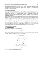
2.1.1 One-wheel-model
An accurate simulation model is important to verify the effect of the designed controller.
Fig.2.1-1 shows a two degrees of freedom vehicle model. It only contains the vehicle’s

longitudinal motion and ignores air resistance and rotating resistance. Formula 2.1-1 shows
the mathematical model:
x
d
M
vF




Electric Vehicles  Modelling and Simulations

68

wmx
ITFR


 (2.1-1)
Here, M is the 1/4 vehicle mass, kg; v
x
represents the longitudinal velocity, m/s; F
x
is the
driving force of the road, N; I
ω
is the wheel rotational inertia, kg·m
2
; R is the wheel radius,
m; ω is the angular velocity, rad/s and T

m
is the motor torque, N·m.
The Magic Formula tire model is applied as the tire model, so the driving force F
d
can be
expressed as follows:






sin arctan 1 arctan( )
dMaxZ
FFCBEEB


   (2.1-2)
The meanings of the parameters can be found in the literature
[1]
.


Fig. 2.1-1. One-wheel-Model
2.1.2 Design of VSC ASR controller
VSC with sliding mode has good robustness to the input signals so that this strategy has
advantage to the ASR control system which needs the vehicle velocity observation and
signal identification. But there is always high-frequency-chattering on the sliding surface. In
the following text a VSC controller, which doesn’t depend on the identification of the
optimal slip ratio, is designed and its performance will be analyzed through simulation.

In order to make the VSC possess excellent robustness to the additional uncertainties and
interferences, the control law adopted here is equivalent control with switching control.
Hence, the output torque of the e-motors can be expressed as
[2]
:

,
s
g
n( )
mmeq
TT T s

 (2.1-3)
In this equation, T
m,eq
is the equivalent torque of the e-motor, ΔT is the hitting control drive
torque, sgn(s) is the switching function of the system.
The sliding motion includes two processes: approaching motion and sliding motion. The
approaching motion can make the system at any time in any position approach to the
sliding face in limited time. The sliding motion occurs only when the system reaches sliding
surface:
0
reference
s



.

Vehicle Dynamic Control of 4 In-Wheel-Motor Drived Electric Vehicle

69

Fig. 2.1-2. Diagram of VSC ASR Strategy
To reach the ideal sliding mode, the requirement s=0 should be fulfilled. Assuming the
reference slip is constant, so
.
0
reference



So, on the sliding face there is:
0
reference



 (2.1-4)
According to the one-wheel model:
mx
ITFR




During driving process, the slip ratio of the wheel can be expressed as:
Rv
R







Combining Formula (2.1-1) and (2.1-4), we can get:
1
(1 ) 0
mx
TFR
d
vR
dt R I








 



Then, we can obtain the e-motor’s equivalent torque:
,
(1 )
me

q
x
I
TvFR
R






As the tire’s longitudinal velocity is difficult to be measured accurately,
v

is the estimated
value. Then the above formula can be rewritten as:

,
(1 )
meq
x
I
TvFR
R







(2.1-5)
In the actual driving progress, there are many kinds of road surfaces and their respective
optimal slip ratios. The identification for them is difficult. Through Fig. 2.1-3, we can see that,
although the slip ratios for different roads are different, the basic shapes for μ-λ curves are

Electric Vehicles  Modelling and Simulations

70
similar. It means, before the optimal slip ratio, the bigger the slip ratio, the larger the
longitudinal adhesion coefficient is. While after the optimal slip ratio, the bigger the slip
ratio, the smaller the longitudinal adhesion coefficient is
[3]
.


Fig. 2.1-3. Slip ratio-Longitudinal adhesion coefficient on different road surface
From Fig. 2.1-3, we can get:
When
d
0
d



,
re
f
erence




,

needs increasing so as to get larger adhesion coefficient and
the driving torque should be increased.
When
d
0
d



,
re
f
erence


 ,

needs keeping so as to get larger adhesion coefficient and the
driving torque should be maintained.
When
d
0
d



,

re
f
erence



,

needs decreasing so as to get larger adhesion coefficient and
the driving torque should be reduced.
According to the one-wheel model, we can acquire:
m
Z
TI
FR







Then we can get:
2
2
/
.
/
()
m

m
Z
Z
TI
TI
dddt
FR
dddt F
vR v R v v
R




 











 


Now, we can get the judgment condition:

When
0
m
TI
vv








, the e-motor’s output torque needs increasing;

Vehicle Dynamic Control of 4 In-Wheel-Motor Drived Electric Vehicle

71
When 0
m
TI
vv









, the e-motor’s output torque needs keeping;
When
0
m
TI
vv








, the e-motor’s output torque needs decreasing.
From above we can find that what the switching function needs is not the slip ratio and the
reference slip ratio any more, but the angular speed, e-motor’s torque and driving torque,
which need not identification. Although there is still longitudinal velocity estimation value
in the controller, the controller itself has solved this problem which can be seen in Formula 8.
So this VSC strategy is considered as feasible.
When the system is not on the sliding surface, it needs approaching the sliding surface from
any state. This motion is called approaching motion. And during this motion the slip ratio
will be approaching 0.
Under the generalized sliding condition, the switching function should meet:

ss s


 (2.1-6)
Here the parameter


>0.

represents the velocity, in which the system approaches the
sliding surface. The larger the

is, the faster the approaching velocity is. Whereas, the
chattering on the sliding surface will be bigger.
When Formula (2.1-1) is put into Formula (2.1-6), we can get:

sgn( )
[(1 ) ]
mx
TT sFR
s
vR s
RI






 
 
(2.1-7)
Here the hitting control driving torque is assumed as

()
(1 )

I
TF







(2.1-8)
Putting Formula 2.1-7 into Formula 2.1-6, we can get:

1
()
xx
vvsFs
R





That is:

1
xx
Fvv
R





 (2.1-9)
So the e-motor’s output torque can be shown as

,
s
g
n( )
m
meq
TT T s

 (2.1-10)

Electric Vehicles  Modelling and Simulations

72
The simulation results for vehicle that starts on the road surface with a low adhesion
coefficient
（μ=0.2）is shown in Fig.2.1-4.




Fig. 2.1-4. Start on a low adhesion surface
（μ=0.2）
From the simulation results we can get that the vehicle can keep away from skipping and
the acceleration performance is good when it starts. But the slip ratio occurs fluctuation
when it’s among 0 to 0.3 and the e-motor’s output torque also fluctuates near 300Nm. In

reality, big fluctuation is harmful to the e-motor and sometimes the e-motor can’t fully
realize what the controller requires. Therefore, there are some defects in this method.

Vehicle Dynamic Control of 4 In-Wheel-Motor Drived Electric Vehicle

73
2.2 ASR combined controller
2.2.1 MFC controller
According to the research results from Tokyo University
[4, 5]
, when the tire is completely
adhered, the vehicle’s equivalent mass is equal to the sum of the sprung mass and non-
sprung mass. When the tire slips, the angular speed changes significantly. During
acceleration, the angular speed is obviously smaller than the ideal value which is outputed
by the standard model. In light of this principal, the tire’s angular speed should be
compared to the angular speed from the standard model at any time. And then the
difference is used as the basis for a correction value through a simple proportional control to
adjust the e-motor’s output torque. So that the tire can avoid slipping.
MFC strategy only requires the e-motor’s output driving torque and the tire’s angular speed
signal to put ASR into practice. Consequently the estimation of the longitudinal velocity and
the optimal slip ratio identification can be ignored. Therefore, this strategy is practical. The
system diagram is shown in Fig.2.2-1.

1
w
ms
1
1s



d
F
-
+
M
F
M
F

w
V
-
+
+
-
dF


w
mms
1
()
w
mms


Fig. 2.2-1. MFC control block diagram
The standard model of MFC is got under the condition that the slip ratio is set to 0. It means
that the road’s adhesion force isn’t fully utilized and the driving performance will be bad. So
this control strategy is not perfect. Secondly, MFC hasn’t good robustness to the input

signals. Especially when the angular speed is disturbed, deviation of the controller will
happen.
2.2.2 Combined controller
Based on the characters of VSC and MFC, in this section an area near the sliding surface will
be set, within which the MFC strategy is applied. And out of this area, the VSC strategy is
used.Thus, the high-frequency-chattering near the sliding surface can be avoided. The
system diagram is shown in Fig.2.2-2 and Fig.2.2-3.