Evaporation Condensation and Heat transfer Part 11 docx
Bạn đang xem bản rút gọn của tài liệu. Xem và tải ngay bản đầy đủ của tài liệu tại đây (823.29 KB, 40 trang )
16 Heat Transfer
HTR% HTR%/DR%
Pr 0.1 1.0 2.0 0.1 1.0 2.0
Case 2 8.0% 16.6% 16.3% 0.39 0.80 0.79
Case 3a 49.9% 58.5% 62.3% 0.79 0.93 0.99
Case 3b 47.2% 57.3% 64.9% 0.68 0.82 0.93
Case 4 54.0% 69.3% 72.8% 0.75 0.97 1.02
Table 3. Heat-transfer reduction rates and ratio relative to drag-reduction rate
reason, the m agnitude of HTR% obtained at Pr
= 0.1 was relatively low compared with DR%,
as shown below.
Figure 8 further indicates that θ
+
rms
in case 2 is slightly increased from that in case 1 (5 < y
+
<
70). It can be considered that the influence of the turbulence modulation due to the fluid
viscoelasticity occurs there and does not exist in the core region (70
< y
+
).
3.4 Reduction rate of heat transfer
Table 3 shows the percentage of heat-transfer reduction, HTR%, and the ratio of HTR to DR.
The rate of HTR% is calculated with the following equation:
HTR%
=
Nu
K
− Nu
Nu
K
× 100% (27)
where Nu
K
is the Nusselt number at the same bulk Reynolds number predicted by an
empirical correlation function for Newtonian fluid:
Nu
K
= 0.020Pr
0.5
Re
0.8
m
. (28)
This equation has often been used for evaluating heat-transfer correlations in channel flow.
Note that we applied t he coefficient 0.020, which was recommended by Tsukahara et al.
(2006), in place of 0.022 originally given by Kays & Crawford (1980); however, we used 0.025
for Pr
= 0.1 to ensure a consistency with the Newtonian case.
For a unit value of Prandtl number (Pr
= 1.0), the obtained HTR%isatthesameorderof
magnitude as DR% in each case (see Table 3). As described previously, there are two types
of factor causing DR. One is the suppression of turbulence under high We
τ
(e.g. case 4 in
particular), and the other is the diminution in effective viscosity under low β (case 3b). We can
expect that the HTR in case 4 should also be enhanced, giving rise to a high HTR%, because
the turbulent motion promotes heat transfer as well as momentum transfer. In contrast, in
case 3b, no significant change in HTR% was observed compared with that in case 3a, whereas
the difference of DR% between the cases was relatively large. Both DR%andHTR%were
increased as We
τ
was increased at a constant β, while only DR%, rather than both, was
increased with decreasing β. From the comparison with other Prandtl numbers, a similar
tendency can be observed: the highest-HTR% flow was in case 4, and case 3b showed almost
identical HTR% with that in case 3a.
As can be seen from Table 3, the obtained values of HTR%forPr
= 0.1 are much smaller than
DR%andHTR% for moderate Prandtl numbers. This is due to the low Prandtl-number effect,
as discussed in section 3.6, where we examine the statistics related to turbulent heat flux. The
HTR-to-DR ratio is also shown in Table 3, showing values smaller than 1 except for case 4 at a
relatively high Prandtl number. According t o the results, the fluid condition in case 3b can be
390
Evaporation, Condensation and Heat Transfer
Turbulent Heat Transfer in Drag-Reducing
Channel Flow of Viscoelastic Fluid 17
10
-2
10
-1
10
0
10
0
10
1
10
2
Pr
Nu
Present
Case 1
Case 2
Case 3a
Case 3b
Case 4
Nu ~ Pr
0.4
DNS at Re
τ
=180
Kawamura et al. (1998)
Kozuka et al. (2009)
Sleicher & Rouse (1975)
Re
τ
=150
10
3
10
4
Re
m
Laminar value
Kozuka et al. (2009)
DNS at Pr = 2.0
Present
Pr=2.0
Pr=1.0
Pr=0.1
Pr
2.0
1.0
0.1
Nu ~ Pr
0.4
Re
m
-1
Fig. 9. Relationship between Nusselt and Prandtl numbers. DNS results by other researchers
and a turbulent relationship for Newtonian flow are shown for comparison.Relation between
Nusselt and Reynolds numbers. The laminar value of 4.12 and a turbulent relationship for
Newtonian flow are shown for comparison.
adequate to avoid attenuation of turbulent heat transfer. However, the low Prandtl-number
condition might not be practically interesting, since water (with Pr
= 5–10) is often used
as the solvent of drag-reducing flows. Aguilar et al. (1999) experimentally observed that,
in drag-reducing pipe flow, the HTR-to-DR ratio decreased at higher Reynolds number and
stabilized at a value of 1.14 for Re
m
> 10
4
. Our results showed much lower values than their
measurements, but exhibited certain Prandtl-number dependence, that is, the HTR-to-DR
ratio was a function of the Prandtl number.
Figure 9 shows the Prandtl-number and Reynolds-number dependences of the Nusselt
number. It is practically important to compare the results for the heat transfer coefficient in
drag-reducing flow with those predicted by widely used empirical correlations for Newtonian
turbulent flows. The empirical correlation in terms of the Pr dependence suggested by
Sleicher et al. (1975) is shown as a dotted line in the left figure. Note that this correlation
is originally for the pipe flow; moreover, the present Reynolds number is smaller than its
applicable range. The present results are lower than the correlation because of the low
Reynolds-number effect. We also present a fitting curve of Pr
0.4
shown by the solid line in
the same figure. The results for case 1 collapse to this relationship as well as other DNS data
(Kawamura et al., 1998; Kozuka et al., 2009), although a slight absolute discrepancy arises
because of the difference in Re
τ
. As for the viscoelastic flows, the obtained Nu are smaller
than the correlation, especially at moderate Prandtl numbers. It is interesting to note that the
correlation of Nu ∝ Pr
0.4
is still applicable in the range of Pr = 1–2, even for the drag-reducing
flows.
We plot in the right figure (Nu versus Re
m
) the corresponding values of Nu
K
for Newtonian
turbulent flow predicted by Equation (28). The relationship in case 1 (at Re
m
= 4650)
shows good agreement with the empirical correlation. It is found that in viscoelastic flow
391
Turbulent Heat Transfer in Drag-Reducing Channel Flow of Viscoelastic Fluid
18 Heat Transfer
Nu decreases as Re
m
increases, revealing a trend quantitatively opposite to that estimated by
the correlation as the following form:
Nu ∝ Pr
0.4
Re
−1
m
. (29)
It is clearly confirmed from Fig. 9 that Equation (29) shows much better correlation of the data
at Pr
= 1–2 for cases 2, 3a, and 4 (i.e., varying We
τ
with a constant β). The obtained Nu in case 2
(at Re
m
= 8860) is significantly larger than that in the Equation (29). This also suggests that the
decrease of β gives rise to DR% with relatively small HTR% compared to a case of increasing
We
τ
.ThevaluesatPr = 0.1 are much larger than those with Equation (29), approaching
the laminar value of Nu
= 4.12. Hence the turbulent heat transfer of drag-reducing flow at
low Prandtl numbers may be qualitatively different from t hat for moderate Prandtl numbers.
From a practical viewpoint, these findings are also useful. As the Nu appeared to be a unique
function of Re
m
and Pr even for a wide range of fluids (i.e., different relaxation times of
viscoelastic fluid), one can readily predict the level of HTR on the basis of measurements
of DR%.
3.5 Reduced contribution of turbulence to heat transfer
As shown in Tables 1 and 3, non-negligible DR%andHTR% are obtained in case 2, although
the attenuation of the momentum and heat transport seems to be small and limited in the
near-wall region (see also Fig. 8). In addition, a large amount of HTR is achieved in the
highly drag-reducing flow (cases 3–4), where near-wall turbulent motion is suppressed and
the elastic layer develops. These features occur because the wall-normal turbulent heat flux
as well as the Reynolds shear stress in the near-wall region should primarily contribute to
the heat transfer and the frictional drag, in the context of the FIK identity (see Fukagata et al.,
2002; 2005; Kagawa, 2008).
From Equation (16), the total and wall-normal turbulent heat flux can be obtained by ensemble
averaging as follows:
q
total
= 1 −
y
0
u
u
m
dy
=
1
Re
τ
Pr
∂
θ
+
∂y
− v
+
θ
+
. (30)
By applying integration of
1
0
(1 − y
)d y
, the above equation can be rearranged as follows:
1
2
− A =
Θ
+
Re
τ
Pr
+
1
0
(1 − y
)
−v
+
θ
+
dy
, (31)
where
A
=
1
0
(1 − y
)
y
0
u
u
m
dy
dy
, Θ
+
=
1
0
θ
+
dy
. (32)
Then, the relationship between the inverse of the Nusselt number (namely, the dimensionless
thermal resistance of the flow) and the turbulence contribution (wall-normal turbulence heat
flux) is given as follows:
R
≡
1
Nu
=
θ
+
m
2Re
τ
Pr
= R
mean
− R
turb
(33)
R
mean
=
θ
m
2Θ
1
2
− A
(34)
R
turb
=
θ
m
2Θ
1
0
(1 − y
)
−v
+
θ
+
dy
. (35)
392
Evaporation, Condensation and Heat Transfer
Turbulent Heat Transfer in Drag-Reducing
Channel Flow of Viscoelastic Fluid 19
40%
50%
60%
70%
80%
90%
100%
R
R
turb
b
ution of thermal resistance
0%
10%
20%
30%
40%
50%
60%
70%
80%
90%
100%
Case 1 Case 2 Case 3a Case 3b Case 4
R
R
turb
Fractional contribution of thermal resistance
Fig. 10. Fractional contribution of thermal resistance (inverse of Nusselt number) for Pr = 1.0.
Here, R
mean
corresponds to the resistance estimated from mean velocity and temperature.
This identity function indicates that R can be interpreted as the actual thermal resistance,
which is obtained by subtraction of the negative resistance (R
turb
) due to turbulence from
R
mean
. For larger turbulent heat flux near the wall, the term R
turb
increasesandplaysan
important role to decrease the thermal resistance.
In order to examine the thermal resistance under the present conditions, the components
of thermal resistance in Equation (33) are shown in Fig. 10. Note that R
mean
,thatis,
the sum of the actual thermal resistance R and the turbulence contribution R
turb
, is 100%.
Only a single Prandtl number of 1.0 is presented, but similar conclusions can be drawn for
Pr
= 2.0. Generally, R
turb
is as much as half of R
mean
and suppresses the actual thermal
resistance. An increase of R should give rise to an increase of HTR%. As expected, the
viscoelastic flows reveal smaller fractions of R
turb
relative to the Newtonian flow of case 1,
It is interesting to note that no difference is found in the results between cases 3a and 3b,
where the same Weissenberg number is given. This is consistent with HTR%, which is almost
identical for both cases. I n Fig. 10, R
turb
is apparently decreased as We
τ
changes from 0 to
10
→ 30 → 40. It can be concluded that the actual thermal resistance significantly depends on
the Weissenberg number. In the following section, the cross correlation with respect to velocity
and temperature fluctuations is discussed to investigate the diminution of the wall-normal
turbulent heat flux contained in the component shown in Equation (35).
3.6 Cross-correlation coefficients.
Figure 11 shows the cross-correlation coefficient between the fluctuating velocity in the
streamwise direction and the fluctuating temperature. This coefficient is defined as follows:
R
uθ
=
u
θ
u
rms
θ
rms
. (36)
The profile of R
uθ
as a function of y
+
is reported in Fig. 11. The R
uθ
for the viscoelastic
flows is fairly constant f rom 0.8 to 0.96 in most of the channel, while that in case 1
decreases monotonically there. This result means that, even in the outer region, the
393
Turbulent Heat Transfer in Drag-Reducing Channel Flow of Viscoelastic Fluid
20 Heat Transfer
0 50 100 150
0.5
0.6
0.7
0.8
0.9
1
Case 1
Case 2
Case 3a
Case 4
y
+
R
u
θ
10
0
10
1
0.85
0.9
0.95
1
Case 1
Case 3a
Case 3b
0 50 100 150
0.5
0.6
0.7
0.8
0.9
1
Case 3a
Case 3b
y
+
R
u
θ
Fig. 11. Cross-correlation coefficient between fluctuations of u
and θ
for Pr = 1.0.
0 50 100 150
0
0.1
0.2
0.3
0.4
0.5
0.6
–R
uv
–R
v
θ
Case 1
Case 2
Case 3a
Case 4
y
+
–R
uv
, –R
v
θ
0 50 100 150
0
0.1
0.2
0.3
0.4
0.5
0.6
–R
uv
–R
v
θ
Case 3a
Case 3b
y
+
–R
uv
, –R
v
θ
10
0
10
1
0.1
0.2
0.3
0.4
Fig. 12. Same as Fig. 11 but for v
and u
,orv
and θ
.
temperature fluctuations are better correlated with the streamwise velocity fluctuations than
the Newtonian case. Also note that the good match between cases 3a and 3b appears in
the entire channel except in the vicinity of the wall, namely, in the viscous sublayer. This
is consistent with above discussions in the sense that the cases are different in terms of
the viscous-sublayer thickness and that the mean temperature profiles are comparable when
scaled with y
+
,noty
∗
.
As mentioned above, the wall-normal turbulent heat flux is reduced for
high-Weissenberg-number flows, despite the increased temperature var iance (shown i n
Fig. 8). It can thus be conjectured that the turbulent heat flux of
−v
θ
should be influenced
by the loss of correlation between the two variables. Fig. 12 shows the cross-correlation
coefficients of the wall-normal turbulent heat flux and of the Reynolds shear stress:
R
vθ
=
v
θ
v
rms
θ
rms
, R
uv
=
u
v
u
rms
v
rms
. (37)
For cases 3–4, both R
vθ
and R
uv
are much smaller t han those in case 1, throughout the channel.
The peak values are almost 20%–30% lower than the ones obtained in case 1. The profiles of
394
Evaporation, Condensation and Heat Transfer
Turbulent Heat Transfer in Drag-Reducing
Channel Flow of Viscoelastic Fluid 21
R
vθ
and R
uv
for each case exhibit similar shapes throughout the channel, which also implies
similarity between the variations of
−v
θ
and −u
v
affected by DR. These features at Pr = 1.0
can be seen also at the other Prandtl numbers (figure not shown) and also agree well with
those of experimental results and DNS for water (Gupta et al., 2005; Li et al., 2004a). This less
correlation between θ
and v
is responsible for the decrease of the wall-normal turbulent heat
flux and the increase of HTR%, in the same way that the decrease of the Reynolds shear stress
due to the lower correlation between u
and v
should be responsible for DR%.
4. Conclusion
A series of direct numerical simulations (DNSs) of turbulent heat transfer in a channel flow
under the uniform heat-flux condition have been performed at low friction Reynolds number
(Re
τ
= 150) and various Prandtl numbers in the range of Pr = 0.1 to 2.0. In order to
simulate viscoelastic fluids exhibiting drag reduction, the Giesekus constitutive equation
was employed, and we considered two rheological parameters of the Weissenberg number
(We
τ
), which characterizes the relaxation time of the fluid, and the viscosity ratio (β)ofthe
solvent viscosity to the total zero-shear rate solution viscosity. Several statistical turbulence
quantities including the mean and fluctuating temperatures, the Nusselt number (Nu), and
the cross-correlation coefficients were obtained and analyzed with respect to their dependence
on the parameters as well as the obtained drag-reduction rate (DR%) and heat-transfer
reduction rate (HTR%).
The following conclusion was drawn in this study. High DR% was achieved by two factors:
(i) the suppressed contribution of turbulence due to high We
τ
and (ii) the decrease of the
effective viscosity due to low β. A difference in the rate of increase of HTR% between these
factors was found. This is attributed to the different dependencies of the elastic layer on β
and We
τ
.Acasewithlowβ gives rise to high DR%withlowHTR%comparedwiththose
obtained with high We
τ
. Differences were also found in various statistical data such as the
mean-temperature and the temperature-variance profiles. Moreover, it was found that in the
drag-reducing flow Nu should decrease as Re
m
increases, revealing the form of Equation (29)
when We
τ
was varied with a fixed β (=0.5). For a Prandtl number as low as 0.1, the obtained
HTR% was significantly small compared with the magnitude of DR% irrespective of difference
in the rheological parameters.
Although the present Reynolds and Prandtl numbers were considerably lower than those
corresponding to conditions under which DR in practical flow systems is observed with
dilute additive solutions, we have elucidated the dependencies of DR and HTR on rheological
parameters through parametric DNS study. More extended DNS studies for higher Reynolds
and Prandtl numbers with a wide range of Weissenberg numbers might be necessary.
The above conclusions have been drawn for very limited geometries such as straight
duct and pipe. In terms of industrial applications, viscoelastic flows through complicated
geometries should be investigated with detailed simulations. Moreover, modeling approaches
for viscoelastic turbulent flows have to be developed and these are essentially of RANS
(Reynolds-averaged Navier-Stokes) techniques and of LES (large-eddy simulation). DNS
studies on these issues are ongoing (Kawamoto et al., 2010; Pinho et al., 2008; Ts ukahara et al.,
2011c) and the o b servations in these works will be valuable for those studying s uch
complicated flows using RANS and LES.
395
Turbulent Heat Transfer in Drag-Reducing Channel Flow of Viscoelastic Fluid
22 Heat Transfer
5. Acknowledgments
The present computations were performed with the use of supercomputing resources at
Cyberscience Center of Tohoku University and Earth Simulator (ES2) at the Japan Agency
for Marine-Earth Science and Technology. We also gratefully acknowledge the assistance of
Mr. Takahiro Ishigami, who was a Master’s course student at Tokyo University of Science.
This paper is a revised and expanded version of a paper entitled “Influence of rheological
parameters on turbulent heat transfer in drag-reducing viscoelastic channel flow,” presented
at the Fourteenth International Heat Transfer Conference (Tsukahara et al., 2010).
6. References
Abe, H., Kawamura, H., & Matsuo, Y. (1998). Surface heat-flux fluctuations in a turbulent
channel flow up to Re
τ
= 1020 with Pr = 0.025 and 0.71, International Journal of Heat
and Fluid Flow, Vol. 25, 404–419.
Aguilar, G., Gasljevic, K., & Matthys, E.F. (1999). Coupling between heat and
momentum transfer mechanisms for drag-reducing polymer and surfactant
solutions, Transactions of ASME C: Journal of Heat Transfer, Vol. 121, 796–802.
Aguilar, G., Gasljevic, K., & Matthys, E.F. (2001). Asymptotes of maximum friction and heat
transfer reductions for drag-reducing surfactant solutions, International Journal of Heat
and Mass Transfer, Vol. 44, 2835–2843.
Aly, W.I, Inaba, H., Haruki, N. , & Horibe, A. (1999). Drag and heat transfer reduction
phenomena of drag-reducing surfactant solutions in straight and helical pipes,
Transactions of ASME C: Journal of Heat Transfer, Vol. 128, 800–810.
Basombrío, F.G., Buscaglia, G.C., & Dari, E.A. (1991). A new approach for the FEM simulation
of viscoelastic flows, Journal of Non-Newtonian Fluid Mechanics, Vol. 39, 189–206.
Bird, R.B. (1995). Constitutive equations f or polymeric liquids, Annual Review of Fluid
Mechanics, Vol. 27, 169–193.
Cho, Y.I. & Hartnett, J.P. (1982). Non-Newtonian fluids in circular pipe flow. Advances in Heat
Transfer, Vol. 15, 59–141.
Dean, R.D. (1978). Reynolds number dependence of skin friction and other bulk flow variables
in two-dimensional rectangular duct flow, Transactions of ASME I: Journal of Fluids
Engineering, Vol. 100, 215–223
Den Toonder, J.M.J., Hulsen, M.A., Kuiken, G.D.C., & Nieuwstadt, F.T.M. (1997). Drag
reduction by polymer additives in a turbulent pipe flow: numerical and laboratory
experiments, Journal of Fluid Mechanics, Vol. 337, 193–231 .
Dimant, Y. & Poreh, M. (1976). Heat t ransfer in flows with drag reduction. In: Advances in Heat
Transfer, Vol. 12, Irvine, T.F. & Hartnett, J.P., (Ed.), pp. 77–113, Academic Press, Inc.,
ISBN 0-12-020012-0, New York.
Dimitropoulos, C.D., Sureshkumar, R., Beris, A.N., & Handler, R.A. (2001). Budgets of
Reynolds stress, kinetic energy and streamwise enstrophy in viscoelastic turbulent
channel flow, Physics of Fluids, Vol. 13, 1016–1027.
Dimitropoulos, C.D., Dubief, Y., Shaqfeh, E.S.G., Moin, P., & Lele, S.K. (2005). Direct numerical
simulation of polymer-induced drag reduction in turbulent boundary layer flow,
Physics of Fluids, Vol. 17, 011705, 4 pp.
Fukagata, K., Iwamoto, K., & Kasagi, N. (2002). Contribution of Reynolds stress distribution
to the skin friction in wall-bounded flows, Physics of Fluids, Vol. 14, L73–L76.
396
Evaporation, Condensation and Heat Transfer
Turbulent Heat Transfer in Drag-Reducing
Channel Flow of Viscoelastic Fluid 23
Fukagata, K., Iwamoto, K., & Kasagi, N. (2005). Novel turbulence control strategy for
simultaneously achieving friction drag reduction and heat transfer augmentation, In:
Proceedings of Fourth International Symposium on Turbulence and Shear Flow Phenomena,
Humphrey, J.A.C. et al. (Ed.), pp. 307–312, Williamsburg, USA, 27–29 June 2005.
Fortin, M. & Fortin, M. (1989). A new approach for the FEM simulation of viscoelastic flows ,
Journal of Non-Newtonian Fluid Mechanics, Vol. 32, 295–310.
Gasljevic, K. & Matthys, E.F. ( 1999). Improved quantification of the drag reduction
phenomenon through turbulence reduction parameters, Journal of Non-Newtonian
Fluid Mechanics, Vol. 84, 123–130.
Gasljevic, K., Aguilar, G., & Matthys, E.F. (2007). Measurement of temperature profiles in
turbulent pipe flow of polymer and surfactant drag-reducing solutions, Physics of
Fluids, Vol. 19, 083105, 18 pp.
Giesekus, H. (1982). A simple constitutive equation for polymer fluids based on the concept of
deformation-dependent tensorial mobility, Journal of Non-Newtonian Fluid Mechanics,
Vol. 11, 69–109.
Gyr, A. & Bewersdorff, H W. (1995). Drag reduction of turbulent flows by additives,Kluwer
Academic Publisher, ISBN 978-90-481-4555-3, Dordrecht.
Gupta, V.K., Sureshkumar, R., & Khomami, B. (2005). Passive scalar transport in polymer
drag-reduced turbulent channel flow, AIChE Journal, Vol. 51, 1938–1950.
Housiadas, K.D. & Beris, A.N. (2007). Characteristic scales and drag reduction evaluation in
turbulent channel flow of nonconstant viscosity viscoelastic fluids, Physics of Fluids,
Vol. 16, 1581–1586.
Hoyt, J.W. (1990). Drag reduction by polymers and surfactants, In: Viscous drag reduction in
boundary layers, Bushnell, D.M. & H efner, J.M., (Ed.), pp. 413–432, American Institute
of Aeronautics and Astronautics, Inc., ISBN 978-0-930403-66-5, Washington D.C.
Joseph, D.D. (1990). Fluid dynamics of viscoelastic liquids, Springer-Verlag, ISBN 978-0387971551,
New York.
Jovanovi´c, J., Pashtrapanska, M., Frohnapfel, B., Durst, F., Koskinen, J., & Koskinen, K. (2006).
On the mechanism responsible for turbulent drag reduction by dilute addition of
high polymers: theory, experiments, simulations, and predictions, Transactions of
ASME I: Journal of Fluids Engineering, Vol. 128, 118–130.
Kader, B.A. (1981). Temperature and concentration profiles in fully turbulent boundary layers,
International Journal of Heat and Mass Transfer, Vol. 24, 1541–1544.
Kagawa, Y., Yu, B., Kawaguchi, Y., Kawamura, H., & Shiraishi, Y. (2008). Turbulent heat
transfer of viscoelastic fluid flow accompanied by drag reduction with DNS analysis,
Progress in Computational Fluid Dynamics, Vol. 8, 477–485.
Kawaguchi, Y., Wei, J.J., Yu, B., & Feng, Z.P. (2003). Rheological characterization of
drag-reducing cationic surfactant solution: shear and elongational viscosities of
dilute solutions, Proceedings of ASME/JSME 2003 4th Joint Fluids Summer Engineering
Conference , pp. 721–728, Honolulu, Hawaii, USA, July 6–10, 2003.
Kawamoto, H., Tsukahara, T., Kawamura, H., & Kawaguchi, Y. (2010). Proposal of k-ε
model for visco-elastic fluid flow: toward prediction of drag-reducing turbulence,
Proceedings of Eighth International ERCOFTAC Symposium on Engineering Turbulence
Modelling and Measurements, pp. 350–355, Marseille, France, 9–11 June, 2010.
Kawamura, H., Ohsaka, K., Abe, H. & Yamamoto, K. (1998). DNS of turbulent heat transfer in
channel flow with low to mediumhigh Prandtl number fluid, International Journal of
Heat and Fluid Flow, Vol. 19, 482–491.
397
Turbulent Heat Transfer in Drag-Reducing Channel Flow of Viscoelastic Fluid
24 Heat Transfer
Kays, W.M. & Crawford, M.E. (1980). Convective heat and mass transfer, Second edition,
McGraw-Hill Book Company, Inc., ISBN 0-07-033457-9.
Keunings, R. (1990). Progress and challenges in computational rheology, Rheological Acta,Vol.
29, 556–580.
Kim, K., Adrian, R.J., Balachandar, S., & Sureshkumar, R. (2008). Dynamics of hairpin vortices
and polymer-induced turbulent drag reduction, Physical Review Letter, Vol. 100,
134504, 4pp.
Kozuka, M., Seki, Y., & Kawamura, H. (2009). DNS of turbulent heat transfer in a channel
flow with a high spatial resolution, International Journal of Heat and Fluid Flow,Vol.30,
514–524.
Li, C F., Sureshkumar, R., & Khomami, B. (2006). Influence of rheological parameters
on polymer induced turbulent drag reduction, Journal of Non-Newtonian Fluid
Mechcanics, Vol. 140, 23–40.
Li, F C., Kawaguchi, Y., & Hishida, K. (2004a). Investigation on the characteristics of
turbulence transport for momentum and heat in a drag-reducing surfactant solution
flow, Physics of Fluids, Vol. 16, 3281–3295.
Li, F C., Wang, D Z., Kawaguchi, Y., & Hishida, K. (2004b). Simultaneous measurements of
velocity and temperature fluctuations in thermal boundary layer in a drag-reducing
surfactant solution flow, Experiments in Fluids, Vol. 36, 131–140.
Li, F C.; Kawaguchi, Y., & Hishida, K. (2005). Structural analysis of turbulent transport in a
heated drag-reducing channel flow with surfactant additives, International Journal of
Heat and Mass Transfer, Vol. 48, 965–973 .
Li, P W., Kawaguchi, Y., & Yabe, A. (2001). Transitional heat transfer and turbulent
characteristics of drag-reducing flow through a contracted channel, Journal of
Enhanced Heat Transfer, Vol. 8, 23–40.
Lumley, J.L. (1969). Drag reduction by additives, Annual Review of Fluid Mechanics,Vol.1,
367–384.
Nadolink, R.H. & Haigh, W.W. (1995). Bibliography on skin friction reduction with polymers
and other boundary-layer additives, Applied Mechanics Reviews, Vol. 48, 351–460.
Örlü, R., Fransson, J.H.M., & Alfredsson, P.H. (2010). On near wall measurements of wall
bounded flows—The necessity of an accurate determination of the wall position,
Progress in Aerospace Sciences, Vol. 46, 353–387.
Procaccia, I., L’vov, V.S., & Benzi, R. (2008). Colloquium: Theory of drag reduction by p olymers
in wall-bounded turbulence, Reviews of Modern Physics, Vol. 80, 225–247.
Pinho, F.T., Li, C.F., Younis, B.A., & Sureshkumar, R. (2008). A low Reynolds number
turbulence closure for viscoelastic fluids, Journal of Non-Newtonian Fluid Mechanics,
Vol. 154, 89–108.
Qi, Y., Kawaguchi, Y., Lin, Z., Ewing, M., Christensen, R.N., & Zakin, J.L. (2001). Enhanced
heat transfer of drag reducing surfactant solutions with fluted tube-in-tube heat
exchanger, International Journal Heat and Mass Transfer, Vol. 44, 1495–1505.
Qi, Y., Kawaguchi, Y., Christensen, R.N., & Zakin, J.L. (2003). Enhancing heat transfer ability of
drag reducing surfactant solutions with static mixers and honeycombs, International
Journal Heat and Mass Transfer, Vol. 46, 5161–5173.
Roy, A., Morozov, A., van Saarloos, W., & Larson, R.G. (2006). Mechanism of polymer drag
reduction using a low-dimensional model, Physical Review Letter, Vol. 97, 234501, 4pp.
398
Evaporation, Condensation and Heat Transfer
Turbulent Heat Transfer in Drag-Reducing
Channel Flow of Viscoelastic Fluid 25
Sleicher, C.A. & Rouse, M.W. (1975). A convenient correlation for heat transfer to constant and
variable property fluids in turbulent pipe flow, International Journal of Heat and Fluid
Flow, Vol. 18, 677–683.
Shenoy, A.V. (1984). A review on drag reduction with special reference to micellar systems,
Colloid & Polymer Science, Vol. 262, 319–337.
Sureshkumar, R. & Beris, A.N. (1995). Effect of artificial stress diffusivity on the stability of
numerical calculations and the flow dynamics of time-dependent viscoelastic flows,
Journal of Non-Newtonian Fluid Mechanics, Vol. 60, 53–80.
Sureshkumar, R., Beris, A.N., & Handler, R.A. (1997). Direct numerical simulation of the
turbulent channel flow of a polymer solution, Physics of F luids, Vol. 9, 743–755.
Tamano, S., Itoh, M., Hoshizaki, K., & Yokota, K. (2007). Direct numerical simulation of the
drag-reducing turbulent boundary layer of viscoelastic fluid, Physics of Fluids,Vol.
19, 075106, 17 pp.
Toms, B.A. (1949). Some observations on the flow of linear polymer solutions through
straight tubes at large Reynolds numbers, Proceedings of the First International Congress
on Rheology, Vol. 2, pp. 135–141, Ne therlands, 1948, North-Holland Publishing
Company, Amsterdam.
Tsukahara, T., Iwamoto, K., Kawamura, H., & Takeda, T. (2006). DNS of heat transfer
in a transitional channel flow accompanied by a turbulent puff-like structure, In:
Turbulence, Heat and Mass Transfer,Vol.5,Hanjali´c, K.; Nagano, Y.; & Jakirli´c, S., (Ed.),
pp. 193–196, ISBN 1-56700-229-3, Dubrovnik, Croatia, 25–29 September 2006, Begell
House Inc., New York, Wallingford (UK).
Tsukahara, T., Ishigami, T., Kurano, J., & Kawaguchi, Y., (2010). Influence of rheological
parameters on turbulent heat transfer in drag-reducing viscoelastic channel flow, In:
Proceedings of 14th International Heat Transfer Conference, IHTC14-23138 (DVD), 10 pp.,
Washington DC, USA, 8–13 August 2010.
Tsukahara, T., Ishigami, T., Yu, B., & Kawaguchi, Y. (2011a). DNS study on viscoelastic effect
in drag-reduced turbulent channel flow, Journal of Turbulence, Vol. 12, No. 13, 13 pp.
Tsukahara, T. & Kawaguchi, Y. (2011b). Comparison of heat-transfer reduction in
drag-reduced turbulent channel flows with different fluid and thermal boundary
conditions, Progress in Computational Fluid Dynamics, Vol. 11, Nos. 3/4, 216–226.
Tsukahara, T., Kawase, T., & Kawaguchi, Y. (2011c). DNS of viscoelastic turbulent channel
flow with rectangular orifice at low Reynolds number, International Journal of Heat
and Fluid Flow, Vol. 32, 529–538.
Virk, P.S. (1971). An elastic sublayer model for drag reduction by dilute solutions of linear
macromolecules, Journal of Fluid Mechanics, Vol. 45, 417–440.
Virk, P.S. (1975). Drag reduction fundamentals, AIChE Journal, Vol. 21, 625–656.
Warholic, M., Schmidt, G., & Hanratty, T. (1999). The influence of a drag-reducing surfactant
on a turbulent velocity field. Journal of Fluid Mechanics, Vol. 388, 1–20.
White, C.M. & Mungal, M.G. (2008). Mechanics and prediction of turbulent drag reduction
with polymer additives, Annual Review Fluid Mechacnics, Vol. 40, 235–256.
Wei, J., Kawaguchi, Y., Yu, B., & Feng, Z. (2006). Rheological characteristics and turbulent
friction drag and heat transfer reductions of a very dilute cationic surfactant solution,
Transactions of ASME C: J. Heat Transfer, Vol. 114, 977–983.
Yu, B. & Kawaguchi, Y. (2004). Direct numerical simulation of viscoelastic drag-reducing flow:
a faithful finite difference method, Journal of Non-Newtonian Fluid Mechanics, Vol. 116,
431–466.
399
Turbulent Heat Transfer in Drag-Reducing Channel Flow of Viscoelastic Fluid
26 Heat Transfer
Yu, B., Li, F., & Kawaguchi, Y. (2004). Numerical and experimental investigation of turbulent
characteristics in a drag-reducing flow with surfactant additives, International Journal
of Heat and Fluid Flow, Vol. 25, 961–974.
Yu, B. & Kawaguchi, Y. (2005). DNS of fully developed turbulent heat transfer of a viscoelastic
drag-reducing flow, International Journal of Heat and Mass Transfer, Vol. 48, 4569–4578.
Yu, B. & Kawaguchi, Y. (2006). Parametric study of surfactant-induced drag reduction by DNS,
International Journal of Heat and Fluid Flow, Vol. 27, 887–894.
Zhu, J. & Rodi, W. (1991). A low dispersion and bounded convection scheme, Computer
Methods in Applied Mechanics and Engineering, Vol. 92, 87–96.
Zakin, J.L., Myska, J., & Chara, Z. (1996). New limiting drag reduction and velocity profile
asymptotes for nonpolymeric additives systems, AIChE Journal, Vol. 42, 3544–3546.
400
Evaporation, Condensation and Heat Transfer
19
Fluid Flow and Heat Transfer Analyses in
Curvilinear Microchannels
Sajjad Bigham
1
and Maryam Pourhasanzadeh
2
1
School of Mechanical Engineering, College of Engineering, University of Tehran,
2
School of Mechanical Engineering, Power and Water University of Technology,
1,2
Iran
1. Introduction
Due to the wide application of curvy channels in industrial systems, various analytical,
experimental and numerical works have been conducted for macro scale channels in
curvilinear coordinate. Cheng [8] studied a family of locally constricted channels and in
each case, the shear stress at the wall was found to be sharply increased at and near the
region of constriction. O'Brien and Sparrow [9] studied the heat transfer characteristics in
the fully developed region of a periodic channel in the Reynolds number range of
Re=1500 to Re=25000. A level of heat transfer enhancement by about a factor of 2.5 over a
conventional straight channel was observed, resulting from a highly complex flow pattern
including a strong forward flow and an oppositely directed recalculating flow. Nishimura
et al. [10] numerically and experimentally investigated flow characteristics in a channel
with a symmetric wavy wall. They obtained the relationship between friction factor and
Reynolds number. Also, they found that in the laminar flow range, the friction factor is
inversely proportional to Reynolds number. Furthermore, there is small peak in the
friction factor curve which was accredited to the flow transition. The numerical prediction
of the pressure drop was in good agreement with the measured values until about Re=
350. Wang et al. [11] numerically studied forced convection in a symmetric wavy wall
macro channel. Their results showed that the amplitudes of the Nusselt number and the
skin-friction coefficient increase with an increase in the Reynolds number and the
amplitude–wavelength ratio. The heat transfer enhancement is not significant at smaller
amplitude wavelength ratio; however, at a sufficiently larger value of amplitude
wavelength ratio the corrugated channel will be seen to be an effective heat transfer
device, especially at higher Reynolds numbers.
Also in microscale gas flows, various analytical, experimental and numerical works have
been conducted. Arkilic et al. [12] investigated helium flow through microchannels. It is
found that the pressure drop over the channel length was less than the continuum flow
results. The friction coefficient was only about 40% of the theoretical values. Beskok et al.
[13] studied the rarefaction and compressibility effects in gas microflows in the slip flow
regime and for the Knudsen number below 0.3. Their formulation is based on the classical
Maxwell/Smoluchowski boundary conditions that allow partial slip at the wall. It was
Evaporation, Condensation and Heat Transfer
402
shown that rarefaction negates compressibility. They also suggested specific pressure
distribution and mass flow rate measurements in microchannels of various cross sections.
Kuddusi et al. [14] studied the thermal and hydrodynamic characters of a hydrodynamically
developed and thermally developing flow in trapezoidal silicon microchannels. It was
found that the friction factor decreases if rarefaction and/or aspect ratio increase. Their
work also showed that at low rarefactions the very high heat transfer rate at the entrance
diminishes rapidly as the thermally developing flow approaches fully developed flow. Chen
et al. [15] investigated the mixing characteristics of flow through microchannels with wavy
surfaces. However, they modeled the wavy surface as a series of rectangular steps which
seems to cause computational errors at boundary especially in micro-scale geometry. Also
their working fluid was liquid and they imposed no-slip boundary conditions at the
microchannel wall surface. Recently, Shokouhmand and Bigham [16] investigated the
developing fluid flow and heat transfer through a wavy microchannel with numerical
methods in curvilinear coordinate. They took the effects of creep flow and viscous
dissipation into account. Their results showed that Knudsen number has declining effect on
both the C
f
.Re and Nusselt number on the undeveloped fluid flow. Furthermore, it was
observed that the effect of viscous dissipation has a considerable effect in microchannels.
This effect can be more significant by increasing Knudsen number. Also, it leads a singular
point in Nusselt profiles. In addition, in two another articles, Shokouhmand et al. [17] and
Bigham et al. [18] probed the developing fluid flow and heat transfer through a constricted
microchannel with numerical methods in curvilinear coordinate. In these two works, several
effects had been considered.
The main purpose of this chapter is to explain the details of finding the fluid flow and heat
transfer patterns with numerical methods in slip flow regime through curvilinear
microchannels. Governing equations including continuity, momentum and energy with the
velocity slip and temperature jump conditions at the solid walls are discretized using the
finite-volume method and solved by SIMPLE algorithm in curvilinear coordinate. In
addition, this chapter explains how the effects of creep flow and viscous dissipation can be
assumed in numerical methods in curvilinear microchannels.
2. Physical model and governing equations
To begin with, Fig. 1 shows the geometry of interest which is seen to be a two-
dimensional symmetric constricted microchannel. The channel walls are assumed to
extend to infinity in the z-direction (i.e., perpendicular to the plane). Steady laminar flow
with constant properties is considered. The present work is concerned with both
thermally and hydrodynamically developing flow cases. In this study the usual
continuum approach is coupled with two main characteristics of the micro-scale
phenomena, the velocity slip and the temperature jump. A general non-orthogonal
curvilinear coordinate framework with (ξ,η) as independent variables is used to formulate
the problem.
The mathematical non-dimensional expression of constricted wall is given as
( ) 0.5 (1 cos(2 ( 0.125)))
w
x
yx a
π
λ
=− + − −
(1)
Fluid Flow and Heat Transfer Analyses in Curvilinear Microchannels
403
Fig. 1. Physical domain of constricted microchannel
Here, the governing equations in their basic forms are introduced:
Continuity equation:
For an arbitrary control volume CV fixed in space and time, conservation of mass requires
that the rate of change of mass within the control volume is equal to the mass flux crossing
the control surface CS of CV, i.e.
** * ** * *
.0
CV CS
dudA
t
ρρ
∂
∀+ =
∂
∫∫
G
G
(2)
Using the Gauss (divergence) theorem, the surface integral may be replaced by a volume
integral. Then becomes
*
*** **
.( ) 0
CV
ud
t
ρ
ρ
⎡⎤
∂
+∇ ∀ =
⎢⎥
∂
⎢⎥
⎣⎦
∫
G
(3)
Since is valid for any size of CV, it implies that
*
***
.( ) 0u
t
ρ
ρ
∂
+∇ =
∂
G
(4)
For incompressible flow, in 2D Cartesian coordinates becomes
**
**
() ()
0
uv
xy
∂∂
+=
∂∂
(5)
Momentum equations:
Newton’s second law of motion states that the time rate of changes of linear momentum is
equal to the sum of the forces acting. For a control volume CV fixed in space and time with
flow allowed to occur across the boundaries, the following equation is available:
*
*** * *** * *
.
CV CS
ud uu dA F
t
ρρ
∂
∀+ =
∂
∑
∫∫
G
G
G
G
(6)
By the Gauss theorem and continuity equation, becomes:
*
*******
.
*
.
ij
DU
fp
Dt
ρρ
τ
=−∇+∇
G
G
(7)
Substitution of viscous stress tensor into above equation gives the Navier-Stokes equations
Evaporation, Condensation and Heat Transfer
404
*
2* 2*
**2 *** *
** **2*2
() ( ) ( )
x
p
uu
uuv
g
xy xxy
ρρ μ ρ
∂
∂∂ ∂∂
+=−+++
∂∂ ∂∂∂
(8)
*
2* 2*
*** **2 *
** **2*2
()() ( )
y
p
vv
uv v
g
xy yxy
ρρ μ ρ
∂
∂∂ ∂∂
+=−+++
∂∂ ∂∂∂
(9)
Energy equation:
The first law of thermodynamics states that the time rate of change of internal energy plus
kinetic energy is equal to the rate of heat transfer less the rate of work done by the system.
For a control volume CV this can be written as
** * ** * *
.
CV CS
d
E
ed eu dA Q W
tdt
ρρ
∂
∀+ = = −
∂
∫∫
G
G
(10)
Applying the Gauss theorem and shrinking the volume to zero and then substituting the
Fourier law of heat conduction gives
()()
** **
*
******
PP
CuT CvT
TT
kk
xyxxyy
ρρ
∂∂
⎛⎞
∂∂ ∂∂
⎛⎞
+=++Φ
⎜⎟
⎜⎟
⎜⎟
∂∂∂∂∂∂
⎝⎠
⎝⎠
(11)
22
2
****
*
****
[2 2 ]
uvuv
xyyx
μ
⎛⎞⎛ ⎞
⎛⎞
∂∂∂∂
Φ= + + +
⎜⎟⎜ ⎟
⎜⎟
⎜⎟
⎜⎟⎜ ⎟
∂∂∂∂
⎝⎠
⎝⎠⎝ ⎠
where
Φ
represents the dissipation function stems from viscous stresses.
Non-dimensional variables are introduced as
*
*
x
x
L
=
,
*
*
y
y
L
= ,
*
*
i
u
u
u
=
,
*
*
i
v
v
u
=
,
*
**2
ii
p
p
u
ρ
=
,
i
wi
TT
TT
θ
−
=
−
***
Re
ii
i
uL
ρ
μ
= ,
**
Re Pr
i
iii
uL
Pe
α
==
,
*2
()
i
i
p
wi
u
Ec
CT T
=
−
Here,
Ec
i
means the Eckert number.
Then, non-dimensional governing equations are obtained as
Non-dimensional continuity equation:
() ()
0
uv
xy
∂∂
+=
∂∂
(12)
Non-dimensional momentum equations:
22
2
22
1
() () ( )
Re
i
p
uu
uuv
xy x
x
y
∂
∂∂ ∂∂
+=−+ +
∂∂ ∂
∂∂
(13)
22
2
22
1
() () ( )
Re
i
p
vv
uv v
xy y
xy
∂
∂∂ ∂∂
+=−+ +
∂∂ ∂
∂∂
(14)
Fluid Flow and Heat Transfer Analyses in Curvilinear Microchannels
405
Non-dimensional energy equation:
() ()
22
22
1
()
i
uv
xyPe
xy
θθ
θθ
∂∂
∂∂
+= ++Φ
∂∂
∂∂
(15)
22
2
[2 2 ]
Re
i
i
Ec
uvuv
xyyx
⎛⎞⎛ ⎞
∂∂∂∂
⎛⎞
Φ= + + +
⎜⎟⎜ ⎟
⎜⎟
⎜⎟⎜ ⎟
∂∂∂∂
⎝⎠
⎝⎠⎝ ⎠
3. Grid generation
Grid generation technique can be classified into three groups
1.
Algebraic Methods.
2.
Conformal mappings based on complex variables.
3.
Partial differential methods.
Algebraic and differential techniques can be used to complicate three dimensional
problems, but for the method available for generating grids these two schemes show the
most promise for continued development and can be used in conjunction with finite
difference methods.
Because the governing equations in fluid dynamics contain partial differentials and are too
difficult in most cases to solve analytically, these partial differential equations are generally
replaced by the finite volume terms. This procedure discretizes the field into a finite number
of states, in order to get the solution.
The generation of a grid, with uniform spacing, is a simple exercise within a rectangular
physical domain. Grid points may be specified as coincident with the boundaries of the
physical domain, thus making specification of boundary conditions considerably less
complex. Unfortunately, the physical domain of interest is nonrectangular. Therefore,
imposing a rectangular computational domain on this physical domain requires some
interpolation for the implementation of the boundary conditions. Since the boundary
conditions have a dominant influence on the solution such an interpolation causes
inaccuracy at the place of greatest sensitivity. To overcome these difficulties, a
transformation from physical space to computational space is introduced. This
transformation is accomplished by specifying a generalized coordinate system, which will
map the nonrectangular grid system, and change the physical space to a rectangular
uniform grid spacing in the computational space.
Fig. 2. Physical and computational domains
Evaporation, Condensation and Heat Transfer
406
Transformation between physical (x,y) and computational (ξ,η) domains, important for body-
fitted grids. Define the following relations between the physical and computational spaces:
(,)
(,)
xy
xy
ξξ
ηη
=
=
(16)
The chain rule for partial differentiation yields the following expression:
xx
yy
x
y
ξη
ξ
η
ξη
ξ
η
∂∂∂
=+
∂∂∂
∂∂∂
=+
∂∂∂
(17)
From above equations the following differential expressions are obtained
xy
xy
ddxd
y
ddxd
y
ξξ ξ
ηη η
=+
=+
(18)
which are written in a compact form as
xy
xy
ddx
dd
y
ξξ
ξ
ηηη
⎡⎤
⎡
⎤⎡⎤
=
⎢⎥
⎢
⎥⎢⎥
⎢⎥
⎣
⎦⎣⎦
⎣⎦
(19)
Reversing the role of independent variables, i.e.,
(,)
(,)
xx
yy
ξ
η
ξ
η
=
=
(20)
The following may be written
dx xd xd
d
yy
d
y
d
ξη
ξη
ξ
η
ξ
η
=+
=+
(21)
In a compact form they are written as
xx
dx d
yy
d
y
d
ξη
ξη
ξ
η
⎡⎤
⎡
⎤⎡⎤
=
⎢⎥
⎢
⎥⎢⎥
⎢⎥
⎣
⎦⎣⎦
⎣⎦
(22)
Comparing equations 19 and 22, it can be concluded that
1
xy
xy
xx
yy
ξη
ξη
ξξ
ηη
−
⎡⎤
⎡
⎤
=
⎢⎥
⎢
⎥
⎢
⎥
⎢⎥
⎣
⎦
⎣⎦
(23)
From which
y
xJ
ξ
η
=+ ,
y
xJ
η
ξ
=− ,
x
y
J
ξ
η
=− ,
x
y
J
η
ξ
=− (23)
Fluid Flow and Heat Transfer Analyses in Curvilinear Microchannels
407
Where
Jx
y
x
y
ξ
ηη
ξ
=−
(23)
and is defined as the Jacobian of transformation [19].
4. Governing equations in computational space
To formulate the problem, a continuum based approach is used. Here (
ξ
,
η
) are independent
variables in general non-orthogonal curvilinear coordinate. The nondimensional governing
equations can be written as:
Non-dimensional continuity equation in curvilinear coordinate:
0
CC
UV
ξη
∂∂
+=
∂∂
(24)
Non-dimensional momentum equations in curvilinear coordinate:
11 22 12 12
1
() () {( ) ( ) ( ) ( )}
Re
() ()
CC
i
uuuu
uU uV q q q q
yp yp
ηξ
ξ
η
ξξ
ηη
ξ
ηη
ξ
ξη
∂ ∂ ∂∂∂∂∂∂∂∂
+= + + +
∂∂ ∂∂∂∂∂∂∂∂
∂∂
−+
∂∂
(25)
11 22 12 12
1
()() {( )( )( )( )}
Re
() ()
CC
i
vvvv
vU vV q q q q
xp xp
ηξ
ξ
η ξ ξη ηξ ηη ξ
ξη
∂ ∂ ∂∂∂∂∂∂∂∂
+= + + +
∂∂ ∂∂∂∂∂∂∂∂
∂∂
+−
∂∂
(25)
Non-dimensional energy equation in curvilinear coordinate:
11 22 12 12
1
()() {( )( )( )( )}
CC
i
UV q q q q
Pe
θθθθ
θθ
ξη ξξηηξηηξ
∂∂ ∂∂∂∂∂∂∂∂
+= + + + +Φ
∂∂ ∂∂∂∂∂∂∂∂
(26)
22 2
i
i
Ec
{2(u
y
u
y
)2(vxvx)(uxuxv
y
v
y
)}
Re J
ξη ηξ ξη ηξ ξη ηξ ξη ηξ
Φ= − + − + + − + + −
Where
C
Uu
y
vx
η
η
=−,
C
Vu
y
vx
ξξ
=− + , Jx
y
x
y
ξ
ηη
ξ
=−
22
11
1
()qyx
J
ηη
=+,
12
1
()
q
xx
yy
J
ξ
η
ξ
η
−
=+,
22
22
1
()qxy
J
ξξ
=+
where
Φ is viscous dissipation function that shows the effects of viscous stresses. u and v
are the velocity components and
C
U and
C
V are the velocities in
ξ
,
η
.
Evaporation, Condensation and Heat Transfer
408
5. Surface effects and boundary conditions
As gas flows through conduits with micron scale dimensions or in low pressures conditions,
a sublayer called Knudsen layer starts growing. Knudsen layer begins to become dominant
between the bulk of the fluid and wall surface. This sublayer is on the order one mean free
path and for Kn≤0.1 is small in comparison with the microchannel height. So it can be
ignored by extrapolating the bulk gas flow towards the walls. This causes a finite velocity
slip value at the wall, and a nonzero difference between temperature of solid boundaries
and the adjacent fluid. It means a slip flow and a temperature jump will be present at solid
boundaries. This flow regime is known as the slip flow regime. In this flow regime, the
Navier–Stokes equations are still valid together with the modified boundary conditions at
the wall [20-23].
To calculate the slip velocity at wall under rarified condition, the Maxwell slip condition
has been widely used which is based on the first-order approximation of wall-gas
interaction from kinetic theory of gases. Maxwell supposed on a control surface, s, at a
distance
δ/2, half of the molecules passing through s are reflected from the wall, the other
half of the molecules come from one mean free path away from the surface with
tangential velocity u
λ
. It was supposed that a fraction σ
v
of the molecules are reflected
diffusively at the walls and the remaining (1-σ
v
) of the molecules are reflected specularly,
Maxwell obtained the following expression by using Taylor expansion for u
λ
about the
tangential slip velocity of the gas on this surface namely us. In this work, by using von-
Smoluchowski model we have the following boundary conditions at wall in curvilinear
coordinate form [20-23]:
2
2
3(1 ) Re
2
vs
si
v
w
w
i
U
Kn
UKn
nEcs
σ
γ
θ
σπγ
⎛⎞
−∂
−∂
=+
⎜⎟
⎜⎟
∂∂
⎝⎠
(27)
22
1
1Pr
T
s
T
w
i
Kn
n
σ
γ
θ
θ
σγ
⎛⎞
⎛⎞
−∂
⎛⎞
=−
⎜⎟
⎜⎟
⎜⎟
⎜⎟
+∂
⎝⎠
⎝⎠
⎝⎠
(28)
where, Pr and Kn mean the Prandtl number and Knudsen number, respectively. The
Knudsen number shows the effect of rarefaction on flow properties. Also
γ
and
σ
represent
the specific heat ratio and accommodation coefficient, respectively. For slip velocity, the
effect of thermal creep is taken into account. The thermal creep which is a rarefaction effect
shows that even without any pressure gradient the flow can be caused due to tangential
temperature gradient, specifically from colder region toward warmer region. This effect also
can be important in causing variation of pressure along microchannels in the presence of
tangential temperature gradients. In addition, the other boundary conditions used are as
follows. A uniform inlet velocity and temperature are specified as
u1,v0, 0==θ=
(29)
In the outlet, fully developed boundary conditions are assumed as
0
uv
xxx
θ
∂∂∂
===
∂∂∂
(30)
Fluid Flow and Heat Transfer Analyses in Curvilinear Microchannels
409
Also in this work, C
f
. Re and Nusselt number are obtained using the following equations.
2
2
4( ( ))
()
Re
((,))
tang
w
f
yx
ux
C
n
uxydy
∂
=
∂
∫
(31)
1()
() 1
ave
w
x
Nu
xn
θ
θ
∂
=
−∂
(32)
where y
w
(x) represents the half width of microchannel and
θ
ave
is the nondimensional
average temperature of fluid.
6. Numerical solution
In the present work, the slip flow regime with the Knudsen number ranging from 0.01 to 0.1
is considered. The study is limited to incompressible flow. Flow with Mach number lower
than 0.3 can be assumed incompressible. The following equation is used to check this limit
[22].
Re
2
Ma
Kn
π
γ
= (33)
SIMPLE algorithm in non-orthogonal curvilinear coordinate framework is used to solve the
governing equations with appropriate boundary conditions [24]. A fully implicit scheme is
used for the temporal terms and the HYBRID differencing [25] is applied for the
approximation of the convective terms. A full-staggered grid is applied in which scalar
variables such as pressure and temperature at ordinary points are evaluated but velocity
components are calculated around the cell faces. Also the control volumes for u and v are
different from the scalar control volumes and different from each other. The Poisson
equations is solved for (x, y) to find grid points [19] and are distributed in a nonuniform
manner with higher concentration of grids close to the curvy walls and normal to all walls,
as shown in Fig. 1. In this work, two convergence criteria have been imposed. First
convergence criterion is a mass flux residual less than 10-8 for each control volume. Another
criteria that is established for the steady state flow is (|φ
i+1
- φ
i
|)/|φ
i+1
| ≤10
-10
where φ
represents any dependent variable, namely u, v and θ, and i is the number of iteration.
The numerical code and non-orthogonal grid discretization scheme used in the present
study have been validated in Fig. 3.a. against the previously published results of Wang and
Chen [11]. Their model is similar to the present model, but water was used as a working
fluid and the channel scale was macro. The slip effects approximately exterminated with
fixing Kn number at zero.
To investigate the accuracy of the used numerical model for the special case of
microchannel, the obtained numerical results for slip flow are compared with analytical
results of microchannel in [26]. The used parameters in [26] for nondimensional temperature
and Nusselt number can be shown in terms of this work as follows:
22 2 2
1 6 Pr(1 )[3(1 ) {( )[1 3( )] 2 }]
ss
iT
mm
uu
Ec
yy yy yy
Kn
uu
θβ
=+ − − + − − − + (34)
Evaporation, Condensation and Heat Transfer
410
21
420 [27 (9 420 ) ( ) ]
sss
t
mmm
uuu
Nu Kn
uuu
β
−
∞
=++ − (35)
Which
2
v
v
v
σ
β
σ
−
=
,
221
1Pr
T
T
T
σγ
β
σγ
−
=
+
(23)
Fig. 3a. Validation of the numerical code with available data
This comparison is carried out for the Kn=0.04, Pr=0.7, Pe=0.5, Ec=0.286, β
v
=1 and β
T
=1.667.
In the numerical code, two dimensional forms are considered for the convective and
diffusive terms. To compare the analytical and numerical solutions, the viscous dissipation
term in the analytical solution is also added to the numerical solution. Also the flow work
term in the analytical solution is considered in the numerical model. The analytical solution
results 3.47 for the Nusselt number, while the numerical model gives 3.53 for the fully
developed Nusselt number which are in a good agreement. Furthermore, the
nondimensional temperature profiles for the two models are shown in Fig. 3.b. which are
also in a good agreement.
To ensure that the results of the numerical study are independent of the computational grid;
a grid sensitivity analysis is performed for steady state. In this work, three meshes are used
in numerical simulation: 350×65, 400×75 and 450×85. Generally, the accuracy of the solution
and the time required for the solution are dependent on mesh refinement. In this work, the
optimum grid is searched to have appropriate run-time and enough accuracy. As it is shown
in Fig. 4, the obtained solution with mentioned grids shows sufficient accuracy. For
Kn=0.075 at Re=2, 400×75 grid seems to be optimum in accuracy and run-time. Grid
Fluid Flow and Heat Transfer Analyses in Curvilinear Microchannels
411
dependence studies have been completed with similar results for each numerical solution
presented in the results section. However, throughout this study the results are only
presented for the optimum grid.
Fig. 3b. Validation of the numerical code with available data
Fig. 4. Numerical results of local Nusselt number along the constricted microchannel with
KN=0.075 at Re=2 and a=0.15
Evaporation, Condensation and Heat Transfer
412
7. Results and discussion
To have a clear understanding of the problem and studding the fluid flow and heat transfer
characteristics (e.g. the velocity field, local temperature field, friction factor and local
Nusselt number), numerical simulation is performed for different values of Knudsen
numbers and various amplitude values. Because of the symmetrical geometry, in this work,
only one half of microchannel shown in Fig. 1 is numerically solved. Therefore, the run-time
reduces considerably. However, the results depicted for the whole microchannel. The results
are obtained for
γ=1.4, Pr=0.7, σ
T
=0.9 and σ
v
=0.9. Also surface wavelength is taken λ=2. The
boundaries are maintained at temperature T
w
=70
o
C and the uniform inlet temperature is
considered T
i
=25
o
C. Furthermore, the five studied Knudsen numbers and corresponding
Eckert number is shown in Table 1.
Kn=0.01 Kn=0.025 Kn=0.05 Kn=0.075 Kn=0.1
Ec
-4
4.82 10×
-3
3.01 10×
-2
1.21 10×
-2
2.71 10×
-2
4.82 10×
Table 1. Numerical values for Ec as a function of Kn at Re=2
7.1 The flow field
The effect of Kn on slip velocity for hydrodynamically/thermally developing flow in the
constricted microchannel is depicted in Fig. 5. As observed the slip velocity experiences a
rapid jump in the convergent region at each Knudsen number. In the convergent region, the
cross section area decreases and causes the acceleration of the fluid flow. So the average
velocity increases and this increase contributes to a rapid raise in the slip velocity in this
region. In addition, as the rarefaction effect increases, the slip velocity increases. By increasing
the Knudsen number, the channel dimensions decrease and approach to molecular
dimensions. Physically, decreasing channel dimensions causes a decline in the interaction of
gaseous molecules with the adjacent walls. So the momentum exchange between the fluid and
adjacent walls declines. In other words, the fluid molecules are lesser affected by the walls that
leads to larger slip velocity. The increase in slip velocity can be explained in other words. As
the microchannel dimensions decrease, the MFP (mean free path) becomes more comparable
with the microchannel’s characteristic length in size. This means that the thickness of Knudsen
layer increases that causes an increase in the slip velocity.
A schematic comparison between the velocity profile in different Knudsen numbers and in
different cross sections is carried out in Fig. 6. As expected, as the fluid approaches the
throttle region, the slip velocity gets higher value. As expected also, by intensification of
rarefaction effect, the slip velocity increases.
Fig. 7 displays C
f
.Re versus Knudsen number for hydrodynamically/thermally developing
flow in the constricted microchannel. As shown, due to presence of high velocity gradients,
there is high friction in the entrance of channel. As expected, as flow develops, this high
friction rapidly declines. Furthermore, when fluid flows in the convergent region, C
f
.Re
experiences a rapid decrease in the microchannel. By referring to the definition of C
f
.Re in Eq.
(31), it can be noticed that there are three parameters affecting the behavior of C
f
.Re. The first
parameter is the square of channel width that decreases through the convergent region. The
second parameter is the inverse of square of the average velocity that decreases in the
convergent region. And finally the third parameter is the gradient of tangential velocity,
∂u
tang
(x)/∂n that increases in this region because of increase of the average velocity through
this area. Here, it seems that the effects of the first and second parameter are dominant and
make the C
f
.Re reduce in the convergent part. Furthermore, rarefaction has a decreasing effect
Fluid Flow and Heat Transfer Analyses in Curvilinear Microchannels
413
on the friction factor. As rarefaction increases, the slip velocity increases which results in a
flatter velocity profile and consequently reduces the wall velocity gradient. This reduction
contributes to the decrease of C
f
.Re with Knudsen number. For instance, by variation of
Knudsen number from 0.01 to 0.1, the C
f
.Re at the end of microchannel decreases 38%.
Moreover, physically by increasing the Knudsen number, the interaction of gaseous molecules
with the adjacent walls decreases. Therefore, the momentum exchange between the fluid and
adjacent walls reduces and this means C
f
.Re declines.
Fig. 5. Variation of slip velocity along the constricted microchannel with Knudsen number
Re=2 and a=0.15
Fig. 6. Schematic illustration of Knudsen number effect on velocity profile at Re=2 and
a=0.15