Ferroelectrics Characterization and Modeling Part 6 pptx
Bạn đang xem bản rút gọn của tài liệu. Xem và tải ngay bản đầy đủ của tài liệu tại đây (1.62 MB, 35 trang )
Phase Transitions in Layered Semiconductor - Ferroelectrics
165
Fig. 13. a) Distribution of local polarizations w(p) of CuCr
0.5
In
0.5
P
2
S
6
at several temperatures.
b) Temperature dependence of the Edwards-Anderson parameter of mixed CuCr
0.5
In
0.5
P
2
S
6
and CuCr
0.6
In
0.4
P
2
S
6
crystals.
From the double well potential parameters the local polarization distribution has been
calculated (Fig. 13). The temperature behavior of the local polarization distribution is very
similar to that of other dipole glasses like RADP or BP/BPI (Banys et al., 1994). The order
parameter is an almost linear function of the temperature and does not indicate any anomaly.
2.6 Phase diagram of the mixed CuIn
x
Cr
1-x
P
2
S
6
crystals
The phase diagram of CuCr
1-x
In
x
P
2
S
6
mixed crystals obtained from our dielectric results is
shown in Fig. 14. Ferroelectric ordering coexisting with a dipole glass phase in CuCr
1-
x
In
x
P
2
S
6
is present for 0.7 ≤ x. On the other side of the phase diagram for x ≤ 0.9 the
antiferroelectric phase transition occurs. At decreasing concentration x the antiferroelectric
phase transition temperature increases. In the intermediate concentration range for 0.4 ≤ x ≤
0.6, dipolar glass phases are observed.
Fig. 14. Phase diagram of CuCr
1-x
In
x
P
2
S
6
crystals. AF – antiferroelectric phase; G – glass
phase; F+G – ferroelectric + glass phase.
Ferroelectrics - Characterization and Modeling
166
3. Magnetic properties of CuCr
1-x
In
x
P
2
S
6
single crystals
3.1 Experimental procedure
Single crystals of CuCr
1-x
In
x
P
2
S
6
, with x = 0, 0.1, 0.2, 0.4, 0.5, and 0.8 were grown by the
Bridgman method and investigated as thin as-cleft rectangular platelets with typical
dimensions 4×4×0.1 mm
3
. The long edges define the ab-plane and the short one the c-axis of
the monoclinic crystals (Colombet et al., 1982). While the magnetic easy axis of the x = 0
compound lies in the ab-plane (Colombet et al., 1982), the spontaneous electric polarization
of the x = 1 compound lies perpendicular to it (Maisonneuve et al., 1997).
Magnetic measurements were performed using a SQUID magnetometer (Quantum Design
MPMS-5S) at temperatures from 5 to 300 K and magnetic fields up to 5 T. For magneto-
electric measurements we used a modified SQUID ac susceptometer (Borisov et al., 2007),
which measures the first harmonic of the ac magnetic moment induced by an external ac
electric field. To address higher order ME effects, additional dc electric and/or magnetic bias
fields are applied (Shvartsman et al., 2008).
3.2 Temperature dependence of the magnetization
The temperature (T) dependence of the magnetization (M) measured on CuCr
1-x
In
x
P
2
S
6
samples with x = 0, 0.1, 0.2, 0.4, 0.5 and 0.8 in a magnetic field of
μ
0
H = 0.1 T applied
perpendicularly to the ab-plane are shown in Fig. 15a within 5 ≤ T ≤ 150 K. Cusp-like AF
anomalies are observed for x = 0, 0.1, and 0.2, at T
N
≈ 32, 29, and 23 K, respectively, as
displayed in Fig. 15. While Curie-Weiss-type hyperbolic behavior, M
∝
(T –
Θ
)
-1
, dominates
above the cusp temperatures (Colombet et al., 1982), near constant values of M are found as
T → 0. They remind of the susceptibility of a uniaxial antiferromagnet perpendicularly to its
easy axis,
χ
⊥
≈ const., thus confirming its assertion for CuCrP
2
S
6
(Colombet et al., 1982).
0 50 100 150
0
1
2
(b)
02040
0
1
2
M
T [K]
0.8
0.5
0.4
0.2
x = 0
0.1
x=0
0.1
0.2
0.4
0.5
M [10
3
A/m]
T [K]
0.8
(a)
Fig. 15. Magnetization M vs. temperature T obtained for CuCr
1-x
In
x
P
2
S
6
with x = 0, 0.1, 0.2,
0.4, 0.5, and 0.8 in
μ
0
H = 0.1 T applied parallel to the c axis before (a) and after correction for
the diamagnetic underground (b; see text).
Phase Transitions in Layered Semiconductor - Ferroelectrics
167
0.0 0.2 0.4 0.6 0.8 1.0
0
10
20
30
0
Θ
T
N
, Θ [K]
x
T
N
0
Fig. 16. Néel and Curie temperatures, T
N
and
Θ
, vs. In
3+
concentration x, derived from Fig.
15 (M) and Fig. 17 (1/M), and fitted by parabolic and logistic decay curves (solid lines),
respectively.
At higher In
3+
contents, x ≥ 0.4, no AF cusps appear any more and the monotonic increase of
M on cooling extends to the lowest temperatures, T ≈ 5 K. Obviously the Cr
3+
concentration
falls short of the percolation threshold of the exchange interaction paths between the Cr
3+
spins, which probably occurs at x ≈ 0.3.
A peculiarity is observed at the highest In
3+
concentration, x = 0.8 (Fig. 15a). The magnetization
assumes negative values as T > 60 K. This is probably a consequence of the diamagnetism of
the In
3+
sublattice, the constant negative magnetization of which becomes dominant at
elevated temperatures. For an adequate evaluation of the Cr
3+
driven magnetism we correct
the total magnetic moments for the diamagnetic background via the function
C
M
D
T
=+
−Θ
. (12)
This model function accounts for pure Curie-Weiss behavior with the constant
C at
sufficiently high temperature and for the corresponding diamagnetic background
D at all
compositions. Table 3 presents the best-fit parameters obtained in individual temperature
ranges yielding highest coefficients of determination,
R
2
. As can be seen, all of them exceed
0.999, hence, excellently confirming the suitability of
Eq. (12). The monotonically decreasing
magnitudes of the negative background values
D ≈ - 53, -31, and -5 A/m for x = 0.8, 0.5, and
0.4, respectively, reflect the increasing ratio of paramagnetic Cr
3+
vs. diamagnetic In
3+
ions.
We notice that weak negative background contributions,
D ≈ - 17 A/m, persist also for the
lower concentrations,
x = 0.2, 0.1 and 0. Presumably the diamagnetism is here dominated by
the other diamagnetic unit cell components,
viz. S
6
and P
2
.
x
Θ [K] C [10
3
A/(m⋅K)]
D [A/m] best-fitting range R
2
0
25.8
±0.2 20.72±0.22 -28.7±2.2 T ≥ 50 K
0.9999
0.1
25.2
±0.2 18.16±0.16 -16.4±0.9 T ≥ 45 K
0.9994
0.2
23.5
±0.2 19.53±0.13 -16.6±1.0 T ≥ 45 K
0.9997
0.4
12.4
±0.2 6.56±0.06 -4.5±0.4 T ≥ 34 K
0.9998
0.5
9.6
±0.3 6.99±0.10 -31.4±0.4 T ≥ 29 K
0.9994
0.8
4.5
±0.1 3.19±0.02 -54.6±0.3 T ≥ 21 K
0.9998
Table 3. Best-fit parameters of the data in Fig. 15 to Eq. (12).
Ferroelectrics - Characterization and Modeling
168
Remarkably, the positive, i.e. FM Curie-Weiss temperatures, 26 >
Θ
> 23 K, for 0 ≤ x ≤ 0.2
decrease only by 8%, while the decrease of
T
N
is about 28% (Fig. 16). This indicates that the
two-dimensional (2D) FM interaction within the
ab layers remains intact, while the
interplanar AF coupling becomes strongly disordered and, hence, weakened such that
T
N
decreases markedly. It is noticed that our careful data treatment revises the previously
reported near equality,
Θ
≈ T
N
≈ 32 K for x = 0 (Colombet et al., 1982). Indeed, the secondary
interplanar exchange constant,
J
inter
/k
B
= - 1K, whose magnitude is not small compared to
the FM one,
J
intra
/k
B
= 2.6 K (Colombet et al., 1982), is expected to drive the crossover from
2D FM to 3D AF ‛critical’ behavior far above the potential FM ordering temperature,
Θ
.
As can be seen from Table 3 and from the intercepts with the
T axis of the corrected 1/M vs.
T
plots in Fig. 17, the Curie-Weiss temperatures attain positive values,
Θ
> 0, also for high
concentrations, 0.4
≤ x ≤ 0.8. This indicates that the prevailing exchange interaction remains
FM as in the concentrated antiferromagnet,
x = 0 (Colombet et al., 1982). However, severe
departures from the straight line behavior at low temperatures,
T < 30 K, indicate that
competing AF interactions favour disordered magnetism rather than pure paramagnetic
behavior. Nevertheless, as will be shown in Fig. 19 for the
x = 0.5 compound, glassy freezing
with non-ergodic behavior (Mydosh, 1995) is not perceptible, since the magnetization data
are virtually indistinguishable in zero-field cooling/field heating (ZFC-FH) and subsequent
field cooling (FC) runs, respectively.
The concentration dependences of the characteristic temperatures,
T
N
and
Θ
, in Fig. 16 confirm
that the system
CuCr
1-x
In
x
P
2
S
6
ceases to become globally AF at low T for dilutions x > 0.3, but
continues to show preponderant FM interactions even as
x → 1. The tentative percolation limit
for the occurrence of AF long-range order as extrapolated in Fig. 16 is reached at
x
p
≈ 0.3. This
is much lower than the corresponding value of Fe
1-x
Mg
x
Cl
2
, x
p
≈ 0.5 (Bertrand et al., 1984). Also
at difference from this classic dilute antiferromagnet we find a stronger than linear decrease of
T
N
with x. This is probably a consequence of the dilute magnetic occupancy of the cation sites
in the CuCrP
2
S
6
lattice (Colombet et al., 1982), which breaks intraplanar percolation at lower x
than in the densely packed Fe
2+
sublattice of FeCl
2
(Bertrand et al., 1984).
0 50 100 150
0
2
4
6
0.8
0.5
0.1
0.2
0.4
M
-1
[10
-3
m/A]
T
[
K
]
x = 0
Fig. 17. Inverse magnetization
M
-1
corrected for diamagnetic background, Eq. (12), vs. T
taken from Fig. 15 (inset). The straight lines are best-fitted to corrected Curie-Weiss
behavior,
Eq. (12), within individual temperature ranges (Table 3). Their abscissa intercepts
denote Curie temperatures,
Θ
(Table 3).
Phase Transitions in Layered Semiconductor - Ferroelectrics
169
-4 -2 0 2 4
-10
-5
0
5
10
x = 0.2
0.1
0.5
0.8
0.4
M [10
4
A/m]
μ
0
H [T]
0
Fig. 18. Out-of-plane magnetization of CuCr
1-x
In
x
P
2
S with 0 ≤ x ≤ 0.8 recorded at T = 5 K in
magnetic fields |
μ
0
H| ≤ 5 T. The straight solid lines are compatible with x = 0, 0.1, and 0.2,
while Langevin-type solid lines,
Eq. (14) and Table 4, deliver best-fits for x = 0.4, 0.5, and 0.8.
A sigmoid logistic curve describes the decay of the Curie temperature in Fig. 16,
()
0
0
1x/x
p
Θ
Θ=
+
, (13)
with best-fit parameters
Θ
0
= 26.1, x
0
= 0.405 and p = 2.63. It characterizes the decay of the
magnetic long-range order into 2D FM islands, which rapidly accelerates for
x >
x
0
≈ x
p
≈ 0.3,
but sustains the basically FM coupling up to
x → 1.
3.3 Field dependence of the magnetization
The magnetic field dependence of the magnetization of the CuCr
1-x
In
x
P
2
S compounds yields
additional insight into their magnetic order. Fig. 18 shows FC out-of-plane magnetization
curves of samples with 0
≤ x ≤ 0.8 taken at T = 5 K in fields -5 T ≤
μ
0
H ≤ 5 T. Corrections for
diamagnetic contributions as discussed above have been employed. For low dilutions, 0
≤ x
≤
0.2, non-hysteretic straight lines are observed as expected for the AF regime (see Fig. 15)
below the critical field towards paramagnetic saturation. Powder and single crystal data on
the
x = 0 compound are corroborated except for any clear signature of a spin-flop anomaly,
which was reported to provide a slight change of slope at
μ
0
H
SF
≈ 0.18 T (Colombet et al.,
1982). This would, indeed, be typical of the easy
c-axis magnetization of near-Heisenberg
antiferromagnets like CuCrP
2
S, where the magnetization components are expected to rotate
jump-like into the
ab-plane at
μ
0
H
SF
. This phenomenon was thoroughly investigated on the
related lamellar MPS
3
-type antiferromagnet, MnPS
3
albeit at fairly high fields,
μ
0
H
SF
≈ 4.8 T
(Goossens et al., 2000), which is lowered to 0.07 T for diamagnetically diluted Mn
0.55
Zn
0.45
PS
3
(Mulders et al., 2002).
In the highly dilute regime, 0.4
≤ x ≤ 0.8, the magnetization curves show saturation
tendencies, which are most pronounced for
x = 0.5, where spin-glass freezing might be
expected as reported
e.g. for Fe
1-x
Mg
x
Cl
2
(Bertrand et al., 1984). However, no indication of
hysteresis is visible in the data. They turn out to excellently fit Langevin-type functions,
Ferroelectrics - Characterization and Modeling
170
()
[
]
0
coth( ) 1/
M
HM
yy
=−, (14)
where
0
()/()
B
ymH kT
μ
= with the ‛paramagnetic’ moment m and the Boltzmann constant
k
B
. Fig. 18 shows the functions as solid lines, while Table 4 summarizes the best-fit results.
x
M
0
m
N = M
0
/m
0.4 65.7 kA/m
5.6×10
-23
Am
2
= 6.1
μ
B
1.2 nm
-3
0.5 59.6 kA/m
8.5×10
-23
Am
2
= 9.2
μ
B
0.7 nm
-3
0.8 24.7 kA/m
6.86×10
-23
Am
2
= 7.4
μ
B
0.4 nm
-3
Table 4. Best-fit parameters of data in Fig. 18 to Eq. (14).
While the saturation magnetization
M
0
and the moment density N scale reasonably well
with the Cr
3+
concentration, 1-x, the ‛paramagnetic’ moments exceed the atomic one, m(Cr
3+
)
= 4.08 μ
B
(Colombet et al., 1982) by factors up to 2.5. This is a consequence of the FM
interactions between nearest-neighbor moments. They become apparent at low
T and are
related to the observed deviations from the Curie-Weiss behavior (Fig. 17). However, these
small ‛
superparamagnetic’ clusters are obviously not subject to blocking down to the lowest
temperatures as evidenced from the ergodicity of the susceptibility curves shown in Fig. 15.
3.4 Anisotropy of magnetization and susceptibility
The cluster structure delivers the key to another surprising discovery, namely a strong
anisotropy of the magnetization shown for the
x = 0.5 compound in Fig. 19. Both the
isothermal field dependences
M(H) at T = 5 K (Fig. 19a) and the temperature dependences
M(T) shown for
μ
0
H = 0.1 T (Fig. 19b) split up under different sample orientations.
Noticeable enhancements by up to 40% are found when rotating the field from parallel to
perpendicular to the
c-axis. At T = 5 K we observe M
⊥
≈ 70 and 2.5 kA/m vs. M
║
≈ 50 and
1.8 kA/m at
μ
0
H = 5 and 0.1 T, respectively (Fig. 19a and b).
0102030
0
1
2
-4 -2 0 2 4
-60
-30
0
30
60
T = 5K
(b)
μ
0
H = 0.1 T
x = 0.5
H | c
H || c
T [K]
(a)
M [10
3
A/m]
μ
0
H [T]
Fig. 19. Magnetization
M of CuCr
0.5
In
0.5
P
2
S
6
measured parallel (red circles) and perpen-
dicularly (black squares) to the c axis (a)
vs.
μ
0
H at T = 5 K (best-fitted by Langevin-type
solid lines) and (b)
vs. T at
μ
0
H = 0.1T (interpolated by solid lines).
Phase Transitions in Layered Semiconductor - Ferroelectrics
171
At first sight this effect might just be due to different internal fields, H
int
= H
–
NM, where N
is the geometrical demagnetization coefficient. Indeed, from our thin sample geometry,
3×4×0.03 mm
3
,
with N
║
≈ 1 and N
⊥
<< 1 one anticipates H
║
int
< H
⊥
int
, hence, M
║
< M
⊥
.
However, the demagnetizing fields,
N
⊥
M
⊥
≈ 0 and N
║
M
║
≈ 50 and 1.8 kA/m, are no larger
than 2% of the applied fields,
H = 4 MA/m and 80 kA/m, respectively. These corrections
are, hence, more than one order of magnitude too small as to explain the observed splittings.
Since the anisotropy occurs in a paramagnetic phase, we can also not argue with AF
anisotropy, which predicts
χ
⊥
>
χ
║
at low T (Blundell, 2001). We should rather consider the
intrinsic magnetic anisotropy of the above mentioned ‛superparamagnetic’ clusters in the
layered CuCrP
2
S
6
structure. Their planar structure stems from large FM in-plane correlation
lengths, while the AF out-of-plane correlations are virtually absent. This enables the
magnetic dipolar interaction to support in-plane FM and out-of-plane AF alignment in
H
⊥
,
while this spontaneous ordering is weakened in
H
║
. However, the dipolar anisotropy cannot
explain the considerable difference in the magnetizations at saturation,
M
0
║
=58.5 kA/m and
M
0
┴
= 84.2 kA/m, as fitted to the curves in Fig. 19a. This strongly hints at a mechanism
involving the total moment of the Cr
3+
ions, which are subject to orbital momentum transfer
to the spin-only
4
A
2
(d
3
) ground state. Indeed, in the axial crystal field zero-field splitting of
the
4
A
2
(d
3
) ground state of Cr
3+
is expected, which admixes the
4
T
2g
excited state via spin-
orbit interaction (Carlin, 1985). The magnetic moment then varies under different field
directions as the gyrotropic tensor components,
g
⊥
and g
║
, while the susceptibilities follow
g
⊥
2
and g
║
2
, respectively. However, since g
⊥
= 1.991 and g
║
= 1.988 (Colombet et al., 1982) the
single-ion anisotropies of both
M and
χ
are again mere 2% effects, unable to explain the
experimentally found anisotropies.
Since single ion properties are not able to solve this puzzle, the way out of must be hidden
in the collective nature of the ‛superparamagnetic′ Cr
3+
clusters. In view of their intrinsic
exchange coupling we propose them to form ‛molecular magnets′ with a high spin ground
states accompanied by large magnetic anisotropy (Bogani & Wernsdörfer, 2008) such as
observed on the AF molecular ring molecule Cr
8
(Gatteschi et al., 2006). The moderately
enhanced magnetic moments obtained from Langevin-type fits (Table 4) very likely refer
to mesoscopic ‛superantiferromagnetic′ clusters (Néel, 1961) rather than to small
‛superparamagnetic′ ones. More experiments, in particular on time-dependent relaxation
of the magnetization involving quantum tunneling at low
T, are needed to verify this
hypothesis.
It will be interesting to study the concentration dependence of this anisotropy in more
detail, in particular at the percolation threshold to the AF phase. Very probably the
observation of the converse behavior in the AF phase,
χ
⊥
<
χ
║
(Colombet et al., 1982), is
crucially related to the onset of AF correlations. In this situation the anisotropy will be
modified by the spin-flop reaction of the spins to
H
║
, where
χ
║
jumps
up to the large
χ
⊥
and
both spin components rotate synchronously into the field direction.
3.5 Magnetoelectric coupling
Magnetic and electric field-induced components of the magnetization, M = m/V,
00
/
2
ijk
iii
jj
i
jj
i
j
k
j
k
j
ki
j
kl
j
kl
M
FH H E EH EE HEE
γ
μμμαβ δ
=−∂ ∂ = + + + + , (15)
Ferroelectrics - Characterization and Modeling
172
related to the respective free energy under Einstein summation (Shvartsman et al., 2008)
00 0
11
()
22 2
22
ijk
i
j
i
j
i
j
i
j
i
j
i
j
i
j
k
ijk ijkl
ijk i jkl
F F EE HH HE HEH
HEE HHEE
β
εε μμ α
γδ
=− − − −
−−
E,H
(16)
were measured using an adapted SQUID susceptometry (Borisov et al., 2007). Applying
external electric and magnetic ac and dc fields along the monoclinic [001] direction, E =
E
ac
cos
ω
t + E
dc
and H
dc
, the real part of the first harmonic ac magnetic moment at a frequency
f =
ω
/2
π
= 1 Hz,
M
E
m
′
= (α
33
E
ac
+
β
333
E
ac
H
dc
+
γ
333
E
ac
E
dc
+ 2
δ
3333
E
ac
E
dc
H
dc
)(V/
μ
o
), (17)
provides all relevant magnetoelectric (ME) coupling coefficients α
ij
, β
ijk
, γ
ijk
, and δ
ijkl
under
suitable measurement strategies.
First of all, we have tested linear ME coupling by measuring m
ME
′ on the weakly dilute AF
compound CuCr
0.8
In
0.2
P
2
S
6
(see Fig. 15 and 16) at T < T
N
as a function of E
ac
alone. The
resulting data (not shown) turned out to oscillate around zero within errors, hence,
α
≈ 0 (±
10
-12
s/m). This is disappointing, since the (average) monoclinic space group C2/m
(Colombet et al., 1982) is expected to reveal the linear ME effect similarly as in MnPS
3
(Ressouche et al., 2010). We did, however, not yet explore non-diagonal couplings, which
are probably more favorable than collinear field configurations.
More encouraging results were found in testing higher order ME coupling as found, e. g., in
the disordered multiferroics Sr
0.98
Mn
0.02
TiO
3
(Shvartsman et al., 2008) and PbFe
0.5
Nb
0.5
O
3
(Kleemann et al., 2010). Fig. 20 shows the magnetic moment m
ME
′ resulting from the weakly
dilute AF compound CuCr
80
In
20
P
2
S
6
after ME cooling to below T
N
in three applied fields, E
ac
,
E
dc
, and (a) at variant H
dc
with constant T = 10 K, or (b) at variant T and constant
μ
0
H
dc
= 2 T.
0 50 100 150024
-0.5
0.0
0.5
1.0
1.5
μ
0
H = 2 T
E
ac
=200 kV/m
E
dc
=250 kV/m
T = 10 K
E
ac
= 200 kV/m
E
dc
= 375 kV/m
m
ME
' [10
-10
Am
2
]
μ
0
H [T]
(a)
(b)
T [K]
Fig. 20. Magnetoelectric moment m
ME
′ of CuCr
0.8
In
0.2
P
2
S
6
excited by E
ac
= 200 kV/m at f = 1
Hz in constant fields E
dc
and H
dc
and measured parallel to the c axis (a) vs.
μ
0
H at T = 5 K
and (b) vs. T at
μ
0
H = 2 T.
Phase Transitions in Layered Semiconductor - Ferroelectrics
173
We notice that very small, but always positive signals appear, although their large error
limits oscillate around m
ME
′= 0. That is why we dismiss a finite value of the second-order
magneto-bielectric coefficient
γ
333
, which should give rise to a finite ordinate intercept at
H = 0 in Fig. 20a according to Eq. (17). However, the clear upward trend of <m
ME
′> with
increasing magnetic field makes us believe in a finite biquadratic coupling coefficient. The
average slope in Fig. 20a suggests
δ
3333
=
μ
o
Δm
ME
′/(2VΔH
dc
E
ac
ΔE
dc
) ≈ 4.4×10
-25
sm/VA. This
value is more than one to two orders of magnitude smaller than those measured in
Sr
0.98
Mn
0.02
TiO
3
(Shvartsman et al., 2008) and PbFe
0.5
Nb
0.5
O
3
(Kleemann et al., 2010),
δ
3333
≈ -
9.0×10
-24
and 2.2×10
-22
sm/VA, respectively. Even smaller, virtually vanishing values are
found for the more dilute paramagnetic compounds such as CuCr
0.5
In
0.5
P
2
S
6
(not shown).
The temperature dependence of m
ME
′ in Fig. 20b shows an abrupt increase of noise above T
N
= 23 K. This hints at disorder and loss of ME response in the paramagnetic phase.
3.6 Summary
The dilute antiferromagnets CuCr
1-x
In
x
P
2
S
6
reflect the lamellar structure of the parent
compositions in many respects. First, the distribution of the magnetic Cr
3+
ions is dilute from
the beginning because of their site sharing with Cu and (P
2
) ions in the basal ab planes. This
explains the relatively low Néel temperatures (< 30 K) and the rapid loss of magnetic
percolation when diluting with In
3+
ions (x
c
≈ 0.3). Second, at x > x
c
the AF transition is
destroyed and local clusters of exchange-coupled Cr
3+
ions mirror the layered structure by
their nearly compensated total moments. Deviations of the magnetization from Curie-Weiss
behavior at low T and strong anisotropy remind of super-AF clusters with quasi-molecular
magnetic properties. Third, only weak third order ME activity was observed, despite
favorable symmetry conditions and occurrence of two kinds of ferroic ordering for x < x
c
,
ferrielectric at T < 100 K and AF at T < 30 K. Presumably inappropriate experimental
conditions have been met and call for repetition. In particular, careful preparation of ME
single domains by orthogonal field-cooling and measurements under non-diagonal coupling
conditions should be pursued.
4. Piezoelectric and ultrasonic investigations of phase transitions in layered
ferroelectrics of CuInP
2
S
6
family
Ultrasonic investigations were performed by automatic computer controlled pulse-echo
method and the main results are presented in papers (Samulionis et al., 2007; Samulionis et
al., 2009a; Samulionis et al., 2009b). Usually in CuInP
2
S
6
family crystals ultrasonic measure-
ments were carried out using longitudinal mode in direction of polar c-axis across layers.
The pulse-echo ultrasonic method allows investigating piezoelectric and ferroelectric
properties of layered crystals (Samulionis et al., 2009a). This method can be used for the
indication of ferroelectric phase transitions. The main feature of ultrasonic method is to
detect piezoelectric signal by a thin plate of material under investigation. We present two
examples of piezoelectric and ultrasonic behavior in the CuInP
2
S
6
family crystals, viz.
Ag
0.1
Cu
0.9
InP
2
S
6
and the nonstoichiometric compound CuIn
1+δ
P
2
S
6
. The first crystal is
interesting, because it shows tricritical behavior, the other is interesting for applications,
because when changing the stoichiometry the phase transition temperature can be
increased. For the layered crystal Ag
0.1
Cu
0.9
InP
2
S
6
, which is not far from pure CuInP
2
S
6
in
the phase diagram, we present the temperature dependence of the piezoelectric signal when
Ferroelectrics - Characterization and Modeling
174
a short ultrasonic pulse of 10 MHz frequency is applied (Fig. 20). At room temperature no
signal is detected, showing that the crystal is not piezoelectric. When cooling down a signal
of 10 MHz is observed at about 285 K. It increases with decreasing temperature. Obviously
piezoelectricity is emerging.
240 260 280 300
0,0
0,5
1,0
1,5
Up , V
T , K
Ag
0.1
Cu
0.9
P
2
S
6
Fig. 21. Temperature dependences of ultrasonically detected piezoelectric signal in an
Ag
0.1
Cu
0.9
InP
2
S
6
crystal. Temperature variations are shown by arrows.
240 260 280 300
0,0
0,5
1,0
1,5
±0.010.26
±0.14
282.97
±0.05
0.618
Up , V
T , K
Ag
0.1
Cu
0.9
InP
2
S
6
Up = a(T
c
-T)
b
a =
T
c
(K)=
b =
Fig. 22. Temperature dependences of the amplitude of piezoelectric signal and the least
squares fit to Eq. (18), showing that the phase transition is close to the tricritical one.
The absence of temperature hysteresis shows that the phase transition near T
c
= 283 K is
close to second-order. In order to describe the temperature dependence of the amplitude of
the ultrasonically detected signal we applied a least squares fit using the equation:
()
pc
UATT
β
=− (18)
In our case the piezoelectric coefficient g
33
appears in the piezoelectric equations. The tensor
relation of the piezoelectric coefficients implies that
g = d ε
t
-1
. According to (Strukov
& Levanyuk, 1995) the piezoelectric coefficient d in a piezoelectric crystal varies as
d ∝ η
0
/(T
c
-T). Assuming that the dielectric permittivity ε
t
can be approximated by a Curie
Phase Transitions in Layered Semiconductor - Ferroelectrics
175
law it turns out that the amplitude of our ultrasonically detected signal varies with
temperature in the same manner as the order parameter η
0
. Hence, according to the fit in
Fig. 22 the critical exponent of the order parameter (polarization) is close to the tricritical
value of 0.25.
-20 -15 -10 -5 0 5 10 15 20
-6
-3
0
3
6
Ag
0,1
Cu
0,9
InP
2
S
6
U
p
, V
E
=
, kV / cm
T = 260 K
Fig. 23. dc field dependence of the piezoelectric signal amplitude in a Ag
0.1
Cu
0.9
InP
2
S
6
crystal
-3
-2
-1
0
200 220 240 260 280 300 320 340
0,1
0,2
0,3
0,4
0,5
0,6
T, K
Δ v / v , %
α , cm
- 1
Ag
0,1
Cu
0,9
P
2
S
6
f = 10 MHz
Fig. 24. Temperature dependences of the longitudinal ultrasonic attenuation and velocity in
a Ag
0.1
Cu
0.9
InP
2
S
6
crystal along the c-axis
In the low temperature phase hysteresis-like dependencies of the piezoelectric signal
amplitude on dc electric field with a coercive field of about 12 kV/cm were obtained (Fig.
23). Thus the existence of the ferroelectric phase transition was established for
Ag
0.1
Cu
0.9
InP
2
S
6
crystal. The existence of the phase transition was confirmed by both
ultrasonic attenuation and velocity measurements. Since the layered samples were thin,
for reliable ultrasonic measurements the samples were prepared as stacks from 8-10 plates
glued in such way that the longitudinal ultrasound can propagate across layers. At the
phase transition clear ultrasonic anomalies were observed (Fig. 24). The anomalies were
similar to those which were described in pure CuInP
2
S
6
crystals and explained by the
Ferroelectrics - Characterization and Modeling
176
interaction of the elastic wave with polarization (Valevicius et al., 1994a; Valevicius et al.,
1994b). In this case the relaxation time increases upon approaching
T
c
according to
Landau theory (Landau & Khalatnikov, 1954) and an ultrasonic attenuation peak with
downwards velocity step can be observed. The increase of velocity in the ferroelectric
phase can be attributed to the contribution of the fourth order term in the Landau free
energy expansion. In this case the velocity changes are proportional to the squared order
parameter. Also the influence of polarization fluctuations must be considered especially
in the paraelectric phase.
Obviously the increase of the phase transition temperature is a desirable trend for
applications. Therefore, it is interesting to compare the temperature dependences of
ultrasonically detected electric signals arising in thin pure CuInP
2
S
6
, Ag
0.1
Cu
0.9
InP
2
S
6
and
indium rich CuInP
2
S
6
, where c-cut plates are employed as detecting ultrasonic
transducers. Exciting 10 MHz lithium niobate transducers were attached to one end of a
quartz buffer, while the plates under investigation were glued to other end. Fig. 24 shows
the temperature dependences of ultrasonically detected piezoelectric signals in thin plates
of these layered crystals. For better comparison the amplitudes of ultrasonically detected
piezoelectric signals are shown in arbitrary units. It can be seen, that the phase transition
temperatures strongly differ for these three crystals. The highest phase transition
temperature was observed in nonstoichiometric CuInP
2
S
6
crystals grown with slight
addition of In i.e. CuIn
1+δ
P
2
S
6
compound, where δ = 0.1 - 0.15. The phase transition
temperature for an indium rich crystal is about 330 K. At this temperature also the critical
ultrasonic attenuation and velocity anomalies were observed similar to those of pure
CuInP
2
S crystals.
240 260 280 300 320 340
0,0
0,5
1,0
1,5
2,0
Indium rich
CuInP
2
S
6
U
p
, a.u.
T , K
Ag
0.1
Cu
0.9
InP
2
S
6
CuInP
2
S
6
Fig. 25. The temperature dependences of ultrasonic signals detected by c-cut plates of
CuInP
2
S
6
, Ag
0.1
Cu
0.9
InP
2
S
6
and indium rich CuInP
2
S
6
crystals.
Absence of piezoelectric signals above the phase transition shows that the paraelecric phases
are centrosymetric. But at higher temperature piezoelectricity induced by an external dc field
due to electrostriction was observed in CuIn
1+δ
P
2
S
6
crystalline plates. In this case a large
electromechanical coupling (K = 20 – 30 %) was observed in dc fields of order 30 kV/cm. It is
necessary to note that the polarisation of the sample in a dc field in the field cooling regime
strongly increases the piezosensitivity. In these CuIn
1+δ
P
2
S
6
crystals at room temperature an
Phase Transitions in Layered Semiconductor - Ferroelectrics
177
electromechanical coupling constant as high as > 50 % was obtained after appropriate
poling, what is important for applications.
5. Conclusions
It was determined from dielectric permittivity measurements of layered CuInP
2
S
6
,
Ag
0.1
Cu
0.9
InP
2
S
6
and CuIn
1+δ
P
2
S
6
crystals in a wide frequency range (20 Hz to 3 GHz) that:
1.
A first-order phase transition of order – disorder type is observed in a CuInP
2
S
6
crystal
doped with Ag (10%) or In (10%) at the temperatures 330 K and 285 K respectively. The
type of phase transition is the same as in pure CuInP
2
S
6
crystal.
2.
The frequency dependence of dielectric permittivity at low temperatures is similar to
that of a dipole glass phase. Coexistence of ferroelectric and dipole glass phases or of
nonergodic relaxor and dipole glass phase can be observed because of the disorder in
the copper sublattice created by dopants.
Low frequency (20 Hz – 1 MHz) and temperature (25 K and 300 K) dielectric permittivity
measurements of CuCrP
2
S
6
and CuIn
0.1
Cr
0.9
P
2
S
6
crystals have shown that:
1.
The phase transition temperature shifts to lower temperatures doping CuCrP
2
S
6
with
10 % of indium and the phase transition type is of first-order as in pure CuCrP
2
S
6
.
Layered CuIn
x
Cr
1−x
P
2
S
6
mixed crystals have been studied by measuring the complex dielec-
tric permittivity along the polar axis at frequencies 10
-5
Hz - 3 GHz and temperatures 25 K –
350 K Dielectric studies of mixed layered CuIn
x
Cr
1−x
P
2
S
6
crystals with competing fer-
roelectric and antiferroelectric interaction reveal the following results:
1.
A dipole glass state is observed in the intermediate concentration range 0.4 ≤ x ≤ 0.5 and
ferroelectric or antiferroelectric phase transition disappear.
2.
Long range ferroelectric order coexists with the glassy state at 0.7 ≤ x ≤ 1.
3.
A phase transition into the antiferroelectric phase occurs at 0 ≤ x ≤ 0.1, but here no glass-
like relaxation behavior is observed.
4.
The distribution functions of relaxation times of the mixed crystals calculated from the
experimental dielectric spectra at different temperatures have been fitted with the
asymmetric double potential well model. We calculated the local polarization
distributions and temperature dependence of macroscopic polarization and Edwards –
Anderson order parameter, which shows a second-order phase transition.
Solid solutions of CuCr
1−x
In
x
P
2
S
6
reveal interesting magnetic properties, which are strongly
related to their layered crystal structure:
1.
Diamagnetic dilution with In
3+
of the antiferromagnetic x = 0 compound experiences a
low percolation threshold, x
p
≈
0.3, toward ‛superparamagnetic’ disorder without
tendencies of blocking or forming spin glass.
2.
At low temperatures the ‛superparamagnetic’ clusters in x > 0.3 compounds reveal
strong magnetic anisotropy, which suggests them to behave like ‛molecular magnets’.
Crystals of the layered CuInP
2
S
6
family have large piezoelectric sensitivity in their low
temperature phases. They can be used as ultrasonic transducers for medical diagnostic
applications, because the PT temperature for indium rich CuInP
2
S
6
crystals can be elevated
up to 330 K.
6. Acknowledgment
Thanks are due to P. Borisov, University of Liverpool, for help with the magnetic and
magneto-electric measurements.
Ferroelectrics - Characterization and Modeling
178
7. References
Banys, J., Klimm, C., Völkel, G., Bauch, H. & Klöpperpieper, A. (1994). Proton-glass
behavior in a solid solution of (betaine phosphate)0.15 (betaine phosphite)0.85,
Phys. Rev. B., Vol. 50, p. 16751 – 16753
Banys, J., Lapinskas, S., Kajokas, A., Matulis, A., Klimm, C., Völkel, G. & Klöpperpieper, A.
(2002). Dynamic dielectric susceptibility of the betaine phosphate (0.15) betaine
phosphite (0.85) dipolar glass Phys. Rev. B, Vol. 66, pp. 144113
Banys, J., Macutkevic, J., Samulionis, V., Brilingas, A. & Vysochanskii, Yu. (2004). Dielectric
and ultrasonic investigation in CuInP
2
S
6
crystals, Phase Transitions, Vol. 77, pp. 345 -
358
Bertrand, D., Bensamka, F., Fert, A. R., Gélard, F., Redoulès, J. P. & Legrand, S. (1984).
Phase diagram and high-temperature behaviour in dilute system Fe
x
Mg
1-x
Cl
2
, J.
Phys. C: Solid State Phys., Vol. 17, pp. 1725 – 1734
Bertrand, D., Fert, A. R., Schmidt, M. C., Bensamka, F. & Legrand, S. (1982). Observation of
a spin glass-like behaviour in dilute system Fe
1-x
Mg
x
Cl
2
, J. Phys. C: Solid State Phys.,
Vol. 15, pp. L883 – L888
Blundell, S. (2001). Magnetism in Condensed Matter (1st edition), Oxford Univ. Press, ISBN
019850591, Oxford
Blundell, S. (2007). Molecular magnets, Contemp. Phys., Vol. 48, pp. 275 - 290
Bogani, L. & Wernsdörfer, W. (2008). Molecular spintronics using single-molecule magnets,
Nat. Mater., Vol. 7, pp. 179 – 186
Borisov, P., Hochstrat, A., Shvartsman, V.V. & Kleemann, W. (2007). Superconducting
quantum interference device setup for magnetoelectric measurements, Rev. Sci.
Instrum. Vol. 78, pp. 106105-1 -106105-3
Cajipe, V. B., Ravez, J., Maisonneuve, V,. Simon, A., Payen, C., Von Der Muhll, R. & Fischer,
J. E. (1996). Copper ordering in lamellar CuMP
2
S
6
(M = Cr, In): transition to an
antiferroelectric or ferroelectric phase, Ferroelectrics 185, pp.135 - 138
Carlin, R.L. (1984). In: Magneto-structural correlations in exchange-coupled systems, NATO ASI
Series, Willett, R.D., Gatteschi, D., Kahn, O. (Eds.),Vol. 140, pp. 127-155. Reidel,
ISBN: 978-90-277-1876-1, Dordrecht
Colombet, P., Leblanc, A., Danot, M. & Rouxel, J. (1982). Structural aspects and magnetic
properties of the lamellar compound Cu
0.50
Cr
0.50
P
2
S
6
, J. Sol. State Chem. Vol. 41, 174
Dziaugys, A., Banys, J., Macutkevic, J., Sobiestianskas, R., Vysochanskii, Yu. (2010). Dipolar
glass phase in ferrielectrics: CuInP
2
S
6
and Ag
0.1
Cu
0.9
InP
2
S
6
crystals, Phys. Stat. Sol.
(a), Vol. 8, pp. 1960 - 1967
Dziaugys, A., Banys, J. & Vysochanskii, Y. (2011). Broadband dielectric investigations of
indium rich CuInP
2
S
6
layered crystals, Z. Kristallogr., Vol. 226, pp.171-176.
Gatteschi, D., Sessoli, R. & Villain, J. (2006). Molecular Nanomagnets, Oxford University Press,
ISBN 0198567537, Oxford
Goossens, D. J., Struder, A. J., Kennedy, S. J. & Hicks, T. J. (2000). The impact of magnetic
dilution on magnetic order in MnPS
3
, Phys.: Condens. Matter, Vol. 12, pp. 4233 - 4242
Grigas, J. (1996). Microwave dielectric spectroscopy of ferroelectrics and related materials, Gordon
& Breach Science Publishers, Amsterdam
Kim, B., Kim, J. & Jang, H. (2000). Relaxation time distribution of deuterated dipole glass,
Ferroelectrics, Vol. 240, pp. 249
Kittel, C. (1951), Theory of antiferroelectric crystals, Phys. Rev. Vol. 82, pp. 729-732
Phase Transitions in Layered Semiconductor - Ferroelectrics
179
Kleemann, W., Bedanta, S., Borisov, P., Shvartsman, V. V., Miga, S., Dec, J., Tkach, A. &
Vilarinho, P. M. (2009). Multiglass order and magnetoelectricity in Mn
2+
doped
incipient ferroelectrics, Eur. Phys. J. B, Vol. 71, pp. 407 - 410
Kleemann, W., Shvartsman, V. V., Borisov, P. & Kania, A. (2010). Coexistence of antiferro-
magnetic and spin cluster glass order in the magnetoelectric relaxor multiferroic
PbFe
0.5
Nb
0.5
O
3
, Phys. Rev. Lett., Vol. 105, pp. 257202-1 -257202-4
Klingen, W., Eulenberger, G. & Hahn, H. (1973). Über die Kristallstrukturen von FeP
2
Se
6
und Fe
2
P
2
S
6
, Z. Anorg. Allg. Chem., Vol. 401, pp. 97 - 112
Landau, L. & Khalatnikov, I., (1954). About anomalous sound attenuation near the phase
transition of second-order (in Russian), Sov. Phys. (Doklady), Vol. 96, pp. 459- 466
Macutkevic, J., Banys, J., Grigalaitis, R. & Vysochanskii, Y. (2008). Asymmetric phase diagram
of mixed CuInP
2
(S
x
Se
1–x
)
6
crystals, Phys.Rev. B, Vol. 78, pp. 06410-1 - 06410-3
Maior, M. M., Motria, S. F., Gurzan, M. I., Pritz, I. P. & Vysochanskii, Yu. M. (2008). Dipole
glassy state in layered mixed crystals of Cu(In,Cr)P
2
(S,Se)
6
system, Ferroelectrics,
Vol. 376, pp. 9 - 16
Maisonneuve, V., Evain, M., Payen, C., Cajipe, V. B. & Molinie, P. (1995). Room-
temperature crystal structure of the layered phase Cu
I
In
III
P
2
S
6,
J. Alloys Compd., Vol.
218, pp.157-164
Maisonneuve, V., Cajipe, V. B., Simon, A., Von Der Muhll, R. & Ravez, J. (1997). Ferri-
electric ordering in lamellar CuInP
2
S
6
, Phys. Rev. B, Vol. 56, pp. 10860 - 10868
Mattsson, J., Kushauer, J., Bertrand, D., Ferré, J., Meyer, P., Pommier, J. & Kleemann, W.
(1996). Phase diagram and mixed phase dynamics of the dilute Ising
antiferromagnet Fe
1-x
Mg
x
Cl
2,
, 0.7 ≤ x < 1. J. Magn. Magn. Mat., Vol. 152, pp. 129 - 138
Mulders, A. M., Klaasse, J. C. P. , Goossens, D. J., Chadwick, J. & Hicks, T. J. (2002). High-
field magnetization in the diluted quasi-two-dimensional Heisenberg antiferromag-
net Mn
1-x
Zn
x
PS
3
, J. Phys.: Condens. Matter, Vol. 14, pp. 8697
Mydosh, J. A. (1993). Spin glasses - an experimental introduction (first edition), Taylor &
Francis, ISBN 0748400389, Oxford
Néel, L. (1961). Superparamagnétisme des grains très fins antiferromagnétiques, Acad. Sci.
Paris, C. R., Vol. 252, 4075 – 4080
Pelster, R., Kruse, T., Krauthäuser, H.G., Nimtz, G. & Pissis P. (1998). Analysis of 2-
Dimensional Energy and Relaxation Time Distributions from Temperature-
Dependent Broadband Dielectric Spectroscopy, Phys. Rev. B, Vol. 57, pp. 8763 - 8766
Ressouche, E., Loire, M., Simonet, V., Ballou, R., Stunault, A. & Wildes, A. (2010). Magne-
toelectric MnPS
3
as a candidate for ferrotoroidicity, Phys. Rev. B, Vol. 82, pp.
100408(R)-1 - 100408(R)-4
Samulionis, V., Banys, J. & Vysochanskii, Y. (2009a). Piezoelectric and elastic properties of
layered materials of Cu(In,Cr)P
2
(S,Se)
6
system, J. Electroceram., Vol. 22, pp. 192-197
Samulionis, V., Banys, J. & Vysochanskii, Y. (2009b). Linear and nonlinear elastic properties
of CuInP
2
S
6
layered crystals under polarization reversal, Ferroelectrics, Vol. 379, pp.
293-300
Samulionis, V., Banys, J. & Vysochanskii, Y. (2007). Piezoelectric and Ultrasonic Studies of
Mixed CuInP
2
(S
X
Se
1 - X
)
6
Layered Crystals Ferroelectrics, Vol. 351, pp. 88-95
Schafer, H., Sternin, H. E., Stannarius, R., Arndt, M. & Kremer, F. (1996),
Novel Approach to
the Analysis of Broadband Dielectric Spectra, Phys. Rev. Lett., Vol. 76, pp. 2177-2180.
Ferroelectrics - Characterization and Modeling
180
Shvartsman, V. V., Bedanta, S., Borisov, P., Kleemann, W., Tkach, A. & Vilarinho, P. M.
(2008). (Sr,Mn)TiO
3
- a magnetoelectric multiglass, Phys. Rev. Lett., Vol. 101, pp.
165704-1 - 165704-4
Simon, A., Ravez, J., Maisonneuve, V., Payen, C. & Cajipe, V. B. (1994). Paraelectric-
ferroelectric transition in the lamellar thiophosphate CuInP
2
S
6
. Chem. Mater., Vol. 6,
pp. 1575 - 1580
Strukov, B. A. & Levanyuk, A. (1995). Ferroelectric phenomena in crystals (in Russian), Nauka-
Fizmatlit, Moscow, p.117.
Valevicius, V., Samulionis, V. & Banys, J. (1994). Ultrasonic dispersion in the phase transi-
tion region of ferroelectric materials, J. Alloys Compd., Vol. 211/212, pp. 369-373
Valevicius, V., Samulionis, V., Banys, J., Grigas, J. & Yagi, T. (1994). Ultrasonic study of
ferroelectric phase transition in DDSP, Ferroelectrics, Vol. 156, pp. 365-370
Vysochanskii, Yu. M., Stepanovich, V. A., Molnar, A. A., Cajipe, V. B. & Bourdon, X. (1998).
Raman spectroscopy study of the ferrielectric-paraelectric transition in layered
CuInP
2
S
6,
Phys. Rev. B., Vol. 58, pp. 9119 - 9124
10
Non-Linear Dielectric Response of
Ferroelectrics, Relaxors and Dipolar Glasses
Seweryn Miga
1
, Jan Dec
1
and Wolfgang Kleemann
2
1
Institute of Materials Science, University of Silesia, Katowice
2
Angewandte Physik, Universität Duisburg-Essen, Duisburg
1
Poland
2
Germany
1. Introduction
The dielectric response of dielectrics with respect to temperature, pressure, frequency and
amplitude of the probing electric field is an essential issue in dielectric physics (Jonscher,
1983). This concerns both normal dielectrics and those specified as ferro- or antiferroelectrics
(Lines & Glass, 1977). This basic phenomenon of dielectric materials has been extensively
studied in the literature both experimentally and theoretically, however, mainly restricting
to the linear dielectric response where a linear relationship between polarization, P, and
external electric field, E,
P = ε
0
χ
1
E, (1)
is fulfilled. Here ε
0
and χ
1
stand for the electric permittivity of the free space (dielectric
constant) and the linear electric susceptibility of a given dielectric material, respectively. In
the framework of this approach the analysis of the dielectric relaxation is possible via the
Debye model (including the Cole-Cole equation and related formulae in case of multidisper-
sive behavior) and the relaxation rate can often be described by an Arrhenius relation
(Jonscher, 1983; Lines & Glass, 1977; Debye, 1929; von Hippel, 1954; Böttcher, 1973; Kremer
& Schönhals, 2003) or by an activated dynamic scaling law (Fisher, 1986; Kleemann et al.,
2002) which in the particular case of the exponent θν = 1 converts into the well known
Vogel-Fulcher-Tammann relation (Jonscher, 1983; Kremer & Schönhals, 2003). More
complex distribution functions of relaxation-times are used as well (Jonscher, 1983; Böttcher,
1973; Kremer & Schönhals, 2003).
At higher electric fields Eq. (1) becomes violated and the relation between polarization and
electric field is better represented by a power series of E,
P = ε
0
(χ
1
E + χ
2
E
2
+ χ
3
E
3
+ χ
4
E
4
+ χ
5
E
5
+ ) , (2)
which contains higher order terms with respect to the external electric field, where χ
i
with
i > 1 are the non-linear susceptibilities: second-order, third-order and so on (Böttcher, 1973).
These non-linear components are referred to as hypersusceptibilities and the non-linear
contribution to the polarization response is designated as the hyperpolarization (Jonscher,
Ferroelectrics - Characterization and Modeling
182
1983). While the higher-order susceptibilities contain a wealth of important information
(Wei & Yao, 2006a; Wei & Yao, 2006b), the hyperpolarization has nevertheless been less
studied due to obstacles like (i) the difficulty of the respective dielectric measurements,
because the nonlinear signal is usually some orders of magnitude smaller than the linear
response, and (ii) lack of an appropriate theory to deal with dielectric spectra as a function
of the electric field (Chen & Zhi, 2004).
In order to overcome the technological challenge we have constructed a fully automatized
ac susceptometer for simultaneous measurements of the phase resolved complex linear
and complex non-linear ac susceptibilities of lossy and dispersive dielectric materials
(Miga, Dec & Kleemann, 2007). It allows measurements over a wide range of experimental
variables, such as ac amplitudes up to 40 V, frequencies from 10
-2
to 10
3
Hz, and
temperatures from 100 K to 600 K utilizing only current/voltage and analogue/digital
converters and a computer. In contrast to the commonly used analysis of the charge
accumulated on a standard capacitor in series with the sample our method is based on the
analysis of the current flowing directly through the sample. Absence of any capacitive
voltage dividers in the measurement circuit eliminates uncontrolled phase shifts. That is
why the instrument provides high quality nonlinear susceptibility data and in particular
appears as a very convenient tool for discrimination between continuous and
discontinuous phase transitions when determining the sign of the real part of the third
order dielectric susceptibility.
We have applied this new instrument to various basic ferroelectric scenarios, such as the
classic first- and second-order ferroelectric transitions of barium titanate (BaTiO
3
) (Miga &
Dec, 2008), triglycine sulphate (TGS) (Miga & Dec, 2008) and lead germanate (Pb
5
Ge
3
O
11
)
(Miga & Dec, 2008), the double anomalous second-order transitions of Rochelle salt (Miga et
al., 2010a), the smeared transition of the classic relaxor ferroelectrics lead magno-niobate
(PbMg
1/3
Nb
2/3
O
3
, PMN) (Dec et al., 2008) and strontium-barium niobate (Sr
0.61
Ba
0.39
Nb
2
O
6,
SBN61) (Miga & Dec, 2008), the dipolar glassy and ferroelectric transitions of Li
+
-doped
potassium tantalate (K
1-x
Li
x
TaO
3
, KLT) with x = 0.005, 0.011 and 0.063 (Dec et al., 2010; Miga
et al., 2010b).
2. Theoretical background of nonlinear dielectric response
Dielectric properties of materials are usually investigated via linear dielectric response. In
this case a linear relationship, Eq. (1), between polarization, P, and external electric field, E,
is fulfilled. At higher field intensities, the polarization may be a non-linear function of the
electric field strength. For not too high electric field strength, one can present the
polarization as the power series expansion in the variable E, Eq. (2). For symmetry reasons
the second-order dielectric susceptibility is nonzero only for macroscopically
noncentrosymmetric systems.
Let us consider the Landau-Ginzburg-Devonshire (LGD) theory of ferroelectric phase
transitions (PT) (Ginzburg, 1945; Devonshire, 1949). According to this theory the free
energy density G of a ferroelectric material within its paraelectric phase is represented as a
power series expansion with respect to the polarization P,
246
00
111
(,,) ( )
246
GEPT EP G AT T P BP CP=− + + − + + +
(3)
Non-Linear Dielectric Response of Ferroelectrics, Relaxors and Dipolar Glasses
183
where G
0
stands for the free energy at P = 0, A and T
0
are constants. B and C are usually
smooth functions of temperature (Fujimoto, 2003). In the ferroelectric phase the polarization
P, yields the spontaneous one, P
s
, as an order parameter. The sign of B determines the kind
of the PT. For positive B a continuous (second-order) PT occurs. On the other hand, for
negative B a discontinuous (first-order) PT appears. Let us first consider a continuous PT to
occur at T
0
= T
c
. In this case one can drop the last term in Eq. (3) without loss of generality.
Thermodynamic equilibrium requires fulfilment of the condition
3
0()
c
G
EATTPBP
P
∂
==−+ − +
∂
. (4)
This relationship between E and P denotes the electric equation of state. After successive
differentiation of this equation with respect to P one obtains the following susceptibilities
(Ikeda et al., 1987):
1
2
0
1
[( )3 ]
c
AT T BP
χ
ε
=
−+
(5)
23
201
3 BP
χ
ε
χ
=− (6)
234
30101
(1 18 )BP B
χ
ε
χ
ε
χ
=− − . (7)
The second-order susceptibility is proportional to the polarization P, therefore it changes
sign when the polarization changes direction. Additionally
χ
2
vanishes when the
polarization of the sample vanishes. That is why
χ
2
is a sensitive probe of the net
polarization, but it is unsuitable for determination of the PT order. In contrast to
χ
2
the odd
order susceptibilities
χ
1
and
χ
3
depend on the square of the polarization, which makes them
insensitive to the orientation of the polarization. Moreover,
χ
1
and
χ
3
do not vanish, even if
the polarization is equal to zero. For classic ferroelectrics on heating the spontaneous
polarization P
s
vanishes at the PT point and is zero within the paraelectric phase, where Eq.
(7) simplifies to
34
301
B
χ
ε
χ
=− . (8)
Due to positive B,
χ
3
is negative above a continuous PT point. Within the ferroelectric phase
P=P
s
and
2
(/)( )
Sc
PABTT=−
, hence,
34
301
8 B
χ
ε
χ
= . (9)
Within the ferroelectric phase
χ
3
has a positive sign. Thus the LDG theory predicts a change
of sign of
χ
3
at a continuous PT. The scaling theory (Stanley, 1971) predicts that B scales as
B=B
0
2
γβ
τ
−
, where ()/
cc
TT T
τ
=− .
γ
and
β
are critical exponents of the linear susceptibility
and of the order parameter, respectively. For the Landau universality class, where
γ
- 2
β
= 0
(i. e.
γ
= 1,
β
= ½) one expects a temperature independent value of B within the paraelectric
phase.
A similar calculation for a discontinuous PTs, where B < 0 and C > 0, yields
χ
3
> 0 at all
temperatures, in particular also above PT (Ikeda et al., 1987). Fortunately from an
Ferroelectrics - Characterization and Modeling
184
experimental point of view
χ
3
is given by this same equation (8) within paraelectric phase
independent of the ferroelectric PT order. The sign of
χ
3
is a sensitive probe for
discrimination between continuous and discontinuous ferroelectric PTs.
In all known ferroelectrics the paraelectric phase is located above the stability range of the
ferroelectric one. However, sodium potassium tartrate tetrahydrate (Rochelle salt, RS)
(Valasek, 1920, 1921) apart from a classic high temperature paraelectric phase has an
additional, unusual one located below the ferroelectric phase. Both PTs, between the
paraelectric phases and the ferroelectric one have continuous character. In order to predict
the sign of
χ
3
within the low-temperature paraelectric phase one can refer to the theory of
Mitsui (Mitsui, 1958). Within this theory the electric equation of state for RS is similar to Eq.
(4) with a positive coefficient of the cubic term, P
3
. Therefore a negative sign of
χ
3
is
expected within low-temperature paraelectric phase (Miga et al., 2010a).
Another class of dielectrics are relaxor ferroelectrics. They are usually considered as
structurally disordered polar materials, which are characterized by the occurrence of polar
nanoregions (PNRs) of variant size below the so-called Burns temperature, T
d
(Burns &
Dacol, 1983) far above the ferroelectric Curie temperature, T
c
. In contrast to conventional
ferroelectrics, relaxors do not exhibit any spontaneous macroscopic symmetry breaking. In
addition they are characterized by a large, broad and frequency-dependent peak in the
temperature dependence of dielectric susceptibility. According to the spherical random-
bond-random-field (SRBRF) model (Pirc & Blinc, 1999) the dipole moments of individual
nanopolar clusters interact via a spin-glass-type random exchange coupling, and are subject
to quenched random local electric fields. The model Hamiltonian of such a system is
formally written as
1
2
i
j
i
j
ii i
ij i i
HJSShSgES=− ⋅ − ⋅ − ⋅
, (10)
where J
ij
are glass-like random intercluster couplings or bonds,
i
h
and
E
random local and
uniform external electric fields, respectively. In the dynamic approximation it is assumed
that PNRs reorient by means of stochastic flips described by a relaxation time
τ
. This model
yields negative
χ
3
with two extremes observed at the freezing temperature, T
f
, and at the
peak temperature of
χ
1
, T
m
.
The measured values of
χ
1
and
χ
3
can be used for calculating the so-called scaled non-linear
susceptibility,
a
3
, which is given by (Pirc & Blinc, 1999)
3
3
34
01
1
a
χ
ε
χ
=−
. (11)
Within the paraelectric phase of classic ferroelectrics a
3
is equal to the nonlinearity
coefficient B, cf. Eqs. (8) and (11). For ferroelectics displaying a continuous PT, a
3
= -8B
within ferroelectric phase. The SRBRF model yields negative
χ
3
and positive a
3
with two
extremes observed at the freezing temperature, T
f
, and at the peak temperature of
χ
1
, T
m
.
It should be noticed that systems like dipolar glasses a
3
are also expected to exhibit a
critical singularity at T
f
, where
χ
3
∝ (T − T
f
)
-
γ
with the mean field exponent
γ
= 1 (Pirc et
al., 1994).
A schematic comparison of predictions of the above theories is presented in Fig. 1.
Non-Linear Dielectric Response of Ferroelectrics, Relaxors and Dipolar Glasses
185
(a)
χ
1
0
χ
3
0
T
c
a
3
(b)
T
c
Temperature
(c)
T
m
T
f
Fig. 1. Schematic presentation of linear and nonlinear responses of classic ferroelectrics with
(a) continuous PTs, (b) discontinuous PTs, and (c) relaxor ferroelectrics (see text).
3. Methods of measurement of nonlinear dielectric response
Nonlinear dielectric response can be measured using two different kinds of experimental
methods. The first one is based on the investigation of the ac linear dielectric susceptibility
as a function of a dc bias field. A schematic presentation of this method is shown in Fig. 2a.
One applies to the sample a weak probing ac electric field with fixed amplitude (that
warrants a linear response) and a superimposed variable dc bias field, E
B
. The bias field
amplitude may reach values up to 5.5·10
7
Vm
-1
(Leont’ev et al., 2003). In barium titanate a
strong dc field induces the PT between paraelectric and ferroelectric phases (Wang et al.,
2006). By changing the value of the dc electric field the local slope of the polarization curve is
probed in many points. For such a kind of experiment one can use commercially available
LRC meters or impedance analyzers, e.g. Agilent E4980A or Solartron 1260. The electric field
dependence of the linear susceptibility of ferroelectrics displaying continuous PT fulfils the
following relations (Mierzwa et al., 1998):
32
0
32 3
134
27
() ()(0) (0)
BE
EE
ε
χχχχ
+−= (12)
for the paraelectric phase and
32
0
32 3
13 1
27
( ) 2 ( ) (0) 2 (0)
BE
EE
ε
χχχχ
−+= (13)
Ferroelectrics - Characterization and Modeling
186
for the ferroelectric one.
χ
(E) and
χ
(0) are the susceptibilities for bias, E, and zero electric field,
respectively. By use of Eqs. (12) and (13) one can calculate the nonlinearity coefficient B. Its
knowledge allows us to calculate the third-order nonlinear susceptibility
χ
3
. Unfortunately, the
above described method has at least one restriction when investigating the nonlinear dielectric
response. Namely, during so-called field heating/cooling runs, unwanted poling and remnant
polarization of the investigated sample can evolve under a high bias field.
E
B2
E
B1
(a)
P
E
(b)
P
E
Fig. 2. Presentation of methods of measurement of nonlinear dielectric response using (a) a
weak probing ac electric field with fixed amplitude and a superimposed variable dc bias
field, and (b) an enhanced ac field. The effects are exaggerated for visualisation.
The second kind of method is free from this restriction. A schematic presentation of this
method is shown in Fig. 2b. During the experiment the sample is exposed to an ac probing
field with sufficiently large amplitude. Consequently, under this condition the temperature
dependences of the linear and nonlinear susceptibilities are determined under zero dc field
in heating and cooling runs. That is why the nonlinear susceptibility detected this way can
be referred to as a dynamic nonlinear susceptibility related to ac dielectric nonlinearity.
Usually the amplitude of this field is much smaller than the bias field strength used in the
above described experiment. As a result of the nonlinear P(E) dependence, the output no
longer remains harmonic. The distorted signal may be subjected to Fourier analysis
revealing all harmonic components in the polarization response. This is the main idea of our
nonlinear ac susceptometer (Miga et al., 2007). Using harmonics of displacement current
density j
i
one can calculate the linear and nonlinear dielectric susceptibilities
χ
i
as follows:
()
()
1
101357
0
2
20246
0
3
30357
0
4
4046
0
5
5057
0
1
1,
1
23,
14
48,
3
1
(2 8 ),
116
16
5
Ejjjj
Ejjj
Ejjj
Ejj
Ejj
χ
εω
χ
εω
χ
εω
χ
εω
χ
εω
−
−
−
−
−
= +++ −
=+−
=−−−
=−+
=+
(14)
Non-Linear Dielectric Response of Ferroelectrics, Relaxors and Dipolar Glasses
187
where
ω
and E
0
are the angular frequency and the amplitude of the applied electric field
respectively. In Eq. 14 the terms up to seventh order are involved, hence, susceptibilities up
to the fifth order can be regarded as reliable even for strongly nonlinear materials.
Neglecting harmonics higher than the order of a considered susceptibility may lead to
artificial effects. The next important point is the simultaneous measurement of all
displacement current components, which considerably improves the accuracy of the
measured susceptibilities (Bobnar et al., 2000). In case that the phase shifts of the
displacement current harmonics are known it is possible to calculate the real, χ
i
′, and
imaginary, χ
i
″, parts of all susceptibilities. This is impossible, when measurements are done
with a dc bias electric field. It should be noted that up to now commercial instruments for
the dynamic measurement of complex nonlinear dielectric susceptibilities are unavailable.
4. Experimental results
4.1 Ferroelectrics displaying continuous PTs
Triglycine sulphate, (NH
2
CH
2
COOH)
3
⋅H
2
SO
4
(TGS) is a model ferroelectric displaying a
continuous PT. Sodium potassium tartrate tetrahydrate (Rochelle salt, RS), NaKC
4
H
4
O
6
⋅4H
2
O,
and lead germanate, Pb
5
Ge
3
O
11
(LGO) exhibit continuous PTs, as well. Despite the quite
different structures of the crystals and different mechanisms of their PTs, a negative sign of the
real part of the third-order nonlinear susceptibility is expected in their paraelectric phases. Fig.
3 shows the temperature dependences of the real parts of the linear, the third order nonlinear
dielectric susceptibilities, and the scaled susceptibility, a
3
. The linear susceptibility of a TGS
crystal (Fig. 3a) obeys a Curie-Weiss law within the paraelectric phase very well with a critical
exponent
γ
=1.000±0.006. According to predictions of the phenomenological theory of
ferroelectric PT,
χ
3
’ changes its sign at the PT point (Fig. 3b).
2
4
(a)
χ
1
[10
3
]
-4
-2
0
2
4
(b)
χ
3
[10
-6
m
2
/V
2
]
320 322 324 326
-4
-2
0
2
4
(c)
a
3
= -8B
a
3
= B
a
3
[10
13
m
5
VC
-3
]
Temperature [K]
Fig. 3. Temperature dependences of the real parts of the linear (a) and third order non-linear
(b) susceptibilities and a
3
coefficient (c) of TGS. The amplitude of the probing ac electric field
was 5kVm
-1
.
Ferroelectrics - Characterization and Modeling
188
While below T
c
the third-order susceptibility has positive values, it is negative above T
c
.
As was mentioned earlier such change in the sign of
χ
3
’ is one of the primary features of
the continuous ferroelectric PT. The scaled non-linear susceptibility has been evaluated
using Eq. (11). The measured values of
χ
1
’ and
χ
3
’ were used for calculations. The
temperature dependence of a
3
of TGS crystal is shown in Fig. 3c. Within the paraelectric
phase a
3
is equal to B and has a positive value. This is an attribute of the continuous PT.
Moreover, a
3
is practically temperature independent within the temperature range of
T
c
+ 0.2 K < T < T
c
+ 2 K above the PT point. This behaviour is consistent with predictions
of the scaling theory and confirms that TGS belongs to the Landau universality class.
Weak temperature dependence of a
3
and 1/|T-T
c
|
dependence of
χ
1
’ leads to a 1/|T-T
c
|
4
anomaly of
χ
3
’ (see Eq. 11). Therefore the temperature dependence of
χ
3
’ is much sharper
than that of
χ
1
’. Consequently,
χ
3
’ rapidly vanishes in the surrounding of the PT. An
increase of a
3
as observed within the paraelectric phase close to T
c
is probably due to
crystal defects. A similar effect was reported for a
γ
-ray damaged TGS crystal (Cach,
1988). Then within the ferroelectric phase a
3
changes slowly due to the contribution of the
domain walls to the resultant dielectric response. In the ferroelectric state the measured
values of the linear and non-linear susceptibilities, which were used for calculation,
involved the responses not only from the ‘‘pure’’ ferroelectric system but also from the
domain walls, which were forced to move under the probing electric field.
Fig. 4. Temperature dependences of the real parts of the linear (a), the second (b) and the
third (c) order nonlinear susceptibilities of Rochelle salt. The amplitude of the probing ac
electric field was 500 Vm
-1
.
Fig. 4 shows the temperature dependences of the linear, the second, and the third-order
nonlinear susceptibilities of Rochelle salt. The temperature dependences of
χ
1
’ and
χ
3
’ are,
close to the high temperature ferroelectric-paraelectric PT (
≈ 297.4 K), qualitatively similar to
0
1
2
3
(a)
χ
1
[10
3
]
0.0
0.5
1.0
(b)
χ
2
[10
-2
mV
-1
]
250 260 270 280 290 300
0
2
4
(c)
Temperature [K]
χ
3
[10
-5
m
2
V
-2
]
295 300
0.0
0.3
0.6
254 256
0.00
0.05