Novel Applications of the UWB Technologies Part 5 pot

Time-Hopping Correlation Property and Its Effects on THSS-UWB System

107

()
ij
L
Cl
N

(11)
and

max
L
C
N

, (12)
where
ij
.
Proof: According to Definition 3, we have
1
0
111
() ()
() ()
() () (1) ()
000

()
()
{ [( ) ,( ) ] [( ) ,( ) ]}
LL LL
ij
NL
ij
l
LNL
jj
ii
NL NL NL NL
ka k k a k
kba
NL C l
Cl
hc c b hN c c b











The analyses of the above equation is similar to Theorem 1, and then we can obtain
11

()
2
()
00
() (( ) )
L
LN
j
ij i N
k
kb
NL C l num c b L


 

and
()
ij
L
Cl
N

. Also, it is obvious that
max
L
C
N


since
max
()
ij
CCl .
Q.E.D
From Theorem 1 and Theorem 2, we can see that TH correlation function averages ()
ii
Cl
and
()
ij
Cl are determined by sequences period L and the number of time slots N . When L
and N are fixed, both
()
ii
Cl and ()
ij
Cl will be fixed for any TH sequence.
In order to explain the conclusions, we give an example. We use linear congruence codes
(LCC) (Titlebaum, 1981) and QCC. For LCC sequences,
()
()
()
L
i
P
k
Cki , where LP ,
01kp, 11ip , and P is a prime. In this example, let 5P


and 5N  . Then, we
have


5
(1)
()
{0,1,2,3,4}
k
C 
and


5
(2)
()
{0,2,4,1,3}
k
C 
.
When l is from 1 to 24 (here 1 24NL

 ), auto-correlation sidelobes of TH sequence


5
(1)
()
k

C

constitute the set {1,0,0,0,0,4,2,0,0,0,0,3,3,0,0,0,0,2,4,0,0,0,0,1}. When l is from 0 to 24, cross-
correlation values between


5
(1)
()k
C
and


5
(2)
()k
C
constitute the set
{1,1,2,0,1,1,1,0,2,1,1,2,1,0,1,1,0,2,2,0,1,1,0,1,2}. Then, the averages of elements in two sets are
equal to 5/6 and 1, respectively. The results correspond to
2
1,1
5
()
16
LL
Cl
NL





and
1,2
() 1
L
Cl
N

in terms of Theorem 1 and Theorem 2.
In addition, for QCC sequences, we have


5
(1)
()
{0,1,4,4,1}
k
C  and


5
(2)
()
{0,2,3,3,2}
k
C  . When l
is from 1 to 24, auto-correlation sidelobes of



5
(1)
()
k
C constitute

Novel Applications of the UWB Technologies

108
{0,1,0,1,1,2,1,1,0,1,1,1,1,1,1,0,1,1,2,1,1,0,1,0}. When l is from 0 to 24, cross-correlation values
between


5
(1)
()
k
C and


5
(2)
()
k
C constitute the set {1,2,0,2,0,0,2,2,1,1,0,0,2,1,2,0,0,1,2,1,0,2,1,0,2}.
Then, the averages of elements in two sets are also equal to 5/6 and 1, respectively. As a result,
for any sequence, both of
()
ii
Cl and ()

ij
Cl will be fixed as long as
L
and N are fixed.
Based on Theorem 1 and Theorem 2, the further result can be also obtained. Two corollaries
on TH correlation properties are expressed as follows.
Corollary 1: For a TH sequences family with period
L
, we have

max max
,1SC . (13)
Corollary 2: When the period L and the number of time slots N are fixed, in order to
obtain good TH correlation properties, correlation function values
()
ii
Cl and ( )
ij
Cl should
be close to their averages as possible.
In practice, we are also interested in maximal TH correlation function values
{()}
ij
max C l which is the maximum of all correlation function values include cross-correlation
function values and auto-correlation sidelobes. Then, the following theorem gives the low
bound of { ( )}
ij
max C l .
Theorem 3: For a TH sequences family with period L and family size
u

N , the average of
TH correlation function values can be expressed as

2
(1)2
()
(1)2
u
u
LN L
Cl
NL N




(14)
and then

2
(1)2
{()}
(1)2
u
ij
u
LN L
max C l
NL N





. (15)
Proof: For a TH sequences family with period L and family size
u
N , the number of auto-
correlation sidelobes and the number of cross-correlation values are equal to
(1)
u
NNL

and
(1)
2
uu
NN
NL

, respectively. Then, the number of all correlation function values
without auto-correlation peak should be equal to
(1)
(1)
2
uu
u
NN
NNL NL



.
According to the proof of Theorem 1, the sum of auto-correlation sidelobes for every TH
sequence is equal to
2
LL

. Then, the sum of auto-correlation sidelobes for TH sequence
family is equal to
2
()
u
NL L

.
Similarly, the sum of cross-correlation values for TH sequence family is equal to
2
(1)
2
uu
NN
L

. Then, the sum of all correlation function values without auto-correlation
peak should be equal to
22
(1)
()
2
uu
u

NN
NL L L


.
In terms of the above analyses, we can obtain that

Time-Hopping Correlation Property and Its Effects on THSS-UWB System

109
22
2
(1)
()
(1)2
2
()
(1)
(1)2
(1)
2
uu
u
u
uu
u
u
NN
NL L L
LN L

Cl
NN
NL N
NNL NL








.
Also, it is obvious that
{()} ()
ij
max C l C l
and
2
(1)2
{()}
(1)2
u
ij
u
LN L
max C l
NL N





.
Q.E.D
According to Theorem 3, TH correlation function average
()Cl
is determined by three
parameters of period
L , the number of time slots N and family size
M
. When L , N and
M
are fixed,
()Cl
is fixed for any TH sequence family.
4. Improvement of TH correlation properties
In this section, we will provide a method that improves the correlation properties of TH
sequences. Before the corresponding analyses, the maximum TH correlation function values
are further analyzed according to Definition 3. We give Theorem 4 as follows.
Theorem 4: For TH sequences with period L, the upper bound can be given by

1
()
()
max max
() ()
0
,2([(),()])
LL
L

j
i
NN
ka k
k
SC maxhc c b





. (16)
Proof: According to the equation (4), we have
11
() ()
() ()
() () (1) ()
00
() [( ) ,( ) ] [( ) ,( ) ]
LL LL
LL
jj
ii
i
j
NL NL NL NL
ka k k a k
kk
Cl hc c b hN c c b








.
We first discuss the first part of ( )
ij
Cl, namely
1
()
()
() ()
0
[( ) ,( ) ]
LL
L
j
i
NL NL
ka k
k
hc c b





. Note that it

operates modulo NL. When it operates modulo N, the possibility of collisions between
()
()
()
L
i
N
ka
c

and
()
()
()
L
j
N
k
cb is larger than that of collisions between
()
()
()
L
i
NL
ka
c

and
()

()
()
L
j
NL
k
cb . Then, we have
11
() ()
() ()
() () () ()
00
[( ) ,( ) ] [( ) ,( ) ]
LL LL
LL
jj
ii
NL NL N N
ka k ka k
kk
hc c b hc c b





 

.
Similarly, the second part of ( )

ij
Cl satisfies
11
() ()
() ()
(1) () (1) ()
00
[( ) ,( ) ] [( ) ,( ) ]
LL LL
LL
jj
ii
NL NL N N
ka k ka k
kk
hN c c b hN c c b

 




1
()
()
(1) ()
0
[( ) ,( ) ]
LL
L

j
i
NN
ka k
k
hc c b





.
When the shift l is from 0 to NL – 1, it is obvious that
11
() ()
() ()
() () (1) ()
00
([( ),( )]) ([( ),( )])
LL LL
LL
jj
ii
NN NN
ka k k a k
kk
max h c c b max h N c c b




  

.

Novel Applications of the UWB Technologies

110
Therefore, we have
11
() ()
() ()
max max
() () (1) ()
00
1
()
()
() ()
0
,([(),()][( ),()])
2([( ),( )])
LL LL
LL
LL
jj
ii
NL NL NL NL
ka k k a k
kk
L

j
i
NN
ka k
k
SC maxhc c b hNc c b
max h c c b











Q.E.D
Based on Theorem 4, we can obtain another theorem which indicates that the correlation
properties of TH sequences will be improved when the number of TH time slot satisfies
N

2N
h
+ 1.
Theorem 5: Let


()

()
L
i
k
c and


()
()
L
j
k
c denote two TH sequences with period L , respectively.
When
21
h
NN
, we have
1
()
()
() ()
0
1
()
()
(1) ()
0
[( ) ,( ) ], 0 1
()

[( ) ,( ) ], 1
LL
LL
L
j
i
NL NL h
ka k
k
ij
L
j
i
NL NL h
ka k
k
hc c b b N
Cl
hN c c b N b N








 













and

1
()
()
max max
() ()
0
,([(),()])
LL
L
j
i
NN
ka k
k
SC maxhc c b






. (17)
Proof: According to the equation (4), we have
11
() ()
() ()
() () (1) ()
00
() [( ) ,( ) ] [( ) ,( ) ]
LL LL
LL
jj
ii
i
j
NL NL NL NL
ka k k a k
kk
Cl hc c b hN c c b





.
When
01
h
bN , we have

()
()
0( ) 2 1
L
j
NL h
k
cb N


since
()
()
0
L
j
h
k
cN
. Similarly, we
also have
()
(1)
()21
L
i
NL h
ka
Nc N


 when 21
h
NN. As a result, it is obvious that
1
()
()
(1) ()
0
[( ) ,( ) ] 0
LL
L
j
i
NL NL
ka k
k
hN c c b





. Then,
1
()
()
() ()
0
() [( ) ,( ) ]
LL

L
j
i
i
j
NL NL
ka k
k
Cl hc c b





when
01
h
bN .
When
1
h
NbN , we have
()
()
() 1
L
j
NL h
k
cbN


 since
()
()
0
L
j
h
k
cN. Combining the
result with
()
()
0( )
L
i
NL h
ka
cN

, we can obtain
1
()
()
() ()
0
[( ) ,( ) ] 0
LL
L
j

i
NL NL
ka k
k
hc c b






. Hence,
1
()
()
(1) ()
0
() [( ) ,( ) ]
LL
L
j
i
i
j
NL NL
ka k
k
Cl hN c c b




 

when 1
h
NbN

 .

Time-Hopping Correlation Property and Its Effects on THSS-UWB System

111
According to Theorem 4, we have
1
()
()
max max
() ()
0
,([(),()])
NL
L
j
i
LN
ka k
k
SC maxhc c b






.
Q.E.D.
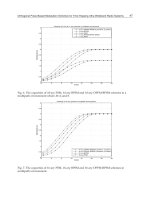
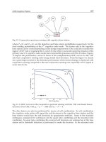
To show how Theorem 5 works, we give a simple example using QCC sequences,
where
11p  and 11L

. Fig. 6 and Fig. 7 show the distributions of correlation function
values of QCC sequences when 11N

and 21N

, respectively. By comparing two
figures, we can see that the maximum TH correlation function values are deceased to a half
of original values.



-60 -40 -20 0 20 40 60
0
5
10
15
Correlation Function Values
shift
-60 -40 -20 0 20 40 60
0
1

2
3
4
Correlation Function Values
shift
(a)
(b)


Fig. 6. The distribution of correlation function values of QCC sequences, where 11N  . (a).
ACF of


11
(2)
()k
c ; (b). CCF between


11
(3)
()k
c and


11
(5)
()k
c

Novel Applications of the UWB Technologies

112
-100 -50 0 50 100
0
5
10
15
Correlation Function Values
shift
-100 -50 0 50 100
0
0.5
1
1.5
2
Correlation Function Values
shift
(a)
(b)

Fig. 7. The distribution of correlation function values of QCC sequences, where 21N  . (a).
ACF of


11
(2)
()k
c ; (b). CCF between



11
(3)
()k
c and


11
(5)
()k
c
5. TH sequences with ZCZ
In this section, we begin with the definition of ZCZ of TH sequences to understand how
ZCZ works. We then construct a class of TH sequences with ZCZ and prove the correlation
properties of such TH sequences when the shifts between ZCZ TH sequences are in the
range of ZCZ.
5.1 Definition of ZCZ of TH sequences
According to Definition 3 on TH period correlation function, we can define the ZCZ of TH
sequences as follows.
Definition 5: Let C
ij
(l) denotes TH periodic correlation function between two TH sequences


()
()
L
i
k
c and



()
()
L
j
k
c with period L , and then ZCZ of TH sequences can be expressed as

Time-Hopping Correlation Property and Its Effects on THSS-UWB System

113

,0
()
0, 0 | |
2
ii
A
CZ
Ll
Cl
Z
l









(18)
and

() 0, 0 || ,
2
CCZ
ij
Z
Cl l i j

 
, (19)
where
A
CZ
Z and
CCZ
Z denote TH zero auto-correlation zone (ZACZ) width and TH zero
cross-correlation zone (ZCCZ) width, respectively.
According to definition 5, both of CCF and ACF sidelobes are equal to zero when the shifts
between TH sequences are in the range of
CZ
Z , where {,}
CZ ACZ CCZ
ZminZZ

. Then,
orthogonal communications can be realized when the approximate chip synchronization is

held between users in whole system.
5.2 Construction of ZCZ TH sequences
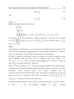
The principle of construction of ZCZ TH sequences can be depicted in Fig. 8, where




(1) (1)
() ()
LL
kk
ce
and




(2) (2)
() ()
1
LL
eh CCZ
kk
cNZe
respectively denote two TH sequences,
and


()
()

L
i
k
e is any existing TH sequence satisfying
()
()
0
L
i
eh
k
eN.


Fig. 8. The principle of construction of ZCZ TH sequences
According to Fig. 8,
(1) (1)
(0) (0)
2
LL
ce

 ,
(1) (1)
(1) (1)
0
LL
ce

 ,

(2)
(0)
1
L
e

, 3
eh
N

and 6
CCZ
Z  . Then,
we have
(2) (2)
(0) (0)
1316111
LL
eh CCZ
cN Ze  . In terms of such principle, a class of
ZCZ TH sequences can be constructed as follows.
Construction of ZCZ TH Sequences: For the given ZCZ width
CZ
Z which is determined by
THSS-UWB systems, a novel ZCZ TH sequence


()
()
L

i
k
c can be expressed as

() ()
() ()
(1)( 1 )
LL
ii
eh CZ
kk
ciN Ze   . (20)
The widths of ZACZ and ZCCZ satisfy
CCZ c
Z
T





(1)


f
ACZ eh c
TZ N T
(1)
eh c
NT


112
0

Novel Applications of the UWB Technologies

114
(1) 1 1
ACZ u eh CZ eh eh
ZNN ZN NN


and
CCZ CZ
ZZ ,
where
(1)
ueh CZ
NN N Z 
and
()
()
0
L
i
eh
k
eN.
Based on Definition 3, correlation properties of the constructed ZCZ TH sequences can be
proved as follows.

Proof: (1). We first consider the case of ij

, namely CCF.
Let the synchronization error

of a THSS-UWB system satisfy
||
2
CZ
c
Z
T



when the
approximate chip synchronization is held in the whole system. Correspondingly, the shift
between two TH sequences is equal to
laNb

 , where 0 1aL

 and
0
CZ
bZ
. The
evaluation of ( )
ij
Cl will be carried out in two steps on the basis of its two components.

i.
According to the equation (20), the first part of ( )
ij
Cl can be expressed as
11
() ()
() ()
() () () ()
00
[( ) ,( ) ] [(( )( 1 ) ( )) ,( ) ]
LL LL
LL
jj
i i
NL NL eh CZ NL NL
ka k ka k
kk
hc c b h i j N Z e e b

 

   

,
where
()
()
() ()
LL
j

i
eh eh
ka k
Ne e N

   since
()
()
()()
0,
LL
j
i
eh
ka k
eeN

. Then, it is obvious that
()
()
() ()
(( )( 1 ) ( )) 1
LL
j
i
eh CZ NL CZ
ka k
ijN Z e e Z

   when ij . If ij


, we will have
(1) 1
u
Nij
. Then,
()
()
() ()
(1)( 1 ) ()( 1 )( )
(1)
(1 )
0
LL
j
i
uehCZeh ehCZ
ka k
eh CZ eh
CZ
NN ZNijN Ze e
NZN
Z

     
   
 


We can further obtain that

() ()
() ()
( ) () ( ) ()
(( )( 1 ) ( )) |( )( 1 ) ( )|
(1)( 1 )
(1)(1)(1)
(1) ( 1)(1 )
1
LL LL
jj
ii
eh CZ NL eh CZ
ka k ka k
uehCZeh
ueh CZ u eh CZ eh
uehuu CZ
CZ
ijNZee NLijNZee
NL N N Z N
NN Z L N N Z N
NL N NLN Z
Z

   
   




As a result, when

ij

, we have
()
()
() ()
(( )( 1 ) ( )) 1
LL
j
i
eh CZ NL CZ
ka k
ijN Z e e Z

  .
Due to
0
CZ
bZ , we can obtain that

Time-Hopping Correlation Property and Its Effects on THSS-UWB System

115
11
() ()
() ()
() () () ()
00
[( ) ,( ) ] [(( )( 1 ) ( )) ,( ) ]
0

LL LL
LL
jj
i i
NL NL eh CZ NL NL
ka k ka k
kk
hc c b h i j N Z e e b

 

   



ii.
The second part of ( )
ij
Cl can be expressed as
1
()
()
(1) ()
0
1
()
()
(1) ()
0
[( ) ,( ) ]

[(( )( 1 ) ( )) ,( ) ]
LL
LL
L
j
i
NL NL
ka k
k
L
j
i
uehCZ NLNL
ka k
k
hN c c b
hN ijN Z e e b











Similarly, when
ij


, we can obtain that
()
()
(1) ()
(( )( 1 ) ( )) 1
LL
j
i
uehCZ NLCZ
ka k
NijN Z e e Z

       . Due to
0
CZ
bZ
, we can obtain
that
1
()
()
(1) ()
0
[( ) ,( ) ] 0
LL
L
j
i
NL NL

ka k
k
hN c c b





.
In terms of the above analyses, the CCF values of the constructed ZCZ TH sequences are
equal to zero when the shifts are in range of
CCZ
Z
, namely ( ) 0
ij
Cl

when
0
2
CCZ
Z
l

and
ij .
(2). Secondly, we consider the case of
ij

, namely ACF.

For an approximately synchronized THSS-UWB system, when multipath delay is in the
range of
ACZ c
ZT , the shift of TH sequence


()
()
L
i
k
c is correspondingly equal to laNb,
where 0a  and
0
A
CZ
bZ

 .
Similar to ( )
ij
Cl, the evaluation of
()
ii
Cl
will be carried out in two steps.
i.
According to equation (20), the first part of ()
ii
Cl can be expressed as

11
() ()
() ()
00
[(( )( 1 ) ( )) ,( ) ] [(0) ,( ) ]
LL
LL
ii
eh CZ NL NL NL NL
kk
kk
hiiN Z e e b h b


 

.
Due to
0
ACZ
bZ , we have
11
() ()
() ()
00
[( ),( )] [(0),()]0
LL
LL
ii
NL NL NL NL

ka k
kk
hc c b h b






.
ii.
The second part of ()
ii
Cl can be expressed as
1
() ()
(1) ()
0
1
() ()
(1) ()
0
[(( )( 1 ) ( )) ,( ) ]
[( ( 1 ) ( )) ,( ) ]
LL
LL
L
ii
uehCZ NLNL
kk

k
L
ii
ueh CZ NL NL
kk
k
hN iiN Z e e b
hN N Z e e b






    




Due to
() ()
(1) ()
LL
ii
eh eh
kk
Ne e N

   and
(1)

ueh CZ
NN N Z 
, we can obtain that
eh
NN

() ()
(1) ()
(1)( )
LL
ii
ueh CZ eh
kk
NN Z e e N N


. Also, since
01
SCZ eh
bZ NN

, then,

Novel Applications of the UWB Technologies

116
11
()
() () ()
(1) () (1) ()

00
[( ) ,( ) ] [( ( 1 ) ( )) ,( ) ]
0
LL LL
LL
j
i ii
NL NL u eh CZ NL NL
ka k k k
kk
hN c c b hN N Z e e b

 





According to the above analyses, the ACF sidelobes of the constructed ZCZ TH sequences
are equal to zero when the shifts are in range of
A
CZ
Z .
Q.E.D.
6. Effects of TH correlation properties on MAI in THSS-UWB systems
By transforming the signal model of THSS-UWB communication systems, we obtain
expressions for the relation of MAI values and TH correlation function values in this
section,.
6.1 Binary model of TH sequences
According to the equation (1), we can see that only one pulse is transmitted to each user

within any frame time
f
T , i. e. One-Pulse-Per-Frame structure (Erseghe, 2002b; Scholtz et al,
2001). The pulse position is decided by TH sequence


()
()
L
i
k
c , namely
()
()
.
L
i
c
k
cT
. For more
easiness to understand, the structure is depicted in Fig. 9, where elements of a TH sequence
are binary ones.


Fig. 9. The hopping format of pulses in PPM
We assume that “1” denotes the time slot where a pulse is modulated, and the other time
slots in frame time
f
T are “0”. As a result, the binary TH sequence



()
()
NL
i
n
a
can be obtained.
The sequence


()
()
NL
i
n
a corresponds to


()
()
L
i
k
c and its period is equal to NL . According to the
above analyses, the equation (1) may be transformed as

() ()
()

() [/( )]
() ( )
NL s
ii
i
c
nnNN
n
St a wtnT d






, (21)
()
()
NL
i
n
a
1 0 0 0 0 0 1 0 0 0 0 1 0 1 0 0
f
T
c
T
()
(3)
1

L
i
c

()
(2)
3
L
i
c

()
(1)
2
L
i
c


Time-Hopping Correlation Property and Its Effects on THSS-UWB System

117
where

()
()
()
()
1, int
0,

L
NL
i
i
k
n
nkNc
f
or some e
g
er k
a
otherwise







.
Then, the TH periodic correlation function between


()
()
L
i
k
c and



()
()
L
j
k
c in Definition 3 can be
also expressed as

1
()
()
() ( )
0
()
NL NL
LN
j
i
ij
nnl
n
Cl a a





, (22)

where l denotes the shift between


()
()
NL
i
n
a
and


()
()
NL
j
n
a
, 0 1lNL

.
Note that the equation (22) is different from the periodic correlation function of DSs. The
correlation function of binary TH sequences describes the number of agreements to element
“1” between sequences, called the number of collisions, where
()
()
NL
i
n
a is equal to “0” or “1”

instead of “
1 ” and “ 1

” in ordinary correlation function, such as in DS systems. In other
words, if both of
()
()
NL
i
n
a and
()
()
NL
j
n
a are “1” in some time slot where user i and user
j
collide,
then their multiplication
()
()
() ()
.
NL NL
j
i
nn
aa will be also “1”.
As a result, the binary TH correlation function in the equation (22) refers to the number of

collisions. The smaller C
ij
(l) gets, the smaller the number of collisions are, and the better TH
correlation properties are.
6.2 Multiple-access performance
In THSS-UWB multiple-access communication systems, when
u
N links are active, the
received signal
()rt may be expressed as follows (Scholtz, 1993),

()
1
() ( ) ()
u
N
i
ii
i
rt AS t nt




, (23)
where
i
A represents the attenuation of transmitter k’s signal over the propagation path to
the receiver, and
i


denotes time asynchronisms between the clocks of transmitter k and
the receiver. The notation
()nt is white Gaussian receiver noise.
Without loss of generality, we assume that the receiver is interested in determining the data
sent by transmitter 1 in the following analyses. We also assume that one data symbol is
modulated by
L pulses, i. e.
S
NL

, and the correlation demodulation is employed. When
symbol “0” is sent, the shift time is zero, and the shift time is

when symbol “1” is sent.
Then, a template signal can be given by

1
()
()
(1)
() [ ( ) ( )]
s
NL
s
kN N
i
cc
n
nk NN

Vt a wt nT wt nT


 


(24)
For transmitter 1, the demodulation output of the k
th
bit is

Novel Applications of the UWB Technologies

118

(1)
(1)
() ()
sc
sc
kN NT
k
kNNT
TrtVtdt

 


. (25)
Then, the received bit is decided as “0” when

(1)
0
k
T  . Obviously, when
(1)
0
k
T  , the
received bit is determined as “1”.
The equation (25) is also described as
(1)
()
()
1
(1)
*
111
(1)
2
(1) [ ( )(1) ( )(1) ] () ()
u
i
i
sc
kmm
sc
N
kN NT
d
d

d
sPiii ii P
k
kNNT
i
TAN E AR R E ntVtdt



 

    


,
(26)
where
()[ () ( )]
P
Ewtwtwtdt





,
()i
m
d and
()

1
i
m
d

represent the
th
m bit and ( 1)
th
m  bit
of user i , respectively. Transmitter 1 sends the
th
k bit.
1
()
ii
R

and
*
1
()
ii
R

denote the TH
part correlation function between user i and user 1 in continuous time, respectively,
namely
()
()

0
()
j
i
ij t t
Raadt






and
()
()
*
()
c
LNT
j
i
ij t t
Raadt








.
It is obvious that
*
() () ()
ij ij ij
RRY


, where ( )
ij
Y

is continuous TH period correlation
function in Definition 4.
In the equation (26), the first part is the signal that we desire. The second part represents the
MAI that the other users make to user 1, and the last part is the interference made by noise.
We are interested in the second part, which will be analyzed in the following. The analysis
of THSS-UWB MAI is similar to the performance evaluation for DSSS multiple-access
communications (Pursley, 1977).
In order to analyze the second part of equation (26), we define now the TH aperiodic
correlation function in discrete time as follows,

1
()
()
() ( )
0
1
()
()

() ()
0
,0 1
() , 1 0
0,
NL NL
NL NL
LN l
j
i
nnl
n
LN l
j
i
ij
nl n
n
aa lLN
Zl a a LN l
lLN








  
















. (27)
According to the equation (27), in the range of
0(1)
ccc
lT l T L N T


   , ( )
ij
R

and
*
1
()

ii
R

can be expressed as ()()[(1)()]()
i
j
i
j
ci
j
i
j
c
R Zl LNT Zl LN Zl LN lT



       
and
*
( ) () [ ( 1) ()]( )
i
j
i
j
ci
j
i
j
c

RZlTZlZl lT

 , respectively.
Meanwhile, the TH period correlation function ( )
ij
Cl in the equation (22) can be expressed
as ( ) ( ) ( ),
ij ij ij
Cl Zl Zl LNand TH period odd correlation function can be also defined as
*
() () ( )
ij ij ij
Cl Zl ZlLN.
From the equation (26), the interference made by user i with user 1 satisfies
()
()
1
*
11 1
() [ ()(1) ()(1) ]
i
i
mm
d
d
ii i ii ii P
M
AR R E
 



.
Let
(1)
ic i i c
lT l T

. When
()
()
1
i
i
m
m
dd

 , we have

Time-Hopping Correlation Property and Its Effects on THSS-UWB System

119

()
()
()
*
111
111 1
11

111
() [ () ()](1)
{[ ( ) ( )] [( ( 1 ) ( 1))
( ( ) ( ))] ( )} ( 1)
{() [( 1) ()]( )}(1)
i
m
i
m
i
m
d
ii iii ii P
i ii ii c ii ii
d
ii ii i ic P
d
iii c ii ii i ic
MARR E
AZl LN Zl T Zl LN Zl
Zl LN Zl lT E
AClT Cl Cl lT E




    
 

P

(28)
Similarly, when
()
()
1
i
i
m
m
dd

 , we have

()
()
*
111
***
111
() [ () ()](1)
{() [( 1) ()]( )}(1)
i
m
i
m
d
ii iii ii P
d
iii c ii ii i ic P
MARR E

AClT Cl Cl lT E




     
(29)
The equations (28)-(29) provide the desired relation between multiple-access interference
1
()
ii
M

and TH correlation function ( )
ij
Cl (or
*
()
ij
Cl).
Note that
11 1
[ ( 1) ( )]( ) ( )
ii ii i ic iic
Cl Cl lT ClT


 and
** *
11 1

[( 1) ()]( ) ()
ii ii i ic iic
Cl Cl lT ClT

    . Hence, the equations (28)-(29) can be respectively
expressed as
()
11
() () (1)
i
m
d
ii iii c P
M
AC l T E


 for
()
()
1
i
i
m
m
dd

 and
()
*

11
() () (1)
i
m
d
ii iii c P
M
AC l T E

 for
()
()
1
i
i
m
m
dd

 . They describe the interference to user1 from
user i . Furthermore, we consider a more general situation, where
u
N users are active.
Since ( ) ( ) ( )
ij ij ij
Cl Zl Zl LN and
*
() () ( )
ij ij ij
Cl Zl ZlLN


, then
1max
()
ii
Cl C
and
*
max 1 max
()
ii
CClC  . Hence, we consider the worst scenario, which happens when
1max
()
ii
Cl C
and
*
1max
()
ii
Cl C . Let
SIR
I
denote signal-to-interference ratio (SIR) which
describes the interference to user 1 from the other
1
u
N


users and thermal noise, then

2
1
22
11
2
()
u
SIR
N
ii
i
D
I
NM





, (30)
where
()
1max
() (1)
i
m
d
ii i c P

M
AC T E


,
(1)
11
(1)
k
d
s
p
DAN E

 , and
1
(1)
() ()
sc
sc
kN NT
kNNT
NntVtdt

 


. Then,
SIR
I can be expressed as

22
2
max
2
1
2
1
1
()
u
SIR
N
ci
SNR
i
s
I
CT A
IA
N





, (31)
where
2
1

2
1
SNR
D
I
N

, which is a convenient parameter and equivalent to the output signal-to-
noise (SNR) ratio that one might observe in single link experiments.
Then, the BER can be given by

2
1
exp( / 2)
2
SIR
e
I
Pxdx




. (32)

Novel Applications of the UWB Technologies

120
According to the equations (30)-(33), we can see that the interference and the BER are
determined by

max
C when
1
A ,
i
A ,
s
N ,
c
T and
SNR
I are specific. For the construction of TH
sequences in THSS-UWB communication systems, TH correlation function values should be
as small as possible so that the multiple access interference and the probability of error are
small.
Similarly, for another hoping format in THSS-UWB, called PAM, the relation between
multiple-access interference
1
()
ii
M

and TH correlation function ( )
ij
Cl (or
*
()
ij
Cl) may be
respectively given as

()
1111
() { () [ ( 1) ()]( )}
i
ii im ii c ii ii iic P
M
Ad C l T C l C l lT E


     for
()
()
1
i
i
m
m
dd

 and
()
***
1111
() { () [ ( 1) ()]( )}
i
ii im ii c ii ii iic P
M
Ad C l T C l C l lT E



     for
()
()
1
i
i
m
m
dd

 , where the data
()i
m
d is a binary stream (“ 1

”or “ 1

”) instead of “0” or “1” in
PPM format.
7. Conclusion
The main intention of this chapter is to analyze the correlation properties of TH sequences
for THSS-UWB systems. A more general definition of TH periodic correlation function is
provided and the definition can be used to analytically evaluate the TH correlation
properties in codeword synchronism, chip synchronism and asynchronism in the whole
system. Based on the definition, theoretical bounds of TH sequences are presented, which
relate four parameters of
L , N ,
u
N and
max

C (or
max
S ). The results can be used to
evaluate the performance of TH sequences and provide references for the design of TH
sequences. Also, based on the definition, a method to improve TH correlation properties in
practical applications is proposed. The maximum correlation function values of TH
sequences can be reduced to a half of original values by such a method. Specially, in terms
of this method, the maximum correlation function values of QCC sequences can be reduced
from
max
2S  and
max
4C

to
max
1S

and
max
2C

, which achieves the best TH
correlation properties so far in an asynchronized THSS-UWB system.
A novel TH sequence family with TH ZCZ for approximately synchronized THSS-UWB
systems is constructed and its correlation properties are proved in terms of the definition of
TH periodic correlation function presented in this chapter. When the approximate chip
synchronization is held in the whole system, the MAI of THSS-UWB system employing the
proposed ZCZ TH sequences is eliminated, and such THSS-UWB systems are more tolerant
to the multipath problem. As a result, orthogonal communications can be realized while the

need of accurate synchronism in whole system is reduced.
In addition, the multiple access performance is investigated and the relation between MAI
values
SIR
I and TH correlation function values
max
C are formulated by transforming the
signal model from decimal sequence


()
()
L
i
k
c to binary sequence


()
()
NL
i
n
a . Based on the
obtained results, TH correlation function values should be as small as possible so that the
multiple access interference and the probability of error are small.
8. Acknowledgement
We thank the National Natural Science Foundation of China (NSFC) under Grant no.
61002034 and 60872164, the Natural Science Foundation Project of CQ CSTC under Grant

Time-Hopping Correlation Property and Its Effects on THSS-UWB System

121
no. 2009BA2063 and 2010BB2203, Chongqing University Postgraduates’ Innovative Team
Building Project under Grant no. 200909B1010, and Open Research Fundation of Chongqing
Key Laboratory of Signal and Information Processing (CQKLS&IP) under Grant no. CQSIP-
2010-01 for supporting this work.
9. References
Canadeo, C.M., Temple, M.A., Boldwin, R.O. & Raines, R.A., (2003). UWB Multiple Access
Performance in Synchronous and Asynchronous Networks, Electron. Lett., Vol.39,
No. 11, May 2003, pp. 880-882.
Corrada-Bravo, C., Scholtz, R. A. & Kumar, P. V., (1999). Generating TH-SSMA Sequences
with Good Correlation and Approximately Flat PSD Level, Proceedings of UWB’99,
Sept. 28, 1999.
Chu, W. S.& Colbourn, C.J., (2004). Sequence Designs for Ultra-Wideband Impulse Radio
with Optimal Correlation Properties, IEEE Trans. Inf. Theory, Vol. 50, No. 10, Oct.
2004, pp. 2402-2407.
Durisi, G. & Benedetto, S., (2003). Performance Evaluation of TH-PPM UWB Systems in the
Presence of Multiuser Interference, IEEE Commun. Letters, Vol. 7, No.5, May 2003,
pp. 224-226.
Erseghe, T., (2002). Ultra Wide Band Pulse Communications, Ph.D. thesis, Universita’ di
Padova, Italy, Feb., 2002.
Erseghe, T., (2002). Time-Hopping Patterns Derived from Permutation Sequences for Ultra
Wide Band Impulse Radio Applications, Proceedings of 6th WSEAS International
Conf. on Communications, July 7-14, 2002, pp.109-115.
Erseghe, T. & Bramante, N., (2002). Pseudo-Chaotic Encoding Applied to Ultra-Wide-Band
Impulse Radio, Proceedings of VTC’04F, Vol. 3, Vancouver, Canada , Dec., 2002, pp.
1711-1715.
Fan, P. Z., Suehiro, N., Kuroyanagi, N. & Deng, X. M., (1999). Class of Binary Sequences
with Zero Correlation Zone, Electron. Lett., Vol. 35, No. 10, Oct. 1999, pp. 777-779.

Gao, J. & Chang, Y. (2006). New Upper Bounds for Impulse Radio Sequences, IEEE Trans.
Inf. Theory, Vol. 52, No. 5, May 2010, pp. 2255-2260.
Guvene, I. & Arslan, H., (2004). TH-Sequences Construction for Centralised UWB-IR
Systems in Dispersive Channels, Electron. Lett., Vol. 40, No. 8, April 2004, pp. 491-
492.
Guvene, I. & Arslan, H., (2004). Design and Performance Analysis of TH Sequences for
UWB-IR Systems, Proceedings of WCNC’04, Atlanta, GA, USA, 2004, pp. 914-919.
Hayashi, T., (2009). A Class of Zero-Correlation Zone Sequence Set Using a Perfect
Sequence, IEEE Signal Process. Lett., Vol. 16, No.4, April 2009, pp. 331-334.
Hu, B. & Beaulieu, N. C., (2003). Exact Bit Error Rate Analysis of TH-PPM UWB Systems in
the Presence of Multiple-Access Interference, IEEE Commun. Letters, Vol. 7, No. 12,
Dec. 2003, pp. 572-574.
Hu, H. G. & Gong, G., (2010). New Sets of Zero or Low Correlation Zone Sequences via
Interleaving Techniques, IEEE Trans. Inf. Theory, Vol. 56, No. 4, April 2010, pp.
1702-1713.
Iacobucci, M.S. & Di Benedetto, M.G., (2001). Time Hopping Codes in Impulse Radio
Multiple Access Communication Systems, Proceedings of International Symposium on
third generation Infrastructure and services, Athens, Greece, 2-3 July 2001.

Novel Applications of the UWB Technologies

122
Iacobucci, M.S. & Di Benedetto, M.G., (2002). Multiple Access Design for Impulse Radio
Communication Systems, Proceedings of ICC’02, Vol. 2, Aug., 2002, pp. 817-820.
Le Martret, C. J. & Giannakis, G. B. (2000). All-Digital PAM Impulse Radio for Multiple-
Access through Frequency-Selective Multipath, Proceedings of GLOBELCOM’00,
Vol. 1, San Francisco, USA, 27 Nov. - 1 Dec. 2000, pp. 77-81.
Maggio, G.M., Rulkov, N., Sushchilk, M., Tsmring, L., Volkovskii, A., Abarbanel, H., Larson,
L. & Yao, K., (1999). Chaotic Pulse Position Modulation for UltraWide-Band
Communation System, Proceedings of UWB ‘99, Sept., 1999, pp.28-30.

Maggio, G.M., Rulkov, N. & Reggiani, L., (2001). Pseudo-Chaotic Time Hopping for UWB
Impulse Radio, IEEE Trans. on Circuits and Systems-I, Vol 48, No. 12, Dec., 2001, pp.
1424-1435.
Mireles, F. R., (2001). Performance of Ultrawideband SSMA Using Time Hopping and M-ary
PPM, IEEE J. Sel. Areas Commun., Vol. 19, No. 6, June 2001, pp. 1186-1196.
Pursley, M. B., (1977). Performance Evaluation for Phase-Coded Spread-Spectrum Multiple
Access Communication—Part I: System Analysis, IEEE Trans. Commun., Vol. 25,
No.8, Aug. 1977, pp. 795-799.
Scholtz, R. A. (1993). Multiple Access with Time Hopping Impulse Modulation, Proceedings
of MILCOM ‘93, Bedford, MA, USA, Oct. 11-14, 1993, pp. 447-450.
Scholtz, R. A., Kumar, P. V. & Bravo, C. C., “Some Problems and Results in Ultra-WideBand
Signal Design, Proceedings of SETA’01, May, 2001.
Suehiro, N., (1992). Elimination Filter for Co-Channel Interference in Asynchronous SSMA
Systems Using Ployphase Modulatable Orthogonal Sequences, IEICE Trans.
Commun., Vol. E75-B, June 1992.
Suehiro, N., (1994). A Signal Design without Co-Channel Interference for Approximately
synchronized CDMA System, IEEE J. Sel. Areas Commun., SAC-12, June 1994, pp.
837-841.
Sushchick, M. Jr., Rulkov, N., Tsimring, L., Abarbanel, H., Yao, K. & Volkovskii, A., (2000)
Chaotic Pulse Position Modulation: A Robust Method of Communicating with
Chaos, IEEE Commun. Letters, Vol. 4, No. 4, April, 2000, pp. 128-130.
Titlebaum. E. L., (1981). Time-Frequency Hop Signals, Part I: Coding Based upon the Theory
of Linear Congruences, IEEE Trans. on Aerospace and Elect. Syst., Vol.17, No.4, July
1981, pp. 490-493.
Win, M. Z. & Scholtz R. A. (1998). Impulse Radio: How It Works, IEEE Commun. Letters,
Vol.2, No.2, Feb. 1998, pp. 36-38.
Win, M. Z. & Scholtz R. A. (2000). Ultra-Wide Band-Width Time-Hopping Spread-Spectrum
Impulse Radio for Wireless Multiple-Access Communications, IEEE Trans. on
Commun., Vol. 48, No. 4, April 2000, pp. 679-690.
Zeng, Q. Peng, D. Y. & Wang, X. N., (2011). Performance of a Novel MFSK/FHMA System

Employing No-Hit Zone Sequence Set over Rayleigh Fading Channel, IEICE Trans.
Fundamentals, Vol. E94-A, No. 2, Feb. 2011, pp. 526–532.
Zhao, L. & Haimovich, A. M., (2002). The Capacity of an UWB Multiple-Access
Communications System, Proceedings of ICC’02, Vol.3, 2002, pp.1964-1968.
6
Fine Synchronization in UWB
Ad-Hoc Environments
Moez Hizem and Ridha Bouallegue
6’Tel/Sup’Com, University of Carthage
Tunisia
1. Introduction
UWB impulse radios (UWB-IR) have attracted increasing interest due to their potential to
propose high user capacity with low-complexity and low-power transceivers (Win & Sholtz,
2000). It is approved by the Federal Communications Commission’s (FCC) Report in which
the UWB spectral mask is released and published in February 2002. Most of these benefits
initiate from the distinctive characteristics inherent to UWB wireless transmissions (Yang &
Giannakis, 2004). These make UWB connectivity appropriate for indoor and especially
short-range high-rate wireless environments, as well as for strategic outdoor
communications. However, to harness these benefits, one of the most critical challenges is
the synchronization step and more specifically timing offset estimation. Bit error rate (BER)
analysis also exposes evident performance degradation of UWB radios due to mistiming
(Tian & Giannakis, 2005). The complexity of which is accentuated in UWB owing to the fact
that information bearing waveforms are impulse-like and have low amplitude. In addition,
compared to narrowband systems, the difficulty of timing UWB signals is increased further
by the dense multipath channel that remains unknown at the synchronization step. These
reasons give explanation why synchronization has obtained so much importance in UWB
research (Fleming et al, 2002; Homier & Sholtz, 2002; Tian & Giannakis, 2003; Yang et al,
2003).
Typically, pulse position modulation (PPM), pulse amplitude modulation or on/off keying
(OOK) is employed. PPM modulation transmits pulses with constant amplitude and encodes

the information according to the position of the pulse, while PAM and OOK use the amplitude
for this purpose. Moreover, PPM is regularly implemented to reduce transceiver complexity in
UWB systems. But unlike pulse amplitude modulation (PAM) applied in the context of UWB
systems, the difficulty of accurate synchronization is accentuated in PPM UWB systems owing
to the fact that information is transmitted by the shifts of the pulse positions.
In the last years, numerous timing algorithms have been studied for UWB impulse radios
under various operating environments. Least squares (LS) (Carbonelli et al, 2003) and
Maximum-likelihood (ML) approaches (Lottici et al, 2002) are available, but tend to be
computationally complex as they need high sampling rates. In (Djapic et al, 2006), a blind
synchronization algorithm that takes advantage of the shift invariance structure in the
frequency domain is proposed. An accurate signal processing model for a Transmit-
reference UWB (TR-UWB) system is given in (Dang et al, 2006). The model considers the

Novel Applications of the UWB Technologies
124
channel correlation coefficients that can be estimated blindly. In (Ying et al, 2008), the
authors proposed a code-assisted blind synchronization (CABS) algorithm which relies on
the discriminative nature of both the time hopping code and a well-designed polarity code.
Timing with dirty templates (TDT), which is the starting point of this paper, was introduced
in (Yang & Giannakis, 2005) for rapid synchronization of UWB signals and was developed
in (Yang, 2006) for PPM-UWB signals with direct sequence (DS) and/or time hopping (TH)
spreading. This technique is based on correlating adjacent symbol-long segments of the
received waveform. TDT is functional with random and unknown transmitted symbol
sequences. When training symbols are approachable, the performance of the TDT
synchronizer can be improved by approving a data-aided (DA) mode (Yang & Giannakis,
2005). The DA mode significantly outperforms the non-data-aided (NDA) one. However, the
training sequences require an overhead which reduces the bandwidth and energy efficiency.
Except (Yang, 2006), all these timing algorithms are developed for PAM-UWB signals. Since
their operations greatly rely on zero-mean property of PAM, these presented timing
algorithms are not appropriate to PPM-UWB signals.

In this chapter, to address and try to solve the problem of synchronization for Ultra
Wideband (UWB) systems in ad-hoc environments, we propose a fine synchronization
algorithm for PAM and PPM UWB signals with a spread spectrum involving Time Hopping
(TH). We adopt first a blind (or coarse) synchronization technique, which is Timing with
dirty templates (TDT). Its principle is to correlate two consecutive symbol-long segments of
the received waveform. In particular, synchronization will be asserted when the correlation
function reaches its maximum. This allows TDT algorithms to effectively collect the
multipath energy even when the spreading codes and the channel are both unknown.
However, this technique estimates coarsely (or roughly) the value of timing offset, therefore
not precisely, and this may cause a shortfall in performance of our UWB impulse radio
systems. To improve synchronization performance of the TDT (Timing with Dirty
Templates) algorithm developed in mentioned papers, our contribution will be to
implement a new fine synchronization stage and place it after the dirty one, which is TDT
approach. The principle of our fine synchronization algorithm is to make a fine research in
order to find the exact moment of the beginning pulse (fine estimation of delay time
between emitted pulses and those received). This is achieved by correlating two consecutive
segments of symbol-length received waveform, but this time in an interval that corresponds
to the number of frames included in one data symbol. First, we applied this algorithm in
single-user environments and then, have extended the used method in multi-user
environments. Simulation results show that this new approach using TDT synchronizer can
achieve a lower mean square error (MSE) than the original TDT for both NDA and DA
synchronization mode.
The rest of this chapter is organized as follows. We describe our system model (PAM and
PPM signals through time hopping spreading) with first stage synchronization (based on
TDT) in Section 2, and then we give an outline of the well known TDT approach for UWB
TH-PAM and TH-PPM impulse radios to better understand the overall timing
synchronization in Section 3. In Section 4, we present the second step or stage of our
synchronization approach with UWB time hopping systems in ad-hoc environments. The
performance evaluation of our proposed fine synchronization approach with UWB TH-
PAM and TH-PPM impulse radio systems in both single-user and multi-user environments

is given in Section 5. And finally, we conclude this chapter in Section 6.

Fine Synchronization in UWB Ad-Hoc Environments
125
2. TH-PAM and TH-PPM UWB system model
Common multiple access techniques implemented for pulse based UWB systems are Time
Hopping (TH) and Direct Sequence (DS). Appropriate modulation techniques include OOK
(Foerster et al, 2001) and particularly PPM and PAM (Hämäläinen et al, 2002). A given
UWB communication system will be a mixture of these techniques, leading to signals based
on, for example, TH-PPM, TH-BPAM or DS-BPAM. TH-PAM and TH-PPM are almost
certainly the most frequently adopted scheme and will be applied in the following as an
example for determining the resources existing in a UWB system in single-user and multi-
user environments.
2.1 TH-PAM UWB system model for single-user links
In UWB impulse radios, each information symbol is transmitted over a T
s
period that
consists of N
f
frames (Win & Sholtz, 2000). During each frame of duration T
f
, a data-
modulated ultra-short pulse p(t) with duration 

≪

is transmitted from the antenna
source. The transmitted signal is
v
(

t
)
=
√
ε
∑
s


(
k
)∑
p
(
t−iT

−c

(
i
)
T

−kT

)





(1)
where ε is the energy per pulse. ̃
(

)
≔()̃
(
−1
)
are differentially encoded symbols and
drawn equiprobably from a finite alphabet. In our case, s(k) are denoting the binary PAM
information symbols. User separation is realized with pseudo-random TH-codes c
th
(i),
which time-shift the pulse positions at multiples of the chip duration T
c
(Win & Sholtz,
2000). In this paper, we focus on a single user link and treat multi-user interference (MUI) as
noise.
The transmitted signal propagates through the multipath channel with impulse response
g
(
t
)
=
∑
α

δ(t−τ


)


(2)
where
{


}


and
{


}


are amplitudes and delays of the L multipath elements,
respectively. The channel is assumed quasi-static and among
{


}


, τ
0
represents the
propagation delay of the channel.

Then, the received waveform is given by
r
(
t
)
=
√
ε
∑
s
(
k
)
p

t−kT

−τ
,
−τ

+η(t)


 (3)
where 
,
is arbitrary reference at the receiver representing the delay relative to the arrival
moment of the first pulse, () is the additive noise and 


() denotes the received symbol
waveform as
p

(
t
)
=
∑
p
(
t−iT

−c

(
i
)
T

)




∗g
(
t+τ

)

 (4)
where * indicates the convolution operation. We define the timing offset as ∆≔ 
,
−

.
Let us suppose that ∆ is in the range of [0, T
s
) and we will show in the rest of this paper that
this assumption will not affect the timing synchronization.
2.2 TH-PPM UWB system model for single-user links
With PPM modulation (Durisi & Benedetto, 2003; Di Renzo et al, 2005), the transmitted
signal in single-user links is described by the following model

Novel Applications of the UWB Technologies
126
v
(
t
)
=
√
ε
∑∑
p
(
t−iT

−c


(
i
)
T

−kT

−d

δ
)







(5)
where ε is the energy per pulse, d

∈(0,1) represents the i-th information bit transmitted,
and δ is the time shift associated with binary PPM. User separation is realized with pseudo-
random TH-codes c
th
(i), which time-shift the pulse positions at multiples of the chip
duration T
c
(Win & Sholtz, 2000). In this paper, we focus on a single user link and treat
multi-user interference (MUI) as noise.

After the transmitted signal propagation through the multipath channel, the received
waveform is given by
r
(
t
)
=
√
ε
∑
α



∑
p

t−kT

−τ
,
−τ

−d

δ+η
(
t
)



(6)
where τ
,
is arbitrary reference at the receiver representing the delay relative to the arrival
moment of the first pulse, η(t) is the additive noise and p

(t) denotes the received symbol
waveform as
p

(
t
)
=
∑
p
(
t−iT

−c

(
i
)
T

)





∗g
(
t+τ

)
(7)
where * indicates the convolution operation. We define the timing offset as ∆τ ≔ τ
,
−τ

.
Let us suppose that ∆τ is in the range of [0, T
s
) and we will show in the rest of this paper that
this assumption will not affect the timing synchronization. Let p
R
(t) the overall received
symbol-long waveform defined as follows
p

(
t
)
=
∑
α

p


t−τ
,



 (8)
Using (8), the received waveform in (6) becomes
r
(
t
)
=
√
ε
∑
p

(
t−kT

−τ

−d

δ
)
+η(t)



(9)
2.3 TH-PAM UWB system model for single-user links
The UWB time hopping impulse radio signal considered in this paper is a stream of narrow
pulses, which are shifted in amplitude modulated (PAM). The transmitted waveform from
the uth user is
v

(t)=

ε

∑
s

(
k
)
p
,
(
t−kT

)


(10)
where ε

represents the energy per pulse, s


(
k
)
are differentially encoded symbols and
drawn equiprobably from finite alphabet. In our case, s

(
k
)
symbolize the binary PAM
information symbols and p
,
(t) indicates the transmitted symbol
p
,
(
t
)
:=
∑
p(t−iT

−c

(i)T

)





 (11)
where T

is the chip duration and c

(i) is the user-specific pseudo-random TH code during
the ith frame.
After the transmitted signal propagation through the multipath channel, the received
waveform from all users is
p
,
(
t
)
:=
∑
p(t−iT

−c

(i)T

)




 (12)
where N

u
is the user’s number, 

is the propagation delay of the uth user’s direct path and
() is the zero-mean additive Gaussian noise (AGN). The global received symbol-long
waveform is therefore given by

Fine Synchronization in UWB Ad-Hoc Environments
127
p
,
(
t
)
:=
∑
α
,
p
,
(t−τ
,
)




(13)
Assuming that the nonzero support of waveform 
,

(

)
is upper bounded by the symbol
time T
s
, the received waveform in (3) can be rewritten as
r
(
t
)
=
∑

ε

∑
s

(k)p
,
(
t−kT

−τ

)







+η
(
t
)
(14)
3. TDT approach
As mentioned previously, our proposed timing scheme consists of two complementary
floors or steps. The first is based on a coarse (or blind) synchronization that is TDT
developed in (Yang & Giannakis, 2005). In this section, we will give an outline of the TDT
approach to better understand the overall timing synchronization suggested in this paper.
The general structure description of our system model with first stage synchronization
(TDT) is illustrated in Fig.1.


Fig. 1. Description of our model with first stage synchronization
The basic idea behind TDT is to find the maximum of square correlation between pairs of
successive symbol-long segments. These symbol-long segments are called “dirty templates”
because: i) they are noisy, ii) they are distorted by the unknown channel, and iii) they are
subject to the unknown offset

. Then, we will analyze 

 representing estimate offset of 


by deriving upper bounds on their mean square error (MSE) in both non-data-aided (NDA)
and data-aided (DA) modes.

3.1 TDT approach for TH-PAM UWB system in single-user links
For notational brevity and after setting p
T
(t) := p
R
(t-τ
l,0
), the received waveform simplifies to
r
(
t
)
=
√
ε
∑
s


(
k
)
p

(t−kT

−τ

)+η(t) (15)
Thereafter, a correlation between the two adjacent symbol-long segments 

(
+

)
and

(
+(−1)

)
is achieved. Let (;) the value of this correlation∀∈
[
1,+∞
)
and
∈[0,

)

Novel Applications of the UWB Technologies
128
x(k;τ)=

r
(
t+kT

+τ
)




r
(
t+
(
k−1
)
T

+τ
)
dt (16)
Applying the Cauchy-Schwartz inequality and substituting the expressions of 
(
+

)

and 
(
+(−1)

)
to (16), (;) becomes
x(k;τ)=s(k−1)[s(k−2)ε

(τ

)+s(k)ε


(τ

)]+ζ(k;τ) (17)
where 

(

)
≔









(

)
, 

(

)
≔









(

)
, and (;) corresponds to the
superposition of three noise terms (Yang & Giannakis, 2005) and can be approximated as an
additive white Gaussian noise (AWGN) with zero mean and 

power.
By exploiting the statistical properties of the signal and noise, the mean square of the
samples in (17) is given by
E{x

(k;τ)}=


[ε

(τ

)+ε

(τ

)]2+



[ε

(τ

)−ε

(τ

)]2+σ


(18)
We notice that ε
B
(τ

)
+
ε
A
(τ

) = ε

p


(

t
)



dt := ε
R
for 

∈[0,

), where ε
R
represents the
constant energy corresponding to the unknown aggregate template at the receiver. Then the
mean square of x
2
(k;τ) can be rewritten as follows
E
{
x

(
k;τ
)
}
=




(
ε

)

+



[
2ε

(



)
−ε

]
2+


(19)
Since the term ε
A
(

) reaches its unique maximum at 


=0, then E{x
2
(k;τ)} also reached its
unique maximum at 

=0. Thus, an estimate of timing offset 

is given by
̂

=arg
∈
[
,

]
E{x

(k;τ)} (20)
In the practice, the mean square of x
2
(k;τ) is estimated from the average of different values
x
2
(k;τ) for k ranging from 0 to M – 1 obtained during an observation interval of duration MT
s
.
In what follows, we summarize the TDT algorithm in its NDA form and then in its DA form.
3.1.1 Non-data-aided (blind) mode
For the synchronization mode NDA, the synchronization algorithm is defined as follows


̂
,
=arg
∈
[
,

]
E{x

(k;τ)}
x

(
M;τ
)
=


∑


r
(
t+τ
)
r
(
t+τ+T


)
dt
()







 (21)
By using (17), the expression of 

(
;
)
can be rewritten as follows
x

(
M;τ
)
=


∑
[
s
(

m−1
)
s
(
m−2
)
ε

(



)
s
(
m
)
s
(
m−1
)
ε

(
τ


)
+ζ(m;τ)
]




(22)
From (19) and (20), the estimation of delay τ
0
is made possible due to the presence of the
term ε
A
(τ

) - ε
B
(τ

). Unfortunately for the estimator x

(
M;τ
)
, this term exists only if the
transmitted sequence presents an alternating sign between the symbols s
(
m−2
)
and s(m).
Thus, for the synchronization in NDA mode, the performances of this approach are affected
by the sign of the transmitted symbols. To increase the chances that the estimator x

(

M;τ
)

is expressed as a function of the energy difference, an increase in the observation interval
length is required. However, such an increase leads to increased acquisition delays. Where
does the idea of using the data-aided (DA) approach.

Fine Synchronization in UWB Ad-Hoc Environments
129
3.1.2 Data-aided mode
The number of samples M required for reliable estimation can be reduced noticeably if a
data-aided (DA) approach is pursued (Yang & Giannakis, 2003). The delays can be
significantly reduced through the use of training sequences with alternating sign between
the symbols s
(
m−2
)
and s(m), i.e. s(m – 2) = - s(m). This observation suggest that the
training sequence {s(k)} for DA TDT mode follows the following alternation
[
1,1,−1,−1
]

(this by working with a M-ary PAM symbol); i.e.
s
(
k
)
=(−1)





(23)
This pattern is particularly attractive, since it simplifies the algorithm proposed by the TDT
approach, for the DA mode, to become

̂
,
=arg
∈
[
,

]
{x

(M;τ)}
x

(
M;τ
)
=

r
(
t+τ
)
r

(
t+τ+T

)
dt





(24)
with
r
(
t
)
=


∑(
−1
)

r(t+2kT

+τ)





.
The estimator in (24) is essentially the same as (22), except that training symbols are used in
(24). However, theses training symbols are instrumental in improving the estimation
performance. This will be approved by the simulation results.
3.2 TDT approach for TH-PPM UWB system in single-user links
For UWB TH-PPM systems, a correlation between the two adjacent symbol-long segments
r

(
t
)
=r
(
t+kT

)
and r

(
t
)
=r
(
t+(k+1)T

)
is achieved (Yang, 2006). Let x(k;τ) the value
of this correlation∀k∈
[
1,+∞

)
and τ ∈[0,T

)

x(k;τ)≔

r

(
t;τ
)



r

(
t;τ
)
dt
r

(
t;τ
)
≔r

(
t+δ;τ

)
−r

(
t−δ;τ
)
(25)
By applying the Cauchy-Schwartz inequality and exploiting the statistical properties of the
signal and noise (Yang, 2006), the mean square of the samples in (25) is given by
E
,
{
x

(k;τ)
}
≈


ε


−3ε

(
τ


)
ε


(
τ


)
+2σ


 (26)
where ε

(
τ
)
≔ε

p







(
t
)
dt, ε


(
τ
)
≔ε

p






(
t
)
dt, and 

is the power of ζ(k;τ)
corresponding to the superposition of three noise terms (Yang, 2006) and can be
approximated as an additive white Gaussian noise (AWGN) with zero mean. We notice that
ε
B
(τ

)
+
ε
A
(τ


) = ε

p


(
t
)



dt := ε
R
for τ

∈[0,T

), where ε
R
represents the constant energy
corresponding to the unknown aggregate template at the receiver.
Similarly to PAM signals, the term E
,
{
x

(k;τ)
}
reached its unique maximum at τ


=0. In
the practice, the mean square of x
2
(k;τ) is estimated from the average of different values
x
2
(k;τ) for k ranging from 0 to M – 1 obtained during an observation interval of duration
MT
s
. In what follows, we summarize the TDT algorithm for UWB TH-PPM systems in its
NDA form and then in its DA form.

Novel Applications of the UWB Technologies
130
3.2.1 Non-data-aided mode
For the synchronization mode NDA, the synchronization algorithm is defined as follows

τ
,
=argmax
∈
[
,

]
x

(M;τ)
x


(
M;τ
)
=


∑


r

(
t;τ
)
r

(
t;τ
)
dt







(27)
The estimator τ
0, nda

in (27) can be verified to be m.s.s. consistent by deriving the mean and
variance of the function x

(
M;τ
)
(Yang, 2006).
3.2.2 Data-aided mode
For UWB TH-PPM, the training sequence for DA TDT is considered to comprise a repeated
pattern (for example (1,0, 1,0)); that is.
s
(
k
)
=
{
k+1
}

(28)
With this pattern, it can be easily verified that the mean square in (26) becomes
E
,
{
x

(k;τ)
}
=ε



−4ε

(



)
ε

(



)
+σ


 (29)
With the NDA approach, it is necessary to take expectation with respect to s
k
in order to
remove the unknown symbol effects; while the DA mode, this is not needed. Hence, the
sample mean M

∑
x

(k;τ)



converges faster to its expected value in (29). This pattern is
particularly attractive, since it permits a very rapid acquisition which is a major benefit of
the DA mode. Data-aided TDT for UWB TH-PPM signals can be accomplished even when
TH codes are present and the multipath channel is unknown, using

τ
,
=argmax
∈
[
,

]
x

x

(
M;τ
)
=


∑

r

(
t;τ

)
r

(
t;τ
)
dt







(30)
The estimator in (30) is essentially the same as (27), except training symbols used in (30).
However, theses training symbols are essential in improving the estimation performance.
This will be approved by the simulation results.
3.3 TDT approach for TH-PAM UWB system in multi-user links
For multi-user UWB TH-PAM systems, a correlation between the two adjacent symbol-long
segments r
(
t−kT

)
and r
(
t−(k−1)T

)

is achieved. Let x(k;τ) the value of this
correlation∀k∈
[
1,+∞
)
and τ ∈[0,T

)
x
(
k;τ
)
=
∑

r
(
t−kT

)
r
(
t−(k−1)T

)



dt





(31)
Applying the Cauchy-Schwartz inequality and substituting the expressions of r
(
t−kT

)
and
r
(
t−(k−1)T

)
to (31), x(k;τ) becomes
x
(
k;τ
)
=
∑
s

(
k−1
)
s

(

k−2
)
ε
,
(
τ

)
+s

(
k
)
ε
,
(
τ

)
+ξ(k;τ)




(32)
whereε
,
(
τ


)
≔ε


p
,





τ

(
t
)
dt, ε
,
(
τ

)
≔ε


p
,




τ


(
t
)
dt, τ

≔
[
τ

−τ
]


and ζ(k;τ)
corresponds to the superposition of three noise terms (Yang & Giannakis, 2005) and can be
approximated as an AWGN with zero mean and 

power. As mentioned in (Yang &

Fine Synchronization in UWB Ad-Hoc Environments
131
Giannakis, 2005), the noise-free part of the desired user’s samples at the correlator output
complies with
χ

(
k;τ

)
=ε
,
(
τ

)
−ε
,
(
τ

)
(33)
Substituting the above equation into (31), we find
x
(
k;τ
)
=χ

(
k;τ
)
+
∑
s

(
k−1

)
s

(
k
)
ε
,
(
τ

)
+s

(
k−2
)
ε
,
(
τ

)


+ξ(k;τ) (34)
where

(


)
’s are zero-mean information symbols emitted by the (≠0)th user. If we
calculate the average (without squaring), we obtain 
{

(
;
)
}
=
,
(
̃

)
−
,
(
̃

)
since

{


(
;
)
}

=0 (Yang & Giannakis, 2005). In what follows, we summarize the TDT approach
for multi-user UWB TH-PAM impulse radios in its NDA form and then in its DA form. .
3.3.1 Non-data-aided mode
For the NDA synchronization mode, the timing algorithm is defined as follows

τ
,
=argmax
∈
[
,

]
E{x

(k;τ)}
x

(
M;τ

)
=


∑
x
(
k;τ
)





(35)
The estimator can be verified to be m.s.s consistent by deriving the mean and variance of
x

(
M;τ

)
. It has been demonstrated that the single-user TDT estimator is operational even
in a multi-user environment (Yang & Giannakis, 2005).
3.3.2 Data-aided mode
The pattern described previously in (23) is particularly attractive, since it simplifies the
proposed algorithm to become in the DA mode

τ
,
=arg
∈
[
,

]
{x

(M;τ)}
x


(
M;τ
)
=

r
(
t+τ
)
r
(
t+τ+kT

)
dt





(36)
With E
(
−1
)





r
(
t+τ+kT

)
=
√
εp
,
(
t+T

−τ

)
+
(
−1
)

p
,
(
t−τ

)
 which signifies that
the single-user TDT estimator can also be functional in a multi-user scenario.
4. Proposed fine synchronization approach
In this section, we will develop a low-complexity fine synchronization approach using

TDT synchronizer in order to find the desired timing offset. The block diagram of our
synchronization scheme is shown in Fig.2. Our approach will be evaluated in both NDA
and DA modes, without knowledge of the multipath channel and the transmitted
sequence (Hizem & Bouallegue, 2010; Hizem & Bouallegue, 2011, a; Hizem & Bouallegue,
2011, b).
This second floor achieves a fine estimation of the frame beginning, after a coarse research in
the first. The concept which is based this floor is extremely simple. The idea is to scan the
interval
[
τ

−T

, τ

+T

]
with a step noted δ by making integration between the
received signal and its replica shifted by T
f
on a window of width T
corr
. τ

being the estimate
delay deducted after the first synchronization floor and the width integration window