Novel Applications of the UWB Technologies Part 12 doc

15
Ultra-Wideband Pulse-Based Microwave
Imaging for Breast Cancer Detection:
Experimental Issues and Compensations
Joshua C. Y. Lai, Cheong Boon Soh, Kay Soon Low and Erry Gunawan
Nanyang Technological University
Singapore
1. Introduction
Recent research based on numerical modeling (Bond, 2003; Xu, 2001) that ignored hardware
characteristics and simple experiments using homogenous breast phantoms (Sill, 2005; Xu,
2004) have shown the potential of ultra-wideband to detect early stage breast cancer.
However, clutter interference from heterogeneous breast tissues and hardware
characteristics like pulse jitter, finite dynamic range and precision for signal acquisition can
severely degrade the detectability of breast tumors. This chapter discusses the experimental
issues encountered and compensation methods used to improve the detectability of tumor.
In order to bridge the gap between numerical simulations and experiments, it is important
to identify the experimental issues before conducting experiments with more realistic breast
phantoms so that the source of imaging artifacts can be identified and compensated. An
ideal imaging scenario is first created where the simple sum-and-delay algorithm (Xu, 2001)
is working perfectly. In this ideal scenario, the breast phantom is round and symmetrical
such that the averaging method can perfectly remove the skin reflection. The breast medium
is homogeneous such that propagation of signal in the medium is constant with accurate
delay time estimation. Skin is approximated by a single interface (air to breast phantom)
because its thickness is small compared to UWB pulse width in space.
In this chapter, several important experimental issues are discussed.
 Impulse Generator – Pulse Jitter Artifact
 Real Time Oscilloscope – Limited Dynamic Range
 Breast Phantom Positioning Error – Ring Artifact
 Signal Loss Compensation – Noise Amplification
 Filtering and Correlation – Noise Reduction
 Averaging and Antenna Number – Signal SNR vs Image SNR

To facilitate the discussion, the experimental setup will first be described in the following
subsection 1.1. Experiments discussed in this chapter are conducted in time domain using
an impulse generator and a real-time oscilloscope.
1.1 Experimental setup
A breast phantom is fabricated using soy bean oil (ε
r
= 2.6, σ = 0.05 S/m), contained in a
cylindrical polypropylene container (diameter 16 cm, height 12 cm). Tumor is simulated

Novel Applications of the UWB Technologies

318
with a small cylindrical shape jelly (ε
r
= 8, σ = 0.4 S/m) with 4 mm diameter and 1 cm length
made of tissue-mimicking phantom material (Lazebnik, 2005).
The excitation signal is generated using the Picosecond Pulse Labs 3500D impulse generator,
which produces gaussian pulses with full width at half maximum (FWHM) of 80
picoseconds. Agilent DSO81204B real-time oscilloscope with 40 GHz sampling rate is used
for recording the backscattered signals from the breast phantom.
Thales UWB antennas (Chua, 2005) are used as the transmitter and receiver of the UWB
signals. The antennas dimension is 3 cm width and 4 cm height. The antennas gain is 11 dB
with azimuth beamwidth of 60 degrees and elevation beamwidth of 40 degrees. The
antennas return loss measured with Agilent N5230A vector network analyzer is lower than
-10 dB from 2.4 to 12 GHz.
Breast phantom is placed on a rotary stage with antennas scanning at the side to simulate
the human breast in prone position. Breast phantom is rotated for 360 degrees relative to the
stationary antennas to simulate a circular antenna array around the breast circumference.
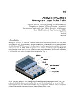
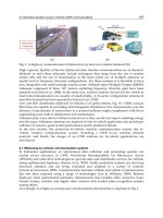
The overall experimental setup is shown in Figure 1.
The collected signals are processed with averaging method (Xu, 2001) to remove the signal

artifacts, which includes incident pulse, boundary reflection and multipath. The processing
is also known as calibration in the literature. Delay-and-sum beamforming (Xu, 2001)
algorithm is used to generate the image as in confocal imaging technique. Breast image is
formed by synthetically focusing the signals received from the antenna array to every point
within the region of interest.


Fig. 1. Overall experimental setup.
Ultra-Wideband Pulse-Based Microwave
Imaging for Breast Cancer Detection: Experimental Issues and Compensations

319
2. Pulse jitter artifact and compensation
As mentioned in the introduction, averaging method is applied to remove artifacts in the
received signals before delay-and-sum beamforming. An average of all received signals
from different antennas is calculated. The averaged signal is used as a template artifact and
is subtracted from individual received signals. Clean tumor responses can be obtained if the
system is free of noise. The processing is also known as calibration in the literature.
However, averaging method will not work well if the received signals are not aligned
perfectly and have unequal amplitudes. Pulse delay jitter is caused by the impulse generator
being unable to maintain a constant delay time between trigger signal and the output UWB
pulse. The maximum delay timing jitter measured with oscilloscope in the experiment is 31
ps. Pulse amplitude instability is caused by the impulse generator which is unable to
maintain constant amplitude of the output UWB pulse.
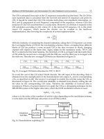
Figures 2 and 3 show that pulse instability causes phase shift of 31 ps or 20 sample points in
the signals. The resultant artifact would be large if the signals are not first compensated. For
phase jitter compensation, all received signals are aligned by finding the zero-crossing point
between maximum and minimum peaks and phase shifting the signals to the same zero-
crossing point. For amplitude instability, compensation is done by normalizing all the
signals peak-to-peak amplitude to one unit.

Fig. 2. Signals before and after pulse jitter compensation.

Novel Applications of the UWB Technologies

320

Fig. 3. Zoom in view of signals given in Figure 2.
To further minimize the phase error, the received signals are extrapolated to higher
sampling rates. Table 1 shows the phase error for received signals and resultant signal
artifact after pulse instability compensation at different extrapolated sampling rates.
Measured noise amplitude is obtained after applying averaging method to a set of data
collected from a tumor-free breast phantom. Simulated noise amplitude is calculated with
Matlab by subtracting two identical signals, one signal is phase shifted by one sample time
from another signal.
The noise amplitude shown in Table 1 is normalized to the incident pulse amplitude. The
measured noise amplitude does not further decrease with higher sampling rates greater
than 1 THz because the other contributors of noise such as environmental noise becomes
significant, whereas the simulated noise amplitude continues to decrease with higher
sampling rate as expected.

Sampling
Rate
Worst
Phase Error
Simulated
Noise Am
p

litude
Measured
Noise Am
p
litude
No compensatio
n
31.25 ps – 0.7866
40 GHz 25.00 ps 0.5437 0.5217
80 GHz 12.50 ps 0.2816 0.2781
160 GHz 6.25 ps 0.1684 0.1734
320 GHz 3.13 ps 0.0815 0.0942
640 GHz 1.56 ps 0.0533 0.0565
1 THz 1.00 ps 0.0344 0.0436
2 THz 0.50 ps 0.0173 0.0435
Table 1. Calculated and measured noise amplitude after pulse instability compensation at
different extrapolated sampling rates.
Ultra-Wideband Pulse-Based Microwave
Imaging for Breast Cancer Detection: Experimental Issues and Compensations

321
Figure 4 shows the effects of pulse instability compensation on images formed by delay-
and-sum beamforming. The tumor is located at 3 cm to the right from the center, or at
coordinate (130, 100). The pulse jitter artifact located at (150,130) is significantly suppressed.


Fig. 4. The effects of pulse instability compensation on breast phantom images. Left: without
compensation. Right: with compensation.
3. Real-time oscilloscope
This section discusses the dynamic range of Agilent DSO-081204B real-time oscilloscope

used in the experiment. The information of the dynamic range will determine whether the
pulse reflected from a tumor is too small to be detected. In this discussion, dynamic range is
defined as the ratio of the oscilloscope vertical-scale range and the amplitude of the smallest
possible digitized pulse.
Agilent DSO-081204B real time oscilloscope has analog-to-digital converters (ADC) with 8-
bit resolution. After averaging and interpolation, the oscilloscope is able to increase the
vertical resolution and store the data in 16-bit resolution. Due to quantization of the signal,
at least 4-bit resolution is needed to construct the pulse shape of tumor response as shown in
Figure 5. So the remaining 12-bit range is the maximum dynamic range of the oscilloscope.


Fig. 5. Ideal tumor response constructed with 2-bit, 4-bit, and 6-bit vertical resolutions
showing that the minimum required resolution is 4 bits.
An experiment is conducted to determine the dynamic range of the oscilloscope by
investigating its ability to construct a pulse. Due to the presence of noise, a pulse cannot be
observed from a single signal. Instead, 360 sets of signals are collected and an averaged

Novel Applications of the UWB Technologies

322
signal is obtained. The random noise will be averaged out, and the pulse can be observed if
it is within the dynamic range.
The incident pulse is set very small so that its amplitude is equal to the expected smallest
peak for different possible dynamic range as shown in the Table 2. The recorded signals are
averaged to determine at which dynamic range the pulse can still be constructed.

12
8
0.002
2

Fullrange voltage
V
Ex
p
ected
p
eak V
Dynamicrange
bits

(1)
From the experiment, , the pulse cannot be seen from the averaged signals if its amplitude is
set to 2 mV, while the maximum noise amplitude is 5.9 mV. Whereas for a pulse amplitude
of 4mV, the pulse is merely noticeable at sample time 1600 as shown in Figure 6. From this
experiment which considers the system noise, the dynamic range is estimated to be 11-bits,
which has 2048 values available for the whole range. Thus, the maximum detectable ratio
between incident pulse and tumor response is 2048.

Dynamic Range
2^
Smallest peak
can be detected
Recorded
peak
8bits 31mV 33.2mV
9bits 16mV 14.9mV
10bits 8mV 7.8mV
11bits 4mV 6.1mV
12bits 2mV 5.9mV
Table 2. Expected and recorded peak of incident pulse for different dynamic range.

Fig. 6. Constructed pulse to test dynamic range of 2
11
bits. The pulse is just noticeable at
sample 1600. Upper trace shows the 360 signals and lower trace shows the averaged signal.
Ultra-Wideband Pulse-Based Microwave
Imaging for Breast Cancer Detection: Experimental Issues and Compensations

323
4. Ring artifact
If the experiments use a breast phantom with higher permittivity, ring artifacts will appear
as shown in Figure 7. The phantom is fabricated using tissue mimicking phantom material
(Lazebnik, 2005) with 80% oil, contained in a polypropylene cylindrical container (diameter
16cm, height 12cm). The material is able to closely simulate the dielectric properties of
human tissues.
Tumor simulant is an 8 mm cube made of phantom material with 10% oil buried at 25 mm
right from center of the phantom. The measured dielectric constant at 5 GHz for phantom
medium is 9 whereas for tumor is 50 which is representative of normal and malignant
human breast tissues. Ring artifacts have not been reported previously by other researchers
because their breast phantoms use only lower dielectric constant materials.


Fig. 7a. Images of breast phantom with 1 mm off-center positioning error (left) and breast
phantom less than 0.5 mm off-center error (right).


Fig. 7b. Same Images from Figure 7a with correlation applied.
Ring artifact arises from positioning error (off-center) of the breast phantom. Ideally,
averaging method works perfectly with round phantom. Ring artifact appears when the

phantom is not positioned perfectly on the rotary axis of the experimental stage. This causes
small displacement error of the phantom boundary relative to the antennas.
Ring artifact is caused by the coherent adding of the residue boundary reflections after
delay-and-sum beamforming. The ring-to-ring distance is proportional to the wavelength of

Novel Applications of the UWB Technologies

324
the incident signal. Ring artifact also indicates the direction of phantom off-center
displacement. For instance, when the phantom is displaced to right side, the ring artifact
will appear on right indicating positive x-axis off-center displacement and left indicating
negative x-axis off-center displacement.
In experiments with oil medium which has lower dielectric constant, ring artifact is not
noticeable because the tumor response is large enough to dominate the ring artifacts in the
image. The correlation method is not able to improve the image quality when ring artifacts
arise as illustrated in Figure 7b. This is due to the high similarity between tumor response
and the residue incident pulse ringing.
Adjusting the phantom to the best position using visual inspection will result in a
positioning error of 1 mm to 3 mm. Better placement can be achieved by placing a reference
object on the antenna to measure the antenna to phantom boundary distance and adjusting
the phantom position until the error is smaller than 0.5 mm. The resulting ring artifact is
reduced significantly.
4.1 Experiment on ring artifact
An experiment is conducted to test the amplitude of the ring artifact for different
displacement errors of a breast phantom without tumor. The phantom is adjusted to the best
position with error less than 0.5 mm. Measurements are taken for the phantom at best
position, then with off-center displacements of 1 mm, 2 mm, and 3 mm from the best
position. The resultant signal artifact shown in Table 3 is computed after applying averaging
method. When the breast phantom is perfectly positioned, the signal artifact should be zero.

Position error
Artifact RMS
Amplitude (x10
-3
)
Artifact P-P
Amplitude (x10
-3
)
<0.5 mm 1.0 2.3
1 mm 3.3 5.7
2 mm 5.5 9.9
3 mm 8.7 15.0
Table 3. Averaged RMS and peak-to-peak amplitude of signal artifact after averaging
method for different off-center positioning errors.
5. Loss compensation
This section discusses the power loss during propagation of UWB pulse in breast medium,
and the loss models used for compensation. Loss can be contributed by the radial spreading
of UWB pulse originating from the antenna as well as attenuation caused by the breast
medium. Loss compensation is a signal processing step to equalize all the received signals
originating from different locations such that the whole scanning region has unity gain.
5.1 Radial spreading loss
Most studies approximate the propagating signal as a uniform cylindrical wave and thus the
radial spreading loss equal to 1/r, where r is distance from antenna to the particular
scanning point. Considering both transmit and receive paths make the loss proportional to
distance square. Compensation is done by multiplying the signals by r
2
. Figure 8 shows the
decrease of reflected signal amplitude from a tumor considering only radial spreading loss.
The tumor is located nearest to the antenna at 0 degree and furthest at 180 degrees.

Ultra-Wideband Pulse-Based Microwave
Imaging for Breast Cancer Detection: Experimental Issues and Compensations

325

Fig. 8. Simulated received pulse amplitude considering only radial spreading loss.
5.2 Effects of loss compensation
To see the effects of loss compensation, compensation is applied on experiment data to
compare the results obtained without compensation applied.
Imaging results in Figure 9 show that loss compensation tends to amplify noise near the
phantom boundary. The compensation applied here is only considering radial spreading
loss. Worse results will be expected if other loss factors are incorporated, since the signals
are multiplied by larger factors.
Radial spreading compensation is a commonly used signal processing step in breast cancer
detection algorithms in numerical noise-free modeling. In view of the deteriorating effects of
radial spreading compensation on image quality, it is recommended not to apply the
compensation.





Fig. 9. Image with radial spreading compensation (left) and without radial spreading
compensation (right).

Novel Applications of the UWB Technologies

326
6. Filtering and correlation
This section describes two signal processing methods applied to improve the signal-to-noise

ratio (SNR) of the breast phantom images.
6.1 Filtering
The ultra-wideband (UWB) antenna used in the experiments has a bandwidth of 1.8 to 6.3
GHz. Two significant narrowband interferences for the experiments conducted are cell
phone noise at 1.8 GHz and wireless local area network (LAN) noise at 2.4 GHz. Thus,
digital notch filters at 1.8 GHz and 2.4 GHz are applied to reduce the interferences. The
signals and power spectra before and after filtering applied are given in Figure 10. The
image quality has been improved with filtering as shown in Figure 11.

















Fig. 10a. Signals (upper trace) and power spectra (lower trace) before filtering.
Ultra-Wideband Pulse-Based Microwave
Imaging for Breast Cancer Detection: Experimental Issues and Compensations

327

Fig. 10b. Signals (upper trace) and power spectra (lower trace) after filtering.







Fig. 11. Images formed without filtering (left) and with filtering applied (right). The tumor is
located at 3 cm to the right of the center.

Novel Applications of the UWB Technologies

328
6.2 Correlation
A tumor response template is created in Matlab as shown in Figure 12. Correlation is
applied by multiplying the tumor response with the filtered signals after the delay-and-sum
operation at each pixel. Then the signals are windowed and summed to give a value for
every pixel in the breast phantom image given in Figure 13. The image quality has been
enhanced with correlation.


Fig. 12. Tumor response template.

Fig. 13. Comparison for filtered images without correlation (left) and with correlation (right).
The discussion above focuses on only a single experiment data. The result may not be
representative as the occurrences of artifacts in images are random due to coherence
alignment of noise at certain points. Thus large scale experiments are performed to study
the effect of applying filtering and correlation on breast phantom images. Ten experiments
are conducted with the same experimental setup and breast phantom. Tumor simulant is at
position (130, 100) for all experiments. Experiments are repeated with different antennas
array of 6, 12, 24, and 36 elements in one phantom rotation. Forty sets of data are collected
and processed. A total of 80 images are formed for SNR analysis. Figure 14 show 20 images
from experiments conducted with 24 antennas array.
Ultra-Wideband Pulse-Based Microwave
Imaging for Breast Cancer Detection: Experimental Issues and Compensations

329
SNR is calculated from the ratio of the pixel value at tumor location (130, 100) over the
highest value of noisy pixels 6 mm radius outside the tumor location. Since the SNR value
from individual experiment is highly variable, due to random occurrences of artifacts, an
averaged SNR value is calculated using ten SNR values from ten experiments.
Detectability is the ability to observe the tumor in the images although the tumor may not
appear as the strongest pixel. Detectability is defined as one when the tumor pixel value is
above half of the maximum scale and above twice of the adjacent region pixel values,
otherwise zero is given for that image. Table 4 shows that detectability is at least 80% when
SNR is positive.
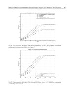
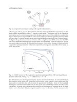
Figure 15 show the SNR versus number of antennas per phantom. There is a significant
improvement on SNR with correlation applied. Increasing the number of antennas improves
the SNR but cost and complexity of implementation increases. To archive positive SNR, the
minimum number of antennas needed without correlation is 12 compared to 10 for
correlation.

Fig. 14a. Ten filtered images without correlation applied.




Fig. 14b. Ten filtered images with correlation applied.

Novel Applications of the UWB Technologies

330
SNR Array of 6 Array of 12 Array of 24 Array of 36
Delay & Sum -8.7 dB -3.6 dB -0.3 dB 4.3 dB
Filtering -6.3 dB 0.5 dB 6.1 dB 8.2 dB
Correlation -5.7 dB 3.5 dB 11 dB 13 dB
Detectability Array of 6 Array of 12 Array of 24 Array of 36
Delay & Sum 0/10 5/10 8/10 10/10
Filtering 1/10 8/10 10/10 10/10
Correlation 2/10 10/10 10/10 10/10
Table 4. SNR and detectability for different antennas arrays.


S NR v s N um be r o f A nt e nna s
-10
-5
0
5

10
15
010203040
Nu m be r o f A n te n nas
SNR (dB
)
Delay & Sum
Fi lt ering
Correl ati on

Fig. 15. SNR versus number of antennas.
To study the robustness of the correlation method, the tumor stimulant is positioned at
different distances, 1 cm to 6 cm, from the center of the breast phantom with the experimental
results given in Figure 16. Images in Figure 16 show that correlation improves the image
quality.
Ultra-Wideband Pulse-Based Microwave
Imaging for Breast Cancer Detection: Experimental Issues and Compensations

331

Fig. 16. Images formed without correlation (top) and with correlation (bottom), with tumor
located 1 cm to 6 cm from center.
7. Signal and image SNR
This section discusses the effects of improving the image SNR by increasing the averaging
number and antenna number. The tradeoff of increasing these two factors is the increase of
acquisition time.
In most other studies, an array of only a few antennas are considered as more antennas do
not improve the image resolution but at higher simulation time. However, the advantage of
more antennas is noise reduction. Better image SNR can be obtained by increasing the
averaging number and antenna number.

Some terms used in the discussion are defined as follows:

Averaging number is the number of waveforms acquired by the oscilloscope to
produce an averaged waveform for each acquisition at one antenna position.

Antenna number is the number of antennas in the synthetic array around the
circumference of the phantom. It is also the number of steps for a complete
phantom rotation relative to a stationary antenna.

Signal SNR is the ratio of the root mean square (RMS) value of averaged tumor
response to the RMS value of the averaged noise.

Image SNR is the ratio of the tumor pixel intensity to the highest-value artifact
pixel intensity. The definition differs from SCR which is Signal-to-Clutter Ratio,
since there is no clutter considered in this discussion. Artifact pixels are caused by
coherent summation of noise and occur randomly whereas clutters remain at their
positions and averaging is unable to remove them.
7.1 SNR improvement with larger averaging and antenna number
Signal SNR can be improved by using larger averaging number, whereas image SNR can be
improved by using larger antenna number.
To measure the noise level, antenna is placed stationary without the presence of breast
phantom or any moving object. Incident pulse amplitude is set to different attenuation
setting from 0 dB (8 V) to 24 dB (0.5 V). A total of 360 measurements with only incident
pulse are taken as in breast scanning. Noise is calculated by subtracting the individual
measurement with the average measurements. The RMS and peak-to-peak noise is shown in

Novel Applications of the UWB Technologies

332
Table 5 and Figure 17, which is the average of 360 noise amplitudes relative to the incident

pulse amplitude.

Averaging
1 4 16 64 256 1024 4096
RMS noise
4.8 mV 1.7mV 0.83 mV 0.45 mV 0.24 mV 0.15 mV 0.10 mV
Table 5. RMS amplitude of noise for different averaging number with maximum pulse
amplitude of 8V (attenuation setting 0 dB).


0.1
1
10
100
1 10 100 1000 10000
RMS Noise (mV)
Averaging No.
RMS noise vs Averaging No.
0dB
6dB
12dB
18dB
24dB

Fig. 17. RMS noise versus averaging number for different pulse attenuation settings.
Matlab simulations are conducted to determine the image SNR. Ten sets of UWB noise are
created by applying a bandpass filter to white noise with all the resultant noise RMS
amplitudes set to 0.5 mV. The noise is scaled to the noise RMS amplitude of different
averaging numbers as shown in Table 5 and added to the ideal tumor response as shown in
Figure 12. The tumor response has peak-to-peak amplitude of 1 mV and RMS of 0.2567 mV.

The signals are delayed as though they are received from the 360 antennas spaced regularly
around the breast phantom. The same delay factors are used in creating the signals and in
subsequent beamforming. Thus there is no error caused by delay estimation. A total of 120
sets of data are created for confocal imaging for each antenna number of 12, 24, 45, 90, 180,
and 360.
Since the image SNR is random due to random occurrences of artifacts, ten SNR values are
obtained and averaged based on simulation with ten sets of data for each averaging number
and antenna number. A total of 720 images are produced from the simulations. The results
are summarized in Table 6 and Figure 18.
Ultra-Wideband Pulse-Based Microwave
Imaging for Breast Cancer Detection: Experimental Issues and Compensations

333



Antenna
No.
12 24 45 90 180 360
Averaging
No.
Signal
SNR
Image SNR
2 -18.66
-2.8 -2.8 -2.2 -2.4 -2.0 -1.3
4 -15.89
-2.8 -2.8 -2.1 -2.1 -1.4 0.0
8 -13.4
-2.7 -2.7 -1.9 -1.7 -0.2 1.7

16 -10.09
-2.6 -2.2 -1.3 -0.2 1.9 4.0
32 -7.08
-2.3 -1.3 -0.2 1.9 4.0 5.8
64 -4.68
-1.9 -0.2 1.3 3.8 5.5 6.8
128 -2.69
-1.2 1.1 2.6 5.1 6.5 7.5
256 -0.11
0.3 2.8 4.4 6.4 7.4 8.1
512 2.17
1.9 4.3 5.7 7.2 8.0 8.6
1024 3.58
2.9 5.2 6.4 7.7 8.3 8.8
2048 6.6
4.8 6.5 7.5 8.4 8.8 9.1
4096 8.19
5.6 7.1 8.0 8.7 9.0 9.2

Table 6. Image SNR for different averaging number and antenna number. Signal SNR is
calculated with tumor response RMS of 0.2567 mV.
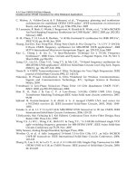
Images from the simulations are shown in Figures 19, 20, and 21 for different sets of noise,
noise amplitudes, and antenna numbers. As observed from Figure 18, the cost to increase
the image SNR is getting higher when the signal SNR is positive. When the signal SNR is
negative, the cost to increase the image SNR is lower. In other word, it is worth using array
of more antennas when the tumor response received is weaker than the noise.
In this simulation, the amplitude of the tumor response is fixed at 1 mV, with RMS value of
0.2567 mV. The tumor response is 1000 times smaller than the 1V incident pulse. In this case,
we could use antenna number of 12 and averaging number of 1024 to produce reasonably
good results.

Novel Applications of the UWB Technologies

334







Fig. 18. Image SNR versus Signal SNR for different antenna numbers.








Fig. 19. Images obtained with ten sets of noise processed with antenna number of 360 and
RMS noise level of 2.2 mV.
Ultra-Wideband Pulse-Based Microwave
Imaging for Breast Cancer Detection: Experimental Issues and Compensations

335



Fig. 20. Images obtained with the same set of noise processed with antenna number of 360

and RMS noise level from 2.2 mV (top left) to 0.10 mV (bottom right).


Fig. 21. Images obtained with the same set of noise processed with antenna number of 12
(top left), 24, 45, 90, 180, 360 (bottom right) and RMS noise level of 0.45 mV.
8. Conclusion
In this chapter, experimental study of UWB breast cancer detection in time domain and
several important experimental issues are discussed. These include pulse jitter artifact,
dynamic range of oscilloscope, ring artifact caused by positioning error, noise amplification
caused by radial spreading loss compensation, noise reduction after applying filtering and
correlation, as well as the improvement on signal SNR and image SNR by using larger
averaging and antenna number. The identified issues and compensation methods will
facilitate the future experiments in UWB breast cancer detection with more realistic breast
phantoms.

Novel Applications of the UWB Technologies

336
9. References
Bond E. J., Li X., Hagness S. C., & Van Veen B. D. (2003). Microwave Imaging via Space-
Time Beamforming for Early Detection of Breast Cancer,
IEEE Transactions on
Antennas and Propagation
, vol. 51, no. 8, pp. 1690-1705, ISSN 0018-926X
Chua L. W. (2005). A new UWB antenna with excellent time domain characteristics,
Proceedings of The European Conference on Wireless Technology, ISBN: 2-9600551-1-X,
Paris, October 2005.
Lazebnik M., Madsen E. L., Frank G. R., and Hagness S. C. (2005). Tissue-mimicking
phantom materials for narrowband and ultrawideband microwave applications,
Physics in Medicine and Biology, vol. 50, no. 18, pp. 4245-4258, ISSN 0031-9155

Sill J. M. & Fear E. C. (2005). Tissue sensing adaptive radar for breast cancer detection -
experimental investigation of simple tumor models,
IEEE Transactions on Microwave
Theory and Techniques
, vol. 53, no. 11, pp. 3312-3319, ISSN 0018-9480
Xu Li & Hagness S. C. (2001). A Confocal Microwave Imaging Algorithm for Breast Cancer
Detection,
IEEE Microwave and Wireless Components Letters, vol. 11, no. 3, pp. 130-
132, ISSN 1531-1309
Xu Li, Davis S. K., Hagness S. C., van der Weide D. W., & Van Veen B. D. (2004). Microwave
Imaging via Space-Time Beamforming: Experimental Investigation of Tumor
Detection in Multi-Layer Breast Phantoms,
IEEE Transactions on Microwave Theory
and Techniques
, vol. 52, no. 8, pp. 1856-1865, ISSN 0018-9480
0
Frequency Domain Skin Artifact Removal Method
for Ultra-Wideband Breast Cancer Detection
Arash Maskooki, Cheong Boon Soh, Erry Gunawan and Kay Soon Low
Nanyang Technological University
Singapore
1. Introduction
According to the Center for Disease Control and Prevention (CDC) (Center for Disease Control
and Prevention (CDC), 2007) and American Cancer Society (ACS) (American Cancer Society
(ACS), 2007), breast cancer is the most prevalent type of cancer among women only after
skin cancer and the number two cause of cancer death in women. Among every 8 women
in U.S. one has breast cancer. In addition, about 2.5 million survivors of breast cancer are
living in the United States and it is estimated that 40,170 lives perished due to this mortal
disease in 2009. Many risk factors have been associated with breast cancer including, but
not limited to, gender, age, family history, race and lifestyle (American Cancer Society (ACS),

2007). Some of these risk factors could not be controlled such as age or family history. In
contrast, factors such as life style could be changed to prevent or reduce the chance of breast
cancer. Various techniques are practiced today for treating breast cancer. Nevertheless, in all
treatment methods early detection is a crucial factor. Detecting breast cancer in early stages
can lead to more efficient treatment and comfort for the patient. Hence, an accurate diagnosis
modality for breast cancer detection can save many lives annually.
Currently, X-Ray mammography is the gold standard method in detecting breast cancer and
is used widely due to relatively easy access to the equipment. In this method, a low dose
of X-Ray is used to obtain a mapping of the distribution of the tissue density inside the
compressed breast. Mammography can be used for both screening and diagnosis of breast
cancer. In screening mammography, X-Ray imaging of the breast is used in women with no
signs of the breast cancer for the purpose of investigation of the breast tissue changes and
examining the lesions inside the breast. As a diagnostic tool, X-Ray mammography could
be used to assess the malignancy of the lesions that has already been found in the breast. It
has been shown that mammography can reduce the mortality rate due to breast cancer (J.
Elwood and B. Cox and A. Richardson, 1993) because detecting breast cancer in the early
stages can lead to a more efficient treatment. Although X-Ray mammography has benefits
such as ease of use, availability and being reasonably accurate, it is not a perfect method for
screening and diagnosing breast cancer. A major drawback of X-Ray mammography is the
danger of exposing the patient to a low dose of ionizing radiation which can increase the risk
of cancer. This makes X-ray mammography a less suitable tool for screening and more suitable
for diagnosis. In addition, to avoid a blurred image and preserve the uniformity of the tissue,
the breast is compressed before X-Ray imaging which can be uncomfortable for the patients
(Fear et al., 2002).
16
2 Will-be-set-by-IN-TECH
Another modality based on Ultra-Wide Band (UWB) pulse confocal imaging radar for
screening and possibly diagnosis of breast cancer has been suggested and investigated in
recent years (Li & Hagness, 2001). UWB imaging of the breast employs malignant tissue’s
significant dielectric contrast to detect the location of the tumor relative to an antenna array. To

obtain a 2-D or 3-D (depending on the application) map of dielectric contrast inside the breast
medium, an array of antenna around the breast transmit a UWB pulse sequentially and record
the backscattered signal. In the next step, the backscattered signals are synthetically focused at
a synthetic focal point. To focus the beam at the synthetic focal point, the travel time between
the antenna and the synthetic focal point is calculated and the energy received from that point
in all channels in the antenna array are added together. Existence of a strong scattering point
(high contrast in dielectric value) at the synthetic focal point results in a coherent summation
of pulse energy and hence a high total energy value assigned to that point. On the other
hand, if no scattering point is present at the synthetic focal point, energy values will add
incoherently and the total energy value assigned to that location won’t be so high. To produce
a 2D or 3D image of the breast region, the synthetic focal point is scanned through all the
breast region and the summation of the acquired energy values are mapped as the pixel value
at that location.
In contrast to the X-ray mammography, UWB confocal imaging does not expose the patient to
any ionizing radiation. This means that it can be used frequently as an screening tool specially
for younger women. In addition, the uncomfortable breast compression is eliminated is this
modality.
Although it has been shown that the cancerous tumors can be located by UWB breast imaging,
there are still issues that must be addressed. One of these issues is the problem of the surface
skin backscatter. Human breast skin has a high dielectric contrast with both air and skin tissue.
This will produce a strong backscatter from the skin surface in the received signal. Although
skin backscatter has its major components in the early time of the received signal, it continues
to affect parts of the late time response. The problem is that the late time effects of the skin
backscatter are still strong enough to mask the weak tumor reflection completely. Hence, the
skin effects should be removed from the response prior to the imaging process. A simple
method to remove the skin artifact is to mask out the early time part of the signal. However,
as mentioned before, skin artifact continues its effect to the late time response and masking out
the early time part of the signal would not remove the late time effects. Another problem of
the simple masking method is that prior to the imaging process the location of the tumor is not
known. Hence, masking the early time part of the signal might remove the tumor reflection.

A more practical method has been suggested by researchers based on averaging. In averaging
method, the backscattered signal is averaged over all signals from different antennas in the
array. The average is then subtracted from the individual signals. The idea is that the skin
reflection would appear in the average because it is similar in all channels and will add
coherently, but the tumor response has different locations in different channels and would
not add up coherently and hence would not appear in the average. Although averaging can
significantly suppress the early time portion of the skin reflection, it is not able to remove
the late time parts of the artifact. In addition, averaging removes parts of the reflection from
the tumor especially in cases where the tumor is equidistant from different antennas. As an
improvement over averaging, an averaging based filtering process is proposed in literature
to remove the skin artifact. Although filtering greatly improves the skin backscatter removal,
it still deteriorates the tumor response. Furthermore, the same as averaging method, it will
338
Novel Applications of the UWB Technologies
Frequency Domain Skin Artifact Removal Method for Ultra-Wideband Breast Cancer Detection 3
remove the tumor reflection together with the skin artifact when the tumor is equidistant to
several antennas in the array.
This chapter introduces a frequency domain approach to the skin artifact removal problem
in UWB breast cancer detection. In this approach, the received signal is first converted into
the frequency domain. Then, the skin related information is identified and removed from the
frequency domain response. The signal is then converted back to the time domain and used
for the imaging process. This approach does not affect the tumor response as it processes
each signal individually and does not incorporate any subtraction or addition to the signals.
Besides, the skin reflection is eliminated from both early time and late time responses. In
addition, it is shown that the frequency domain approach can preserve the tumor response
when the tumor is located equidistant to all antennas in the array, such as central axis of
the array. Using computer simulations, the frequency domain approach is compared with the
existing averaging based methods in different scenarios and is shown to be able to outperform
the current existing methods.
This chapter is organized as follows. The next section provides a brief overview of the confocal

imaging method in UWB breast cancer detection. In Section 3, the skin artifact problem and
existing methods to overcome this problem are described. Section 4 introduces the frequency
domain approach to remove the skin artifact. In Section 5, performance of the frequency
domain approach is compared with the existing methods through computer simulations in
different cases and each case is discussed in detail. Finally, Section 6 will conclude this chapter.
2. Confocal Microwave Imaging (CMI) in UWB breast imaging
To obtain the tumor signature, breast is illuminated by a UWB microwave pulse from a
number of antennas arranged in a planar configuration over the breast or in a circular
configuration around the breast (Fear et al., 2002). Due to the contrast between dielectric
properties of the tumor and the normal breast tissue, malignant tumors have a significant
scattering cross section compared to the normal tissue and benign tumor types (Hagness et al.,
1998). To obtain a high resolution in the imaging process, the pulse bandwidth has to be as
high as possible. However, frequencies higher than 10 GHz will face a dramatic attenuation
inside the human body and the breast medium. Hence, the upper limit for frequency content
of the signal is about 10 GHz. This limit ensures enough penetration for human breast imaging
(Fear & Stuchly, 2000).
To obtain enough penetration for the UWB imaging of the breast, the antenna is excited by a
differentiated Gaussian pulse (Fear et al., 2002):
V
(t)=(t −t
0
)e
−(
t−t
0
τ
)
2
(1)
where t

0
= 4τ and τ = 0.0625ns. The resulting signal has temporal duration (full-width
half-maximum) of 0.17 ns and approximately 6 GHz bandwidth with maximum power near to
4GHz. Figure 1 shows the temporal pulse shape and its frequency spectrum (Fear et al., 2002).
The heterogeneous nature of the breast medium produces clutter in the UWB signature of the
tumor which makes detecting the tumor difficult or in some cases impossible. To overcome
this problem, a modified version of UWB Ground Penetrating Radar (GPR) is suggested for
breast medium to amplify the tumor signature and eliminate the clutter (Hagness et al., 1998).
In this method, clutter suppression is carried out by coherent addition of the tumor responses
from all channels. To spatially focus the signal at the candidate location, the backscattered
339
Frequency Domain Skin Artifact Removal Method for Ultra-Wideband Breast Cancer Detection
4 Will-be-set-by-IN-TECH
(a) Differentiated Gaussian Pulse (b) Frequency Spectrum of Differentiated Gaussian
Pulse
Fig. 1. Pulse Waveform
Fig. 2. A time window is applied on different channel responses in Confocal Imaging Process
signal is time shifted and summed based on the pulse travel time to the synthetic focal point.
The energy value of the windowed portion of the signals from all the channels are calculated
and summed up to form a pixel value for the image of the breast. The synthetic focal point
is then scanned through the entire breast medium by appropriately changing the time shifts
and windowing to achieve a 2D or 3D image of the breast. As mentioned before, existence
of a strong scatterer at the synthetic focal point would produce a replica of the pulse at the
corresponding time instance in the backscattered signal in all channels. Hence, summation
of this portion of the response from all channels yields a high energy value which points to
the existence of a scatterer. However, if only clutter and noise are the dominant components
at the focal point, the energy levels do not add coherently and the clutter will be suppressed
(Fear & Stuchly, 2000). Figure 2 depicts the windowing and summation process. The window
length is chosen equal to the temporal duration of the original pulse to include the whole
backscattered energy.

340
Novel Applications of the UWB Technologies
Frequency Domain Skin Artifact Removal Method for Ultra-Wideband Breast Cancer Detection 5
3. Skin backscatter removal
The signal received by the antenna contains contributions from lesions in the breast, clutter
due to heterogeneity of the tissue and skin backscatter. The skin backscatter artifact is in
the orders of magnitude larger than the other parts of the signal and can swamp the tumor
response. Thus, to detect the tumor, skin response should be removed from the signal. This
section describes and reviews the existing skin artifact removal algorithms.
3.1 Time window
The simplest way to get rid of the skin artifact is to mask out the early time part of the
response. This method could be considered as multiplying a time window which is a step
function of zero amplitude when the skin response exists and amplitude one in the rest of
the time interval (Zhi & Chin, 2006). However, this method could not be used in practice.
The problem is that there is no clear border between early time and late time parts of the
backscattered signal. In addition, skin reflection can be present in the late time response and
mask the tumor backscatter. Hence masking the early time part of the signal may remove
the tumor response as well. This is because the location of the tumor reflection is not a priori
information.
3.2 Averaging
A more practical method to remove the skin reflection from the backscattered signal is to use
the average of all channels to reconstruct and remove the skin reflection (Li & Hagness, 2001).
In this method, the average of the backscattered responses from several antenna elements
is subtracted from the response of each element. The idea in averaging method is that the
skin response is similar in different channels. This is because the skin structure is assumed
symmetric in the view of all elements of the antenna array. To compensate for the variations
in each element’s distance from skin surface, all responses are aligned to the local maximum
of the early time response (which corresponds to the skin backscatter). When the signals
in different channels are averaged, the similar parts such as skin backscatter will add up
coherently and hence appear in the averaged signal. However, other reflections such as tumor

and clutter backscatters differ in amplitude and location from channel to channel. The tumor
reflection is at different time instants in different channels. This is because of the difference
in the relative distance of the tumor to each antenna element. Hence the tumor signature
will add incoherently in the averaging process and is suppressed in the average signal. Thus,
removing the average from the signal removes mostly the skin artifact.
Averaging best works when the skin reflection is similar in all channels. In such case, it can
totally remove skin artifact from the data. Nevertheless, skin structure is not the same all
over the breast and this affects the similarity of the skin reflections at different receivers. One
of the factors that changes the skin response in different locations is the variation in skin
thickness in different parts of the breast (Ulger et al., 2003). Another contributing factor is the
heterogeneity of the breast tissue under the skin surface which can cause variations in the skin
backscatter.
As mentioned above, skin response does vary from channel to channel and this variation
affects the ability of the averaging in removing the skin artifact thoroughly. Another inherent
problem of the averaging method is the distortion to the possible tumor reflection. This is
because during the averaging process the tumor and clutter responses from all channels are
added and averaged incoherently. This average is then subtracted from each channel and
341
Frequency Domain Skin Artifact Removal Method for Ultra-Wideband Breast Cancer Detection