Standard Methods for Examination of Water & Wastewater_2 ppt
Bạn đang xem bản rút gọn của tài liệu. Xem và tải ngay bản đầy đủ của tài liệu tại đây (893.42 KB, 30 trang )
Part II
Unit Operations of Water
and Wastewater Treatment
Part II covers the unit operations of flow measurements and flow and quality equal-
izations; pumping; screening, sedimentation, and flotation; mixing and flocculation;
filtration; aeration and stripping; and membrane processes and carbon adsorption.
These unit operations are an integral part in the physical treatment of water and
wastewater.
TX249_frame_C03.fm Page 179 Friday, June 14, 2002 4:22 PM
© 2003 by A. P. Sincero and G. A. Sincero
Flow Measurements
and Flow and Quality
Equalizations
This chapter discusses the unit operations of flow measurements and flow and quality
equalizations. Flow meters discussed include rectangular weirs, triangular weirs,
trapezoidal weirs, venturi meters, and one of the critical-flow flumes, the Parshall
flume. Miscellaneous flow meters including the magnetic flow meter, turbine flow meter,
nutating disk meter, and the rotameter are also discussed. These meters are classified
as miscellaneous, because they will not be treated analytically but simply described.
In addition, liquid level recorders are also briefly discussed.
3.1 FLOW METERS
Flow meters
are devices that are used to measure the rate of flow of fluids. In
wastewater treatment, the choice of flow meters is especially critical because of the
solids that are transported by the wastewater flow. In all cases, the possibility of
solids being lodged onto the metering device should be investigated. If the flow has
enough energy to be self-cleaning or if solids have been removed from the waste-
water, weirs may be employed. Venturi meters and critical-flow flumes are well
suited for measurement of flows that contain floating solids in them. All these flow-
measuring devices are suitable for measuring flows of water.
Flow meters fall into the broad category of meters for open-channel flow mea-
surements and meters for closed-channel flow measurements. Venturi meters are
closed-channel flow measuring devices, whereas weirs and critical-flow flumes are
open-channel flow measuring devices.
3.1.1 R
ECTANGULAR
W
EIRS
A
weir
is an obstruction that is used to back up a flowing stream of liquid. It may
be of a thick structure or of a thin structure such as a plate. A
rectangular weir
is
a thin plate where the plate is being cut such that a rectangular opening is formed
in which the flow in the channel that is being measured passes through. The rectangular
opening is composed of two vertical sides, one bottom called the
crest
, and no top
side. There are two types of rectangular weirs: the suppressed and the fully contracted
weir. Figure 3.1 shows a fully contracted weir. As indicated, a
fully contracted
rectangular weir
is a rectangular weir where the flow in the channel being measured
contracts as it passes through the rectangular opening. On the other hand, a
sup-
pressed rectangular weir
is a rectangular weir where the contraction is absent, that
3
TX249_frame_C03.fm Page 181 Friday, June 14, 2002 4:22 PM
© 2003 by A. P. Sincero and G. A. Sincero
182
Physical–Chemical Treatment of Water and Wastewater
is, the contraction is suppressed. This happens when the weir is extended fully across
the width of the channel, making the vertical sides of the channel as the two vertical
sides of the rectangular weir. To ensure an accurate measurement of flow, the crest
and the vertical sides (in the case of the fully contracted weir) should be beveled
into a sharp edge (see Figures 3.2 and 3.3).
To derive the equation that is used to calculate the flow in rectangular weirs,
refer to Figure 3.2. As shown, the weir height is
P
. The vertical distance from the
tip of the crest to the surface well upstream of the weir at point 1 is designated as
H
.
H
is called the
head
over the weir.
FIGURE 3.1
Rectangular weir measuring assembly.
FIGURE 3.2
Schematic for derivation of weir formulas.
Recording drum
Indicator
scale
Float
Connecting pipe
Float well Rectangular weir
Weir
Fully
contracted
flow
Crest
Top view
Weir
Contraction
L
1
J
1
J
2
J
c
P
Nappe
2
H
Weir
Rectangular weir
Beveled edge
of crest of weir
TX249_frame_C03.fm Page 182 Friday, June 14, 2002 4:22 PM
© 2003 by A. P. Sincero and G. A. Sincero
Flow Measurements and Flow and Quality Equalizations
183
From fluid mechanics, any open channel flow value possesses one and only one
critical depth. Since there is a one-to-one correspondence between this depth and
flow, any structure that can produce a critical flow condition can be used to measure
the rate of flow passing through the structure. This is the principle in using the
rectangular weir as a flow measuring device. Referring to Figure 3.2, for this structure
to be useful as a measuring device, a depth must be made critical somewhere. From
experiment, this depth occurs just in the vicinity of the weir. This is designated as
y
c
at point 2. A one-to-one relationship exists between flow and depth, so this section
is called a
control section
. In addition, to ensure the formation of the critical depth,
the underside of the nappe as shown should be well ventilated; otherwise, the weir
becomes submerged and the result will be inaccurate.
Between any points 1 and 2 of any flowing fluid in an open channel, the energy
equation reads
(3.1)
where
V
,
P
,
y
,
z
, and
h
l
refer to the average velocity at section containing the point,
pressure at point, height of point above bottom of channel, height of bottom of
channel from a chosen datum, and head loss between points 1 and 2, respectively.
The subscripts 1 and 2 refer to points 1 and 2.
g
is the gravitational constant and
γ
is the specific weight of water. Referring to Figure 3.2, the two values of
z
are zero.
V
1
called the
approach velocity
is negligible compared to
V
2
, the average velocity
at section at point 2. The two
P
s are all at atmospheric and will cancel out. The
friction loss
h
l
may be neglected for the moment.
y
1
is equal to
H
+
P
and
y
2
is very
closely equal to
y
c
+
P
. Applying all this information to Equation (3.1), and changing
V
2
to
V
c
, produces
(3.2)
FIGURE 3.3
Various types of weirs.
Channel walls
Thin plate Thin plate Thin plate
Suppressed
rectangular
weir
Triangular
weir
Trapezoidal
weir
L
a
b
c
e
d
e
r
V
1
2
2g
P
1
γ
y
1
z
1
h
l
–+++
V
2
2
2g
P
2
γ
y
2
z
2
+++=
V
c
2
2gH y
c
–()=
TX249_frame_C03.fm Page 183 Friday, June 14, 2002 4:22 PM
© 2003 by A. P. Sincero and G. A. Sincero
184
Physical–Chemical Treatment of Water and Wastewater
The critical depth
y
c
may be derived from the equation of the specific energy
E
.
Using
y
as the depth of flow, the specific energy is defined as
(3.3)
From fluid mechanics, the critical depth occurs at the minimum specific energy.
Thus, the previous equation may be differentiated for
E
with respect to
y
and equated
to zero. Convert
V
in terms of the flow
Q
and cross-sectional area of flow
A
using
the equation of continuity, then differentiate and equate to zero. This will produce
(3.4)
where
T
is equal to
dA
/
dy
, a derivative of
A
with respect to
y
.
T
is the top width of
the flow.
A
/
T
is called the
hydraulic depth
D
. The expression
V
/
is called the
Froude number
. The flow over the weir is rectangular, so
D
is simply equal to
y
c
,
thus Equation (3.4) becomes
(3.5)
where
V
has been changed to
V
c
, because
V
is now really the critical velocity
V
c
.
Equation (3.4) shows that the Froude number at critical flow is equal to 1. Equation
(3.5) may be combined with Equation (3.2) to eliminate
y
c
producing
(3.6)
The cross-sectional area of flow at the control section is
y
c
L
, where
L
is the
length of the weir. This will be multiplied by
V
c
to obtain the discharge flow
Q
at
the control section, which, by the equation of continuity, is also the discharge flow
in the channel. Using Equation (3.5) for the expression of
y
c
and Equation (3.6) for
the expression for
V
c
, the discharge flow equation for the rectangular weir becomes
(3.7)
Two things must be addressed with respect to Equation (3.7). First, remember
that
h
l
and the approach velocity were neglected and
y
2
was made equal to
y
c
+
P
.
Second, the
L
must be corrected depending upon whether the above equation is to
be used for a fully contracted rectangular weir or the suppressed weir.
The coefficient of Equation (3.7) is merely theoretical, so we will make it more
general and practical by using a general coefficient
K
as follows
(3.8)
Ey
V
2
2g
+=
Q
2
T
gA
3
1
V
2
gA/T
V
gA/T
⇒
V
gD
1== = =
gD
V
c
gy
c
1=
V
c
1
3
2gH=
Q 0.385 2gL H
3
=
QK2gL H
3
=
TX249_frame_C03.fm Page 184 Friday, June 14, 2002 4:22 PM
© 2003 by A. P. Sincero and G. A. Sincero
Flow Measurements and Flow and Quality Equalizations 185
Now, based on experimental evidence Kindsvater and Carter (1959) found that for
H/P up to a value of 10, K is
(3.9)
Due to the contraction of the flow for the fully contracted rectangular weir, the
cross-sectional of flow is reduced due to the shortening of the length L. From
experimental evidence, for L/H > 3, the contraction is 0.1H per side being contracted.
Two sides are being contracted, so the total correction is 0.2H, and the length to be
used for fully contracted weir is
L
fully contracted weir
= L − 0.2H (3.10)
In operation, the previous flow formulas are automated using control devices.
This is illustrated in Figure 3.1. As derived, the flow Q is a function of H. For a
given installation, all the other variables influencing Q are constant. Thus, Q can be
found through the use of H only. As shown in the figure, this is implemented by
communicating the value of H through the connecting pipe between the channel,
where the flow is to be measured, and the float chamber. The communicated value
of H is sensed by the float which moves up and down to correspond to the value
communicated. The system is then calibrated so that the reading will be directly in
terms of rate of discharge.
From the previous discussion, it can be gleaned that the meter measures rates
of flow proportional to the cross-sectional area of flow. Rectangular weirs are therefore
area meters. In addition, when measuring flow, the unit obstructs the flow, so the
meter is also called an intrusive flow meter.
Example 3.1 The system in Figure 3.1 indicates a flow of 0.31 m
3
/s. To inves-
tigate if the system is still in calibration, H, L, and P were measured and found to
be 0.2 m, 2 m, 1 m, respectively. Is the system reading correctly?
Solution: To find if the system is reading correctly, the above values will be
substituted into the formula to see if the result is close to 0.3 m
3
/s.
K 0.40 0.05
H
P
+=
QK2gL H
3
=
K
0.40 0.05
H
P
+=
L
fully contracted weir
L 0.2H– 2 0.2 0.2()– 1.96 m== =
K
0.40 0.05
0.2
1
+ 0.41==
Q 0.41 2 9.81()1.96()0.2()
3
=
0.318 m
3
/s; therefore, the system is reading correctly. Ans=
TX249_frame_C03.fm Page 185 Friday, June 14, 2002 4:22 PM
© 2003 by A. P. Sincero and G. A. Sincero
186 Physical–Chemical Treatment of Water and Wastewater
Example 3.2 Using the data in the above example, calculate the discharge
through a suppressed weir.
Solution:
Therefore,
Example 3.3 To measure the rate of flow of raw water into a water treatment
plant, management has decided to use a rectangular weir. The flow rate is 0.33 m
3
/s.
Design the rectangular weir. The width of the upstream rectangular channel to be
connected to the weir is 2.0 m and the available head H is 0.2 m.
Solution: Use a fully suppressed weir and assume length L = 0.2 m. Thus,
Therefore,
Therefore,
3.1.2 TRIANGULAR WEIRS
Triangle weirs are weirs in which the cross-sectional area where the flow passes
through is in the form of a triangle. As shown in Figure 3.3, the vertex of this triangle
is designated as the angle
θ
. When discharge flows are smaller, the H registered by
rectangular weirs are shorter, hence, reading inaccurately. In the case of triangular
weirs, because of the notching, the H read is longer and hence more accurate for
comparable low flows. Triangular weirs are also called V-notch weirs. As in the case
of rectangular weirs, triangular weirs measure rates of flow proportional to the cross-
sectional area of flow. Thus, they are also area meters. In addition, they obstruct
flows, so triangular weirs are also intrusive flow meters.
The longitudinal hydraulic profile in channels measured by triangular weirs is
exactly similar to that measured by rectangular weirs. Thus, Figure 3.2 can be used
for deriving the formula for triangular weirs. The difference this time is that the
cross-sectional area at the critical depth is triangular instead of rectangular. From
L 2m; K 0.41==
Q 0.41 2 9.81()2() 0.2()
3
0.325 m
3
/s Ans==
QK2gL H
3
0.33⇒ K 2 9.81()2() 0.2()
3
0.792K== =
K 0.417 0.40 0.05
H
P
+ 0.40 0.05
0.2
P
+== =
P 0.6 m=
dimension of rectangular weir: L 2.0 m, P 0.6 m Ans==
TX249_frame_C03.fm Page 186 Friday, June 14, 2002 4:22 PM
© 2003 by A. P. Sincero and G. A. Sincero
Flow Measurements and Flow and Quality Equalizations 187
Figure 3.3, the cross-sectional area, A, of the triangle is
(3.11)
Multiplying this area by V
c
produces the discharge flow Q.
Now, the Froude number is equal to V
c
/ For the triangular weir to be a
measuring device, the flow must be critical near the weir. Thus, near the weir, the
Froude number must be equal to 1. D, in turn, is A/T, where T = 2y
c
tan . Along
with the expression for A in Equation (3.11), this will produce D = y
c
/2 and,
consequently, for the Froude number of 1. With Equation (3.2), this
expression for V
c
yields y
c
= (4/5)H and, thus, (4/5)H may be
substituted for y
c
in the expression for A and the result multiplied by to
produce the flow Q. The result is
(3.12)
where 16/ has been replaced by K to consider the nonideality of the flow.
The value of the discharge coefficient K may be obtained using Figure 3.4. The
coefficient value obtained from the figure needs to be multiplied by 8/15 before
using it as the value of K in Equation (3.12). The reason for this indirect substitution
is that the coefficient in the figure was obtained using a different coefficient derivation
from the K derivation of Equation (3.12) (Munson et al., 1994).
Example 3.4 A 90-degree V-notch weir has a head H of 0.5 m. What is the
flow, Q, through the notch?
FIGURE 3.4 Coefficient for sharp-crested triangular weirs. (From Lenz, A.T. (1943). Trans.
AICHE, 108, 759–820. With permission.)
0.66
0.64
0.62
0.60
0.58
0.56
Coefficent
0 0.2 0.4 0.6 0.8 1.0
0 0.061 0.122 0.183 0.244 0.305
H, ft
H, m
20°
45°
60°
90°
Ay
c
2
θ
2
tan=
gD.
θ
2
V
c
gy
c
/2=
V
c
2gH/5.=
2gH/5
Q
16
25 5
θ
2
2gH
5/2
tan K
θ
2
2gH
5/2
tan==
25 5
TX249_frame_C03.fm Page 187 Friday, June 14, 2002 4:22 PM
© 2003 by A. P. Sincero and G. A. Sincero
188 Physical–Chemical Treatment of Water and Wastewater
Solution:
From Figure 3.4, for an H = 0.5 m, and
θ
= 90°, K = 0.58.
Therefore,
Example 3.5 To measure the rate of flow of raw water into a water treatment
plant, an engineer decided to use a triangular weir. The flow rate is 0.33 m
3
/s. Design
the weir. The width of the upstream rectangular channel to be connected to the weir
is 2.0 m and the available head H is 0.2 m.
Solution: Because the available head and Q are given, from Q = K(8/15)tan ×
θ
/2 ⋅ H
5/2
, Ktan
θ
/2, can be solved. The value of the notch angle
θ
may then
be determined from Figure 3.4.
From Figure 3.4, for H = 0.2 m, we produce the following table:
This table shows that the value of K is nowhere near 4.16. From
Figure 3.4, however, the value of K for
θ
greater than 90° is 0.58. Therefore,
Given available head of 0.2 m, provide a freeboard of 0.3 m; therefore, dimen-
sions: notch angle = 171°, length = 2 m, and crest at notch angle = 0.2 m + 0.3 m
= 0.5 m below top elevation of approach channel. Ans
θθ
θθ
(degrees) K
K( )tan
90 0.583 0.31
60 0.588 0.18
45 0.592 0.13
20 0.609 0.06
QK
θ
2
2gH
5/2
tan=
Q 0.58
8
15
45°tan()2 9.81()0.5()
5/2
0.24 m
3
/s Ans==
2g
0.33 K
8
15
θ
2
tan 2 9.81()0.2()
5/2
K
8
15
θ
2
tan⇒ 4.16==
8
15
θθ
θθ
2
(8/15)
θ
2
tan
4
.16 0.58
8
15
θ
2
, and
θ
2
tantan 13.45,
θ
171.49 say 171°,===
TX249_frame_C03.fm Page 188 Friday, June 14, 2002 4:22 PM
© 2003 by A. P. Sincero and G. A. Sincero
Flow Measurements and Flow and Quality Equalizations 189
3.1.3 TRAPEZOIDAL WEIRS
As shown in Figure 3.3, trapezoidal weirs are weirs in which the cross-sectional
area where the flow passes through is in the form of a trapezoid. As the flow passes
through the trapezoid, it is being contracted; hence, the formula to be used ought to
be the contracted weir formula; however, compensation for the contraction may be
made by proper inclination of the angle
θ
. If this is done, then the formula for
suppressed rectangular weirs, Equation (3.8), applies to trapezoidal weirs, using the
bottom length as the length L. The value of the angle
θ
for this equivalence to be so
is 28°. In this situation, the reduction of flow caused by the contraction is counter-
balanced by the increase in flow in the notches provided by the angles
θ
. This type
of weir is now called the Cipolleti weir (Roberson et al., 1988). As in the case of the
rectangular and triangular weirs, trapezoidal weirs are area and intrusive flow meters.
3.1.4 VENTURI METERS
The rectangular, triangular, and trapezoidal flow meters are used to measure flow in
open channels. Venturi meters, on the other hand, are used to measure flows in pipes.
Its cross section is uniformly reduced (converging zone) until reaching a point called
the throat, maintained constant throughout the throat, and expanded uniformly
(diverging zone) after the throat. We learned from fluid mechanics that the rate of
flow can be measured if a pressure difference can be induced in the path of flow.
The venturi meter is one of the pressure-difference meters. As shown in b of
Figure 3.5, a venturi meter is inserted in the path of flow and provided with a
streamlined constriction at point 2, the throat. This constriction causes the velocity
to increase at the throat which, by the energy equation, results in a decrease in
pressure there. The difference in pressure between points 1 and 2 is then taken
advantage of to measure the rate of flow in the pipe. Additionally, as gleaned from
these descriptions, venturi meters are intrusive and area meters.
The pressure sensing holes form a concentric circle around the center of the
pipe at the respective points; thus, the arrangement is called a piezometric ring. Each
of these holes communicates the pressure it senses from inside the flowing liquid
to the piezometer tubes. Points 1 and 2 refer to the center of the piezometric rings,
respectively. The figure indicates a deflection of ∆h. Another method of connecting
piezometer tubes are the tappings shown in d of Figure 3.5. This method of tapping
is used when the indicator fluid used to measure the deflection, ∆h, is lighter than
water such as the case when air is used as the indicator. The tapping in b is used if
the indicator fluid used such as mercury is heavier than water.
The energy equation written between points 1 and 2 in a pipe is
(3.13)
where P is the pressure at a point at the center of cross-section and y is the elevation
at point referred to some datum. V is the average velocity at the cross-section and h
l
is the head loss between points 1 and 2.
γ
is the specific weight of water. The subscripts
P
1
γ
V
1
2
γ
y
1
h
l
–++
P
2
γ
V
2
2
γ
y
2
++=
TX249_frame_C03.fm Page 189 Friday, June 14, 2002 4:22 PM
© 2003 by A. P. Sincero and G. A. Sincero
190
Physical–Chemical Treatment of Water and Wastewater
1 and 2 refer to points 1 and 2, respectively. Neglecting the friction loss for the
moment and since the orientation is horizontal in the figure, the energy equation
applied between points 1 and 2 reduces to
(3.14)
Using the equation of continuity in the form of (
π
D
2
/
4)
V
1
=
(
π
d
2
/
4)
V
2
, where
D
is the diameter of the pipe and
d
is diameter of the throat, the above equation
may be solved for
V
2
to produce
(3.15)
where
β
=
d
/
D
.
Let us now express
P
1
−
P
2
in terms of the indicator deflection,
∆
h
. Apply the
manometric equation in
b
in the sequence 1, 4, 3
′
, 3, 2. Thus,
P
1
+
∆
h
14
γ
−
∆
h
3
′
3
γ
ind
−
∆
h
32
γ
=
P
2
(3.16)
FIGURE 3.5
Venturi meter system: (a) flushing system; (b) Venturi meter; (c) coefficient of
discharge. (From ASME (1959).
Fluid Meters—Their Theory and Application,
Fairfield, NJ;
Johansen, F. C. (1930).
Proc. R. Soc. London
, Series A, 125. With permission.) (d) Piezometer
taps for lighter indicator fluid.
P
1
γ
V
1
2
2g
+
P
2
γ
V
2
2
2g
+=
V
2
2gP
1
P
2
–()
γ
1
β
41
–()
=
TX249_frame_C03.fm Page 190 Wednesday, June 19, 2002 10:42 AM
© 2003 by A. P. Sincero and G. A. Sincero
Flow Measurements and Flow and Quality Equalizations 191
where ∆h
14
, ∆h
3′3
(=∆h), ∆h
32
, and
γ
ind
refer to the head difference between points 1
and 4, points 3′ and 3, and points 3 and 2, respectively.
γ
ind
is the specific weight of
the indicator fluid used to indicate the deflection of manometer levels (i.e., the two
levels of the indicator fluid in the manometer tube). Equation (3.16) may be solved
for P
1
− P
2
producing P
1
− P
2
= ∆h(
γ
ind
−
γ
). However, in terms of an equivalent
deflection of water, P
1
− P
2
= Thus,
(3.17)
and
(3.18)
If the tapping in d is used where the indicator fluid is lighter than water and the
above derivation is repeated,
γ
ind
−
γ
in Equation (3.18) would be replaced by
γ
−
γ
ind
.
Note that is not the manometer deflection; it is the water equivalent of the
manometer deflection.
may be substituted for P
1
− P
2
in Equation (3.15) and both sides of the
equation multiplied by the cross-sectional area at the throat, A
t
, to obtain the dis-
charge, Q. The equation obtained by this multiplication is simply theoretical, how-
ever; thus, a discharge coefficient, K, is again used to account for the nonideality of
actual discharge flows and to acknowledge the fact that the head loss, h
l
, was
originally neglected in the derivation. The corrected equation follows:
(3.19)
where values of K may be obtained from c of Figure 3.5 and A
t
=
π
d
2
/4. Because
P
1
− P
2
= Equation (3.19) may also be written in terms of P
1
− P
2
as follows
(3.20)
Equation (3.20) may be used if the venturi meter is not oriented horizontally. This
is done by calculating the pressures at the points directly and substituting them into
the equation.
When measuring sewage flows, debris may collect on the pressure sensing holes.
Hence, these holes must be cleaned periodically to ensure accurate sensing of pressure
at all times. In a of Figure 3.5, an automatic cleaning arrangement is designed using
an external supply of water. Water from the supply is introduced into the piping
system through flow indicator, pipes, valves, and fittings, and into the venturi meter.
The design would be such that water jets at high pressure are directed to the pressure
sensing holes. These jets can then be released at predetermined intervals of time to
wash out any cloggings on the holes. Of course, at the time that the jet is released,
∆h
H
2
O
, ∆h
H
2
O
γ
.
P
1
P
2
– ∆h
γ
ind
γ
–()∆h
H
2
O
γ
==
∆h
H
2
O
∆h
γ
ind
γ
–()
γ
=
∆h
H
2
O
∆h
H
2
O
γ
QKA
t
2g∆h
H
2
O
=
γ
∆h
H
2
O
,
QKA
t
2gP
1
P
2
–()
γ
=
TX249_frame_C03.fm Page 191 Friday, June 14, 2002 4:22 PM
© 2003 by A. P. Sincero and G. A. Sincero
192 Physical–Chemical Treatment of Water and Wastewater
erratic readings of the pressure will occur and the corresponding Q should not be
used. Line pressure of 70 kN/m
2
in excess over source water supply pressure is
satisfactory.
Example 3.6 The flow to a water treatment plant is 0.031 cubic meters per
second. The engineer has decided to meter this flow using a venturi meter. Design
the meter if the approach pipe to the meter is 150 mm in diameter.
Solution: The designer has the liberty to choose values for the design param-
eters, provided it can be shown that the design works. Provide a pressure differential
of 26 kN/m
2
between the approach to the tube and the throat. Initially assume a
throat diameter of 75 mm.
From the appendix,
ρ
= 997 kg/m
3
and
µ
= 8.8(10
−4
) kg/m⋅s (25°C); therefore,
From c of Figure 3.5, at d/D = 75/150 = 0.5, K = 1.02; therefore,
Therefore, design values: approach diameter = 150 mm, throat diameter = 75 mm,
pressure differential = 26 kN/m
2
Ans
3.1.5 PARSHALL FLUMES
Figure 3.6 shows the plan and elevation of a Parshall flume. As indicated, the flow
enters the flume through a converging zone, then passes through the throat, and out
into the diverging zone. For the flume to be a measuring flume, the depth somewhere
at the throat must be critical. The converging and the subsequent diverging as well
the downward sloping of the throat make this happen. The invert at the entrance to
the flume is sloped upward at 1 vertical to 4 horizontal or 25%. Parshall flumes
measure the rate of flow proportional to the cross-sectional area of flow. Thus, they
are area meters. They also present obstruction to the flow by making the constriction
at the throat; thus, they are intrusive meters.
QKA
t
2gP
1
P
2
–()
γ
=
Re
dV
ρ
µ
V
0.031
π
0.075
2
4
7.02 m/s== =
Re
0.075 7.02()997()
8.8 10
4–
()
5.97 10
5
()==
Q 1.02
π
0.075
2
4
2 9.81()26000()
997 9.81()
0.032 m
3
/s Ӎ 0.031 m
3
/s==
TX249_frame_C03.fm Page 192 Friday, June 14, 2002 4:22 PM
© 2003 by A. P. Sincero and G. A. Sincero
Flow Measurements and Flow and Quality Equalizations 193
As defined by Chow (1959), the letter designations for the dimensions are described
as follows:
W = size of flume (in terms of throat width)
A = length of side wall of converging section
2/3A = distance back from end of crest to gage point
B = axial length of converging section
C = width of downstream end of flume
D = width of upstream end of flume
E = depth of flume
F = length of throat
G = length of diverging section
K = difference in elevation between lower end of flume and crest of floor
level = 3 in.
M = length of approach floor
N = depth of depression in throat below crest at level floor
P = width between ends of curve wing walls
R = radius of curved wing walls
X = horizontal distance to H
b
gage point from low point in throat
Y = vertical distance to H
b
gage point from low point in throat.
The standard dimensions of the Parshall flume are shown in Table 3.1.
If the steps used in deriving the equation for rectangular weirs are applied to the
FIGURE 3.6 Plan and sectional view of the Parshall flume.
L
L
P
D
W
C
PLAN
Throat zone
Converging zone
Diverging
zone
Ha
Hb
M B F G
Flow
E
Level floor
Slope at 25%
Section L-L
N
Y
X
Water surface
K = 3”
2/3A
A
R
TX249_frame_C03.fm Page 193 Friday, June 14, 2002 4:22 PM
© 2003 by A. P. Sincero and G. A. Sincero
194 Physical–Chemical Treatment of Water and Wastewater
Parshall flume between any point upstream of the flume and its throat, Equation (3.7)
will also be obtained, namely:
H may be replaced by H
a
, the water surface elevation above flume floor level in the
converging zone, and L may also be replaced by W, the throat width. Using a
coefficient K, as was done with rectangular weirs, and making the replacements
produce
(3.21)
The value of K may be obtained from Figure 3.7 (Roberson et al., 1988). All units
should be in MKS (meter-kilogram-second) system.
This equation applies only if the flow is not submerged. Notice in Figure 3.6
that there are two measuring points for water surface elevations: one is labeled H
a
,
in the converging zone, and the other is labeled H
b
, in the throat. These points
actually measure the elevations H
a
and H
b
. The submergence criterion is given by
the ratio H
b
/H
a
. If these ratio is greater than 0.70, then the flume is considered to
be submerged and the equation does not apply.
TABLE 3.1
Standard Parshall Dimensions
W A 2//
//
3A B C D E F
ft in. ft in. ft in. ft in. ft in. ft in. ft in. ft in.
062 1 2 0 1 1 2010
092 1 2 10 1 3 1 2610
1046304 20 2 3020
1649324 26 3 3020
2050344 30 3 3020
3056385 40 5 3020
4060405 50 6 3020
5066446 60 7 3020
6070486 70 893020
7076507 80 9 3020
8080547 9011 3020
7
16
4
5
16
3
1
2
3
3
8
10
5
8
11
1
8
10
5
8
4
7
8
9
1
4
7
7
8
4
3
8
10
7
8
11
1
2
4
3
4
1
7
8
10
5
8
4
1
4
4
1
2
6
5
8
10
3
8
4
1
4
11
3
8
10
1
8
1
3
4
Q 0.385 2gL H
3
=
QK2gW H
a
3
=
TX249_frame_C03.fm Page 194 Friday, June 14, 2002 4:22 PM
© 2003 by A. P. Sincero and G. A. Sincero
Flow Measurements and Flow and Quality Equalizations 195
Example 3.7 (a) Design a Parshall flume to measure a rate of flow for a
maximum of 30 cfs. (b) If the invert of the incoming sewer is set at elevation 100 ft,
at what elevation should the invert of the outgoing sewer be set?
Solution: As mentioned previously, in design problems, the designer is at liberty
to make any assumption provided she or he can justify it. This means, that two
TABLE 3.1
Standard Parshall Dimensions, Continued
Free-Flow Capacity
W G M N P R Minimum Maximum
ft in. ft in. ft in. ft in. ft in. ft in. cfs cfs
0620100 2 14
0.05 3.9
0916100 3 14
0.09 8.9
1030130 9 4 18
0.11 16.1
1630130 9 5 6 18 0.15 24.6
2030130 9 6 1 18 0.42 33.1
3030130 9 7 18
0.61 50.4
4030160 9 8 20
1.3 67.9
5030160 9 10 20
1.6 85.6
6030160 9 11 20
2.6 103.5
7030160 9 12 6 20 3.0 121.4
8030160 9 13 20
3.5 139.5
FIGURE 3.7 Discharge coefficient for the Parshall flume.
4
1
2
11
1
2
4
1
2
6
1
2
10
3
4
3
1
2
10
3
4
1
1
4
3
1
2
8
1
4
0.50
0.45
0.40
K
0 0.05 0.10 0.15 0.20 0.25 0.30 1.0
H
a
W
TX249_frame_C03.fm Page 195 Friday, June 14, 2002 4:22 PM
© 2003 by A. P. Sincero and G. A. Sincero
196 Physical–Chemical Treatment of Water and Wastewater
people designing the same unit may not have the same results; however, they must
show that their respective designs will work for the purpose intended.
(a) From Table 3.1, for a throat width of 1 ft to 8 ft, the depth E is equal to 3 ft.
Thus, allowing a freeboard of 0.5 ft, H
a
= 3.0 − 0.5 = 2.5 ft. Also, for a throat width
of 9 in. = 0.75 ft, the depth E = 2.5 ft, giving H
a
= 2 ft for a freeboard of 0.5 ft.
From Figure 3.7, the following values of K are obtained for various sizes of throat
width, W:
Thus, H
a
and K are constant for W varying from 0.61 m to 2.44 m. H
a
= 0.61
and K = 0.488 for W = 0.23 m. Q = 30 cfs = 30 (1/3.283
3
) = 0.85 m
3
/s. Calculate
the values in the following table.
The 0.874 m
3
/s is close to 0.85 m
3
/s and corresponds to a throat width of
0.61 m = 2.0 ft. Since 0.85 m
3
/s is close to this value, from the table, choose the
standard dimensions having a throat width of 2.0 ft = 0.61 m. Ans
(b) From the table for a 2-ft flume, M = 1 ft 3 in. The entrance to the flume is
sloping upward at 25%. Thus, the elevation of the floor level (Refer to Figure 3.6.)
is 100 − (1 + 3/12)(0.25) = 99.69 ft. K, the difference in elevation between lower
end of flume and crest of level floor = 3 in. Thus, invert of outgoing sewer should
be set at 99.69 − 3/12 = 99.44 ft. Ans
3.2 MISCELLANEOUS FLOW METERS
According to Faraday’s law, when a conductor passes through an electromagnetic
field, an electromotive force is induced in the conductor that is proportional to the
velocity of the conductor. In the actual application of this law in the measurement of
the flow of water or wastewater, the salts contained in the stream flow serve as the
conductor. The meter is inserted into the pipe containing the flow just as any coupling
would be inserted. This meter contains a coil of wire placed around and outside it.
W(ft) W(m) E(ft) H
a
(ft) H
a
(m) H
a
/WK
0.75 0.23 2.5 2.0 0.61 2.67 0.488
2 0.61 3 2.5 0.76 1.25 0.488
3 0.91 3 2.5 0.76 0.83 0.488
4 1.22 3 2.5 0.76 0.63 0.488
5 1.52 3 2.5 0.76 0.50 0.488
6 1.83 3 2.5 0.76 0.42 0.488
7 2.13 3 2.5 0.76 0.34 0.488
8 2.44 3 2.5 0.76 0.31 0.488
W(m) Q ==
==
m
3
/s
0.23 0.237
0.61 0.874
0.91 1.3
1.22 1.75
K 2gW H
a
3
,
TX249_frame_C03.fm Page 196 Friday, June 14, 2002 4:22 PM
© 2003 by A. P. Sincero and G. A. Sincero
The flowing liquid containing the salts induces the electromotive force in the coil.
The induced electromotive force is then sensed by electrodes placed on both sides
of the pipe producing a signal that is proportional to the rate of flow. This signal is
then sent to a readout that can be calibrated directly in rates of flow. The meter
measures the rate of flow by producing a magnetic field, so it is called a magnetic
flow meter. Magnetic flow meters are nonintrusive, because they do not have any
element that obstructs the flow, except for the small head loss as a result of the coupling.
Another flow meter is the nutating disk meter. This is widely used to measure
the amount of water used in domestic as well as commercial consumption. It has
only one moving element and is relatively inexpensive but accurate. This element
is a disk. As the water enters the meter, the disk nutates (wobbles). A complete cycle
of nutation corresponds to a volume of flow that passes through the disk. Thus, so
much of this cycle corresponds to so much volume of flow which can be directly
calibrated into a volume readout. A cycle of nutation corresponds to a definite volume
of flow, so this flow meter is called a volume flow meter. Nutating disk meters are
intrusive meters, because they obstruct the flow of the liquid.
Another type of flow meter is the turbine flow meter. This meter consists of a
wheel with a set of curved blades (turbine blades) mounted inside a duct. The curved
blades cause the wheel to rotate as liquid passes through them. The rate at which
the wheel rotates is proportional to the rate of flow of the liquid. This rate of rotation
is measured magnetically using a blade passing under a magnetic pickup mounted
on the outside of the meter. The correlation between the pickup and the liquid rate
of flow is calibrated into a readout. Turbine flow meters are also intrusive flow
meters; however, because rotation is facilitated by the curved blades, the head loss
through the unit is small, despite its being intrusive.
The last flow meter that we will address is the rotameter. This meter is relatively
inexpensive and its method of measurement is based on the variation of the area
through which the liquid flows. The area is varied by means of a float mounted inside
the cylinder of the meter. The bore of this cylinder is tapered. With the unit mounted
upright, the smaller portion of the bore is at the bottom and the larger is at the top.
When there is no flow through the unit, the float is at the bottom. As liquid is admitted
to the unit through the bottom, the float is forced upward and, because the bore is
tapered in increasing cross section toward the top, the area through which the liquid
flows is increased as the flow rate is increased. The calibration in rates of flow is
etched directly on the side of the cylinder. Because the method of measurement is
based on the variation of the area, this meter is called a variable-area meter. In addition,
because the float obstructs the flow of the liquid, the meter is an intrusive meter.
3.3 LIQUID LEVEL INDICATORS
Liquid level is a particularly important process variable for the maintenance of a
stable plant operation. The operation of the Parshall flume needs the water surface
elevation to be determined; for example, how are H
a
and H
b
determined? As may be
deduced from Figure 3.6, they are measured by the float chambers labeled H
a
and
H
b
, respectively. Liquid levels are measured by gages such as floats (as in the case
of the Parshall flume), pressure cells or diaphragms, pneumatic tubes and other
TX249_frame_C03.fm Page 197 Friday, June 14, 2002 4:22 PM
© 2003 by A. P. Sincero and G. A. Sincero
devices that use capacitance probes and acoustic techniques. Figure 3.8 shows a float-
gaging arrangement (a), a pressure cell (b), and a pneumatic tube sensing indicator (c).
As shown in the figure, float gaging is implemented using a float that rests on the
surface of the liquid inside the float chamber. As water or wastewater enters the tank,
the liquid level rises increasing the head. The increase in head causes the liquid to
flow to the float chamber through the connecting pipe. The liquid level in the chamber
then rises. This rise is sensed by the float which communicates with the liquid-level
indicator. The indicator can be calibrated to read the liquid level in the tank directly.
In the pressure-cell measuring arrangement, a sensitive diaphragm is installed
at the bottom of the tank. As the liquid enters the tank, the increase in head pushes
against the diaphragm. The pressure is then communicated to the liquid-level indi-
cator, which can be calibrated to read directly in terms of the level in the tank.
The pneumatic tubes shown in (c) relies on a continuous supply of air into the
system. The air is purged into the bottom of the tank. As the liquid level in the tank
rises, more pressure is needed to push the air into the bottom of the tank. Thus, the
pressure required to push the air into the system is a measure of the liquid level in
the tank. As shown in the figure, the indicator and recorder may be calibrated to read
levels in the tank directly.
3.4 FLOW AND QUALITY EQUALIZATIONS
In order for a wastewater treatment unit to operate efficiently, the loading, both
hydraulic and quality should be uniform. An example of this hydraulic loading is the
flow rate into a basin, and an example of quality is the BOD in the inflow; however,
this kind of condition is impossible to attain under natural conditions. For example,
refer to Figure 3.9. The flow varies from a low of 18 m
3
/h to a high of 62 m
3
/h, and
the BOD varies from a low of 27 mg/L to a high of 227 mg/L. To ameliorate the
FIGURE 3.8 Liquid-level measuring gages.
Liquid-level indicator
Liquid-level indicator
Liquid-level indicator
Liquid-level recorderTank
Float
Float chamber
Connection to float chamber
Bubbler pipes
Air supply
(c)
(b)
Diaphragm
(a)
TX249_frame_C03.fm Page 198 Friday, June 14, 2002 4:22 PM
© 2003 by A. P. Sincero and G. A. Sincero
difficulty imposed by these extreme variations, an equalization basin should be pro-
vided. Equalization is a unit operation applied to a flow for the purpose of smoothing
out extreme variations in the values of the parameters.
In order to produce an accurate analysis of equalization, a long-term extreme
flow pattern for the wastewater flow over the duration of a day or over the duration
of a suitable cycle should be established. By extreme flow pattern is meant diurnal
flow pattern or pattern over the cycle where the values on the curve are peak values—
that is, values that are not equaled or exceeded. For example, Figure 3.10 is a flow
pattern over a day. If this pattern is an extreme flow pattern then 18 m
3
/h is the
largest of all the smallest flows on record, and 62 m
3
/h is the largest of all the largest
flows on record. A similar statement holds for the BOD. To repeat, if the figure is
a pattern for extreme values, any value on the curve represents the largest value ever
recorded for a particular category. In order to arrive at these extreme values, the
probability distribution analysis discussed in Chapter 1 should be used. Remember,
that in an array of descending order, extreme values have the probability zero of
being equaled or exceeded. In addition to the extreme values, the daily mean of this
extreme flow pattern should also be calculated. This mean may be called the extreme
daily mean and is needed to size the pump that will withdraw the flow from the
equalization unit. In the figure, the extreme daily means for the flow and the BOD
are identified by the label designated as average.
Now, to derive the equalization required, refer to Figure 3.10. The curve repre-
sents inflow to an equalization basin. The unit on the ordinate is m
3
/h and that on
the abscissa is hours. Thus, any area of the curve is volume. The line identified as
average represents the mean rate of pumping of the inflow out of the equalization
basin. The area between the inflow curve and this average (or mean) labeled B is
the area representing the volume not withdrawn by pumping out at the mean rate;
FIGURE 3.9 Long-term extreme sewage flow and BOD pattern in a sewage treatment plant.
TX249_frame_C03.fm Page 199 Friday, June 14, 2002 4:22 PM
© 2003 by A. P. Sincero and G. A. Sincero
it is an excess inflow volume over the volume pumped out at the time span indicated
(9:30 a.m. to 10:30 p.m.). The two areas below the mean line labeled A and D
represent the excess capacity of the pump over the incoming flow, also, at the times
indicated (12:00 a.m. to 9:30 a.m. and 10:30 p.m. to 12:00 a.m.).
The excess inflow volume over pumpage volume, area B, and the excess pumpage
volume over inflow volume, areas A plus D, must somehow be balanced. The principle
involved in the sizing of equalization basins is that the total amount withdrawn (or
pumped out) over a day or a cycle must be equal to the total inflow during the day
or the cycle. The total amount withdrawn can be equal to withdrawal pumping at the
mean flow, and this is represented by areas A, C, and D. Let these volumes be V
A
,
V
C
, and V
D
, respectively. The inflow is represented by the areas B and C. Designate
the corresponding volumes as V
B
and V
C
. Thus, inflow equals outflow,
V
A
+ V
C
+ V
D
= V
B
+ V
C
(3.22)
V
A
+ V
D
= V
B
(3.23)
From this result, the excess inflow volume over pumpage, V
B
, is equal to the excess
pumpage over inflow volume, V
A
+ V
D
. In order to avoid spillage, the excess inflow
volume over pumpage must be provided storage. This is the volume of the equal-
ization basin—volume V
B
. From Equation (3.23), this volume is also equal to the
excess pumpage over inflow volume, V
A
+ V
D
.
Let the total number of measurements of flow rate be
ξ
and Q
i
be the flow rate
at time t
i
. The mean flow rate, Q
mean
, is then
(3.24)
FIGURE 3.10 Determination of equalization basin storage.
70
60
50
40
30
20
10
0
Cubic meters per hour
12 4 8 12 4 8 12
Midnight Noon Midnight
300
200
100
0
Flow
Below
C
Below
A
Average
B
Above
D
Q
mean
1
t
ξ
t
1
–
Q
i
Q
i−1
+
2
t
i
t
i−1
–()
i=2
ξ
∑
=
TX249_frame_C03.fm Page 200 Friday, June 14, 2002 4:22 PM
© 2003 by A. P. Sincero and G. A. Sincero
t
ξ
= time of sampling of the last measurement. Q
mean
is the equalized flow rate.
Considering the excess over the mean as the basis for calculation, the volume of the
equalization basin, V
basin
is
(3.25)
where pos of ((Q
i
+ Q
i−1
)/2 − Q
mean
) means that only positive values are to be summed.
By Equation (3.23), using the area below the mean, V
basin
may also be calculated as
(3.26)
neg of ((Q
i
+ Q
i−1
)/2 − Q
mean
)(t
i
− t
i−1
) means that only negative values are to be
summed. The final volume of the basin to be adopted in design may be considered
to be the average of the “posof” and “negof” calculations.
Examples of quality parameters are BOD, suspended solids, total nitrogen, etc.
The calculation of the values of quality parameters should be done right before the
tank starts filling from when it was originally empty. Let C
i−1,i
be the quality value
of the parameter in the equalization basin during a previous interval between times
t
i−1
and t
i
and C
i,i+1
during the forward interval between times t
i
and t
i+1
. Let the
corresponding volumes of water remaining in the tank be and V
remi,i+1
, respec-
tively. Also, let C
i
be the quality value of the parameter from the inflow at time t
i
,
C
i+1
the quality value from the inflow at t
i+1
, Q
i
the inflow at t
i
, and Q
i+1
the inflow
at t
i+1
. Then,
(3.27)
V
remi−1,i
is the volume of wastewater remaining in the equalization basin at the end
of the previous time interval, t
i−1
to t
i
and, thus, the volume at the beginning of the
forward time interval, t
i
to t
i+1
. C
i−1,i
(V
rem i−1,i
) is the total value of the quality inside
the tank at the end of the previous interval; thus, it is also the total value of the quality
at the beginning of the forward interval. (C
i
+ C
i+1
)/2 is the average value of the
parameter in the forward interval and (Q
i
+ Q
i+1
)/2 is the average value of the inflow
in the interval. Thus, ((C
i
+ C
i+1
)/2)((Q
i
+ Q
i+1
)/2)(t
i+1
− t
i
) is total value of the quality
coming from the inflow during the forward interval. C
i,i+1
is the equalized quality
value during the time interval from t
i
to t
i+1
. C
i,i+1
Q
mean
(t
i+1
− t
i
) is the value of the
quality withdrawn from the basin during the interval to t
i
to t
i+1
.
V
basin
pos of
Q
i
Q
i−1
+
2
Q
mean
–
t
i
t
i−1
–()
i=2
i=
ξ
∑
=
V
basin
neg of
Q
i
Q
i−1
+
2
Q
mean
–
t
i
t
i−1
–()
i=2
i=
ξ
∑
=
V
rem
i−1,i
C
i,i+1
C
i−1,i
V
remi−1,i
()
C
i
C
i+1
+
2
Q
i
Q
i+1
+
2
t
i+1
t
i
–()C
i,i+1
Q
mean
t
i+1
t
i
–()–+
V
remi−1,i
()
Q
i
Q
i+1
+
2
t
i+1
t
i
–()Q
mean
t
i+1
t
i
–()–+
=
C
i−1,i
V
remi−1,i
()
C
i
C
i+1
+
2
Q
i
Q
i+1
+
2
t
i+1
t
i
–()+
V
remi−1,i
()
Q
i
Q
i+1
+
2
t
i+1
t
i
–()+
=
TX249_frame_C03.fm Page 201 Friday, June 14, 2002 4:22 PM
© 2003 by A. P. Sincero and G. A. Sincero
The sizing of the equalization basin should be based on an identified cycle.
Strictly speaking, this cycle can be any length of time, but, most likely, would be
the length of the day, as shown in Figure 3.10. Having identified the cycle, assume,
now, that the pump is withdrawing out the inflow at the average rate of Q
mean
. For
the pump to be able to withdraw at this rate, there must already have been sufficient
water in the tank. As the pumping continues, the level of water in the tank goes
down, if the inflow rate is less than the average. The limit of the going down of the
water level is the bottom of the tank. If the inflow rate exceeds pumping as this limit
is reached, the level will start to rise. The volume of the basin during the leveling
down process starting from the highest level until the water level hits bottom is the
volume V
basin
.
Let t
ibot
be this particular moment when the water level hits bottom and the
inflow exceeds pumping. Then at the interval between t
ibot−1
and t
ibot
, the accumulation
of volume in the tank, V
remi−1,i
= V
remibot−1,ibot
is 0. At any other interval between t
i−1
and t
i
when the tank is now filling,
(3.28)
The value of V
remi−1,i
will always be positive or zero. It is zero at the time interval
between t
ibot
and t
ibot−1
and positive at all other times until the water level hits bottom
again.
The calculation for the equalized quality should be started at the precise moment
when the level hits bottom or when the tank starts filling up again. Referring to
Figure 3.10, at around 10:30 p.m., because the inflow has now started to be less
than the pumping rate, the tank would start to empty and the level would be going
down. This leveling down will continue until the next day during the span of times
that the inflow is less than the pumping rate. From the figure, these times last until
about 9:30 a.m. Thus, the very moment that the level starts to rise again is 9:30 a.m.
and this is the precise moment that calculation of the equalized quality should be
started, using Equations (3.27) and (3.28).
Example 3.8 The following table was obtained from Figure 3.10 by reading
the flow rates at 2-h intervals. Compute the equalized flow.
Hour Ending Q (m
3
/h) Hour Ending Q (m
3
/h)
12:00 a.m. 26 2:00 62
2:00 22 4:00 51
4:00 18 6:00 45
6:00 19 8:00 51
8:00 27 10:00 40
10:00 39 12:00 a.m. 26
12:00 p.m. 52
V
remi−1,i
V
remi−2,i−1
Q
i−1
Q
i
+
2
Q
mean
–
t
i
t
i−1
–()+=
TX249_frame_C03.fm Page 202 Friday, June 14, 2002 4:22 PM
© 2003 by A. P. Sincero and G. A. Sincero
Solution:
Example 3.9 Using the data in Example 3.8, design the equalization basin.
Solution:
Use a circular basin at a height of 4 m. Therefore,
Therefore, dimensions: height = 4 m, diameter = 10 m; use two tanks, one for
standby. Ans
Q
mean
1
t
ξ
t
1
–
Q
i
Q
i−1
+
2
t
i
t
i−1
–()
i=2
ξ
∑
1
24 0–
22 26+
2
2()
18 22+
2
2()+
==
19 18+
2
2()
27 19+
2
2()
39 27+
2
2()
52 39+
2
2()
62 52+
2
2()+++++
51 62+
2
2()
45 51+
2
2()
51 45+
2
2()
40 51+
2
2()
40 51+
2
2()
+++++
37.7 m
3
/hr Ans=
V
basin
pos of
Q
i
Q
i−1
+
2
Q
mean
–
t
i
t
i−2
–()
i=2
i=
ξ
∑
pos of
22 26+
2
37.7–
2()
==
18 22+
2
37.7–
2()
19 18+
2
37.7–
+ 2()
27 19+
2
37.7–
2()++
39 27+
2
37.7–
2()
52 39+
2
37.7–
2()
62 52+
2
37.7–
2()+++
51 62+
2
37.7–
2()
45 51+
2
37.3–
2()
51 45+
2
37.7–
2()+++
40 51+
2
37.7–
2()
26 40+
2
37.7–
2()++
52 39+
2
37.7–
2()
62 52+
2
37.7–
2()
51 62+
2
37.7–
2()++=
45 51+
2
37.3–
2()
51 45+
2
37.7–
2()
40 51+
2
37.7–
2()+++
15.6 38.6 37.6 20.6 20.6 15.6+++++ 148.6 m
3
==
1
48.6 2
π
D
2
4
D⇒ 9.72 m say 10
m
,==
TX249_frame_C03.fm Page 203 Friday, June 14, 2002 4:22 PM
© 2003 by A. P. Sincero and G. A. Sincero
Example 3.10 The following table shows the BOD values read from Figure 3.9
at intervals of 2 h. Along with the data in Example 3.8, calculate each equalized
value of the BOD at every time interval when the tank is filling.
Solution: The tank starts filling at 9:30 a.m.; therefore, calculation will be
started at this time.
Hour Ending
BOD
5
(mg/L) Hour Ending
BOD
5
(mg/L)
12:00 a.m. 75 2:00 235
2:00 50 4:00 175
4:00 42 6:00 151
6:00 42 8:00 181
8:00 52 10:00 135
10:00 100 12:00 a.m. 75
12:00 p.m. 175
t
i
BOD ==
==
C
i
Q ==
==
Q
i
t
i++
++
1
− t
i
V
remi−1,i
C
i,i++
++
1
8:00 52 27 76 26 33 23 2 3.44 101
10:00 100 39 137.5 76 45.5 33 2 −5.96 ⇒ 0 137.5
12:00 175 52 205 137.5 57 45.5 2 15.6
a
196.88
b
14:00 235 62 205 205 56.5 57 2 54.2 202.37
16:00 175 51 163 205 48 56.5 2 91.8 182.24
18:00 151 45 166 163 48 48 2 112.24 174.75
20:00 181 51 158 166 45.5 48 2 127.84 167.78
22:00 135 40 105 158 33 45.5 2 143.44 148.0
24:00 75 26 62.5 105 24 33 2 134.04 125.46
2:00 50 22 46 62.5 20 24 2 106.64 103.79
4:00 42 18 42 46 18.5 20 2 71.24 82.67
6:00 42 19 47 42 23 18.5 2 32.84 61.86
a
b
C
i,i+1
C
i−1,i
V
remi−1,i
()
C
i
C
i+1
+
2
Q
i
Q
i+1
+
2
t
i+1
t
i
–()+
V
remi−1,i
()
Q
i
Q
i+1
+
2
t
i+1
t
i
–()+
=
V
remi−1,i
V
remi−2,i−1
Q
i−1
Q
i
+
2
Q
mean
–
t
i
t
i−1
–()+=
C
i
C
i+1
++
++
2
C
i 1–
C
i
++
++
2
Q
i
Q
i+1
++
++
2
Q
i 1–
Q
i
++
++
2
V
remi−1,i
V
remi−2,i−1
Q
i−1
Q
i
+
2
Q
mean
–
t
i
t
i−1
–()+ 0 45.5 37.7–()2()+ 15.6===
C
i,i+1
C
i−1,i
V
remi−1,i
()
C
i
C
i+1
+
2
Q
i
Q
i+1
+
2
t
i+1
t
i
–()+
V
remi−1,i
()
Q
i
Q
i+1
+
2
t
i+1
t
i
–()+
137.5 15.6()205()57()2()+
15.6()57()2()+
196.88===
TX249_frame_C03.fm Page 204 Friday, June 14, 2002 4:22 PM
© 2003 by A. P. Sincero and G. A. Sincero