Adaptive Filtering Applications Part 5 pdf
Bạn đang xem bản rút gọn của tài liệu. Xem và tải ngay bản đầy đủ của tài liệu tại đây (2.41 MB, 30 trang )
Perceptual Echo Control and Delay Estimation
111
Fig. 13. Sparseness measure and its impaction on length of adaptive filter
The quantity in Eq. (56) represents an energy measure in [dBm] within an estimated impulse
response. Fig. 14 demonstrates the curve for this parameter for two frequency domain
algorithms. It can be observed that after 0.5 seconds estimation of IR energy measure for
IPMDF stops fluctuating. Consequently, this fact can be used for switching between
different adaptation schemes.
Fig. 14. Estimated misalignment and energy measure for MDF and IPMDF algorithms
Adaptive Filtering Applications
112
Before representing the proposed MDF scheme, declare the following statements:
I. Utilization of sparseness measure, 0<ξ(m)<1 (for real IR)
a. ξ(m)<0.7
i. IR is considered dispersive
ii.
M
t
= L, if fully updated scheme is chosen (mostly during initial period)
iii.
L/K ≤ M
t
< L, if partial updated scheme is chosen
b.
ξ(m)≥0.7
i. IR is considered sparse
ii.
Mt = L.(1- ξ(m))
II. Utilized updating schemas
a. non-partial
b.
χ – based selection (coefficient-based), 2L-vector
c.
μ - based selection (block-based), K-vector
III. Utilization of IR energy measure, η
a. |η(m) - η(m-1)| ≤ Δ
η
, switching to the MDF algorithm
b.
|η(m) - η(m-1)| > Δ
η
, switching to the IPMDF (SC-IPMDF) algorithm
Finally, our proposed algorithm can be described as:
1
st
stage: |η(m) - η(m-1)| ≤ Δ
η
KMorLM
mif
f
2
,7.0
mkmkLmkmk
ttk
,,,1, φGww
mgmgmgdiagmk
NkNkNkNt 11
., ,,,
G
1
0
2
1
2
1
L
j
j
lkN
lkN
mw
mw
L
g
const
k
const
LNmif
,
2
1
121
,
mwL
mw
LL
L
LNmelse
j
j
mKroundMormLM
melse
f
112
,7.0
,0,mod
Tmif
otherwise
LlmofmaximaMtoscorrespondlif
mp
lf
l
,0
12, ,0,,1
mkmPmk
fkf
,,
~
XX
mmSmkFFTmk
fMDFft
EXφ
1
1
,
~
ofhalffirst,
mkmkLmkmk
ttk
,,,1, φGww
const
k
performance of each algorithm is studied using the normalized misalignment parameter,
which can be estimated as follows
2
10
2
10 lo
g
[]
m
M
IS in dB
hw
h
(57)
where
h is a true impulse response of length L. Another criterion is Echo Return Loss
Enhancement (ERLE), which is used in real-life environment to evaluate performance
2
10
2
10 lo
g
,[ ]
mm
ERLE dB
m
yd
y
(58)
where
y(m) is a desired signal (echo) and d(m) is adaptive filter’s output. Note that any
reliable adaptive filter with disabled residual echo suppressor has to achieve ERLE of -15dB
within 1 second after starting convergence process (ITU-T G.131, 2003). Fig. 15, 16, 17
illustrate an application of
μ-based selection metric. This kind of metric is used for sub-filter
selection, when estimated sparse measure parameter, ξ, equals or larger than 0.7. This value
was defined experimentally during multiple trials for numerous types of echo path. We
suggest using
μ-based selection metric as an individual block step-size parameter. It helps
accelerating a speed of convergence by allocating larger step-size values for currently
updated sub-filters. If you look at the diagram illustrated in Fig. 17 carefully, you will notice
that the energy, which is available for adaptation, is concentrated around the sparse region
of the echo path. Thus, this fact can be used for selecting sub-filters to be updated along with
setting the step-size parameter for these sub-filters. When estimation of sparse measure, ξ, is
smaller than 0.7, we suggest switching to the
χ – based selection metric.
Fig. 15. Sparse impulse response and estimated
μ-based selection metrics
Fig. 16. Dispersive impulse response and estimated
μ-based selection metrics
Fig. 18 demonstrates the normalized misalignment and ERLE parameters obtained for real
speech signals. The proposed partially updated scheme for MDF shows the similar
performance comparing to the other three fully updated frequency domain algorithms.
During our future work we are going to enhance the above described algorithm and
propose a new class of partial sparse-controlled robust algorithms, which will work reliably,
even in double-talk situation. We will apply all the knowledge, which were presented
within this particular chapter. Further to conclude the chapter, let us provide summary of
material and make several contributions according to the proposed algorithms.
Fig. 17. Step-size parameter estimated using
μ-based selection metric
Fig. 18. Misalignment and ERLE curves
5. Conclusion
The first section outlines a basic principle of echo control in packet-based networks. It
explains why it is so important to provide monitoring during telephone conversations.
When delivering the VoIP service in the packet-switching network, it is important to have
the value of the echo delay under control. The increasing transmission delay associated with
packet data transmission can make a negligible echo more annoying. Therefore, it is
suggested using the echo assessment algorithm. It is purpose is to add an additional
attenuation to a particular voice channel (which in terms means to activate an echo
canceller), so as to remove the unwanted echo in time. In the second section, we consider an
opportunity of using cross-correlation for estimating echo delays. That section provides
readers along with up-to-date correlation-based TDE algorithms, which we use to estimate
the echo path delays. The problem of long delays taken place in the packet-switching
network is considered as a topic of interest. The experiments show that the algorithms
precision decreases with increasing transmission delays. The generalized cross-correlation
algorithms operating in the frequency domain provide more reliable result comparing to the
standard cross-correlation and normalized cross-correlation algorithms. As an alternative to
correlation-based methods, techniques, which use adaptive filtering algorithms, can be also
applied. Therefore, the third section presents numerous partial-update algorithms and their
application to delay estimation. The echo assessment is based on the reduced complexity
partial-update adaptive filters. The experiments show a reliable performance of these
algorithms. However, their precision suffers during the initial stage of convergence.
According to the ITU-T Recommendation G.168, this period should not last more than one
second. The Multi-Delay block Frequency domain (MDF) adaptive algorithm can easily
outperform all existing time domain algorithms. Moreover, taking into the account the fact
that the generalized cross-correlation algorithms operate in the frequency domain and use
advantages of the fast Fourier transform, further computational savings for the adaptive
filters are achieved in the frequency domain. Therefore, the fourth section deals with partial,
proportionate, and sparse-controlled adaptive filtering algorithms working in the frequency
domain. What we claimed, within this section, is: a new metric for performing partial
updating; a new approach for designating transitions between MDF and IPMDF-based
updating schemas; a method for estimating step-size control parameter; a new partially
updated sparseness-controlled improved proportionate multi-delay filter; all the approaches
are suitable for implementation whether in time or frequency domains. The proposed
algorithm has both a performance compared to the IPMDF and SC-MDF algorithms and
reduced computational complexity along with the adjustable step-size parameter. Although
the preferred embodiments of the proposed algorithm have been described, it will be
understood by those skilled in the art that various changes may be made thereto without
departing from the main scope of the invention or the appended claims.
6. Acknowledgment
This work was supported by the Grant Agency of the Czech Technical University in Prague,
grant No. SGS 10/275/OHK3/3T/13 and by Grant The Ministry of Education, Youth and
Sports No. MSM6840770014.
7. References
Choi, B K.; Moon, S.; Zhi-Li, Z. (2004) Analysis of Point-To-Point Packet Delay In an
Operational Network, Proceedings of INFOCOM 2004, Twenty-third Annual Joint
Conference of the IEEE Computer and Communications Societies, vol. 3, pp.1797-1807,
ISBN 0-7803-8355-9, Hong Kong, March 7-11, 2004
Gordy, J.D.; Goubran, R.A.
(2006) On the Perceptual Performance Limitations of Echo
Cancellers in Wideband Telephony
IEEE Transactions on Audio, Speech, and
Language Processing,
vol. 14, issue 1, pp.33-42, ISSN: 1558-7916
Nisar, K.; Hasbullah, H.; Said, A.M. (2009) Internet Call Delay on Peer to Peer and Phone to
Phone VoIP Network,
Proceedings of ICCET ’09, International Conference on Computer
Engineering and Technology,
vol. 2, pp.517-520, ISBN 978-1-4244-3334-6, Singapore,
Januar 22-24, 2009
Dyba, R.A. (2008) Parallel Structures for Fast Estimation of Echo Path Pure Delay and Their
Applications to Sparse Echo Cancellers,
Proceedings of CISS 2008, 42nd Annual
Conference on Information Sciences and Systems, pp.241-245, ISBN 978-1-4244-2246-3,
Princeton, NJ, March 19-21, 2008
Hongyang, D.; Dyba, R.A. (2008) Efficient Partial Update Algorithm Based on Coefficient
Block for Sparse Impulse Response Identification
Proceedings of CISS 2008, 42nd
Annual Conference on Information Sciences and Systems, pp.233-236, ISBN 978-1-4244-
2246-3, Princeton, NJ, March 19-21, 2008
Khong, A.W.H.; Naylor, P.A. (2006) Efficient Use Of Sparse Adaptive Filters, Proceedings of
ACSSC ’06, Fortieth Asilomar Conference on Signals, Systems and Computers,
pp.1375-
1379, ISBN 1-4244-0784-2, Pacific Grove, CA, October 29 -November 1, 2006
Hongyang, D.; Dyba, R.A. (2009) Partial Update PNLMS Algorithm for Network Echo
Cancellation,
Proceedings of ICASSP 2009, IEEE International Conference on Acoustics,
Speech and Signal Processing,
pp.1329-1332, ISBN 978-1-4244-2353-8, Taipei, April 19-
24, 2009
ITU-T Recommendation G.131 (2003) Talker Echo and its Control
ITU-T Recommendation G.168 (2002) Digital network echo cancellers
Carter, G.C.
(1976) Time Delay Estimation Ph.D. dissertation, University of Connecticut,
Storrs, CT, pp.67-70
Mueller, M. (1975) Signal Delay,
IEEE Transactions on Communications,
Buchner, H.; Benesty, J.; Gansler, T.; Kellermann, W. (2006) Robust Extended Multidelay
Filter and Double-talk Detector for Acoustic Echo Cancellation,
IEEE Transactions
on Audio, Speech, and Language Processing, vol. 14, issue 5, pp.1633-1644, ISSN 1558-
7916
Youn, D.H.; Ahmed, N.; Carter, G.C. (1983) On the Roth and SCOTH Algorithms: Time-
Domain Implementations, In Proceedings of the IEEE, vol. 71, issue 4, pp.536-538,
ISSN 0018-9219
Zetterberg, V.; Pettersson, M.I.; Claesson, I. (2005) Comparison Between Whitened
Generalized Cross-correlation and Adaptive Filter for Time Delay Estimation,
Proceedings of MTS/IEEE, OCEANS, vol. 3, ISBN 0-933957-34-3, Washington D.C.,
September 17-23, 2005
Hertz, D. (1986) Time Delay Estimation by Combining Efficient Algorithms and Generalized
Cross-correlation Methods,
IEEE Transactions on Acoustics, Speech and Signal
Processing,
vol. 34, issue 1, pp.1-7, ISSN 0096-3518
Knapp, C.; Carter, G.C. (1976) The Generalized Correlation Method for Estimation of Time
Delay,
IEEE Transactions on Acoustics, Speech and Signal Processing, vol. 24, issue 4,
pp.320-327, ISSN 0096-3518
Wilson, K.W.; Darrell, T. (2006) Learning a Precedence Effect-Like Weighting Function for
the Generalized Cross-Correlation Framework, IEEE Transactions on Audio, Speech,
and Language Processing, vol. 14, issue 6, pp.2156-2164, ISSN 1558-7916
Tianshuang, Q.; Hongyu, W. (1996) An Eckart-weighted adaptive time delay estimation
method, IEEE Transactions on Signal Processing, vol. 44, issue 9, pp.2332-2335, ISSN
1053-587X
Chen, J.; Benesty, J.; Huang, Y.A. (2006) The SCOT Weighted Adaptive Time Delay
Estimation Algorithm Based on Minimum Dispersion Criterion, Journal of EURASIP
on Applied Signal Processing, vol. 2006, ISBN 978-1-4244-7047-1
Anderson, M.P.; Woessner, W.W. (1992) Applied Groundwater Modeling: Simulation of Flow and
Advective Transport, Academic Press (2nd Edition ed.), ISBN 978-0120594856, USA
Widrow, B. (2005) Thinking about thinking: the discovery of the LMS algorithm, IEEE
Magazine on Signal Processing, vol. 22, issue 1, pp.100-106, ISSN 1053-5888
Haykin, S. (2001) Adaptive Filter Theory, Fourth Edition, Prentice-Hall, ISBN 0130901261, USA
Zetterberg, V.; Pettersson, M.I.; Claesson, I. (2005) Comparison Between Whitened
Generalized Cross-correlation and Adaptive Filter for Time Delay Estimation,
Proceedings of MTS/IEEE, OCEANS, vol. 3, ISBN 0-933957-34-3, Washington D.C.,
September 17-23, 2005
Emadzadeh, A.A.; Lopes, C.G.; Speyer, J.L. (2008) Online time delay estimation of pulsar
signals for relative navigation using adaptive filters, Proceedings of 2008 IEEE/ION,
Position, Location and Navigation Symposium, pp.714-719, ISBN 978-1-4244-1536-6,
Monterey, CA, May 5-8, 2008
Duttweiler, D.L. (2000) Proportionate normalized least-mean-squares adaptation in echo
cancellers, IEEE Transactions on Speech and Audio Processing, vol. 8, issue 5, pp.508-
518, ISSN 1063-6676
Hongyang, D.; Doroslovacki, M. (2006) Proportionate adaptive algorithms for network echo
cancellation, IEEE Transactions on Signal Processing, vol. 54, issue 5, pp.1794-1803,
ISSN: 1053-587X
Paleologu, C.; Benesty, J.; Ciochina, S. (2010) An improved proportionate NLMS algorithm
based on the l0 norm, Proceedings of ICASSP '10, 2010 IEEE International Conference
on Acoustics Speech and Signal Processing, pp.309-312, ISSN 1520-6149, Dallas, TX,
March 14-19, 2010
Gay, S.L. (1998) An efficient, fast converging adaptive filter for network echo cancellation,
Proceedings of the Thirty-Second Asilomar Conference on Signals, Systems & Computers,
vol. 1, pp.394-398, ISBN 0-7803-5148-7, Pacific Grove, CA, November 1-4, 1998
Benesty, J.; Gay, S.L. (2002) An improved PNLMS algorithm, Proceedings of ICASSP '02, 2002
IEEE International Conference on Acoustics Speech and Signal Processing, vol. 2,
pp.1881-1884, ISSN 1520-6149, Minneapolis, MN, USA, April 27-30, 2002
Fevrier, I.J.; Gelfand, S.B.; Fitz, M.P. (1999) Reduced complexity decision feedback
equalization for multipath channels with large delay spreads, IEEE Transactions on
Communications, vol. 47, issue 6, pp.927-937, ISSN 0090-6778
Douglas, S.C. (1997) Adaptive filters employing partial updates, IEEE Transactions on
Circuits and Systems II, vol. 44, issue 3, pp.209-216, ISSN 1057-7130
Aboulnasr, T.; Mayyas, K. (1999) Complexity reduction of the NLMS algorithm via selective
coefficient update, IEEE Transactions on Signal Processing, vol. 47, issue 5, pp.1421-
1424, ISSN 1053-587X
Aboulnasr, T.; Mayyas, K. (1998) MSE analysis of the M-Max NLMS adaptive algorithm,
Proceedings of IEEE International Conference on Acoustics Speech and Signal Processing,
vol. 3, article ID 10.1109/ICASSP.1998.681776, pp.1669-1672, ISBN 0-7803-4428-6,
Seattle, WA, May 12-15, 1998
Schertler, T (1998) Selective block update of NLMS type algorithms, In Proceedings of IEEE
International Conference on Acoustics Speech and Signal Processing, vol. 3, pp.1717-
1720, ISBN 0-7803-4428-6, Seattle, WA, May 12-15, 1998
Dogancay, K.; Tanrikulu, O. (2001) Adaptive filtering algorithms with selective partial
updates, IEEE Transactions on Circuits and Systems II, vol. 48, issue 8, pp.762-769,
ISSN 1057-7130
Naylor, P.A.; Sherliker, W. (2003) A short-sort M-Max NLMS partial-update adaptive filter
with applications to echo cancellation, Proceedings of ICASSP '03, 2003 IEEE
International Conference on Acoustics Speech and Signal Processing, vol. 5, pp.373-376,
ISBN 0-7803-7663-3, Hong Kong, April 7-10, 2003
Jinhong, W.; Doroslovacki, M. (2008) Partial update NLMS algorithm for sparse system
identification with switching between coefficient-based and input-based selection,
Proceedings of CISS 2008, 42nd Annual Conference on Information Sciences and Systems,
vol.3, pp.237-240, ISBN 978-1-4244-2246-3, Princeton, NJ, March 19-21, 2008
Shynk, J. J. (1992) Frequency-Domain and Multirate Adaptive Filtering, IEEE Transactions on
Signal Processing Magazine, vol. 9, pp. 474–475, ISSN: 1053-5888
Widrow, B.; Stearns, S.D. (1985) Adaptive Signal Processing, Prentice-Hall, ISBN 0130040290,
USA
Khong, A. W. H.; Naylor, P. A.; Benesty, J. (2007) A low delay and fast converging improved
proportionate algorithm for sparse system identification, EURASIP Journal on
Audio, Speech, and Music Processing, vol. 2007, Article ID 84376, 8 pages
Khong, A. W. H.; Xiang, L.; Doroslovacki, M.; Naylor, P. A. (2008) Frequency
domain selective tap adaptive algorithms for sparse system identification,
Proceedings of ICASSP 2008, International Conference on Acoustics, Speech and
Signal processing, pp. 229–233, ISBN 978-1-4244-1483-3, Las Vegas, NV,
March 31-April 4, 2008
Deng, H.; Dyba, R. (2008) Efficient Partial Update Algorithm Based on Coefficient Block for
Sparse Impulse Response Identification, Proceedings of CISS 2008, Conference on
Information Sciences and Systems, pp. 233-236, ISBN 978-1-4244-2246-3, Princeton,
NJ, March 19-21, 2008
Benesty, J.; Huang, Y. A.; Chen, J.; Naylor, P. A. (2006) Adaptive algorithms for the
identification of sparse impulse responses, In: Selected Methods for the Cancellation of
Acoustical Echoes, the Reduction of Background Noise, and Speech Processing, Hänsler,
E.; Schmidt, G., Springer, pp 125-153, ISBN 978-3-540-33212-1, Berlin
Part 2
Medical Applications
5
Adaptive Noise Removal of ECG Signal Based
On Ensemble Empirical Mode Decomposition
Zhao Zhidong, Luo Yi and Lu Qing
Hangzhou Dianzi University
China
1. Introduction
The electrocardiogram (ECG) records the electrical activity of the heart,which is a
noninvasively recording produced by an electrocardiographic device and collected by skin
electrodes placed at designated locations on the body. The ECG signal is characterized by
six peaks and valleys, which are traditionally labeled P, Q, R, S, T, and U, shown in figure 1.
Fig. 1. ECG signal
It has been used extensively for detection of heart disease. ECG is non-stationary
bioelectrical signal including valuable clinical information, but frequently the valuable
clinical information is corrupted by various kinds of noise. The main sources of noise are:
power-line interference from 50–60 Hz pickup and harmonics from the power mains;
baseline wanders caused by variable contact between the electrode and the skin and
respiration; muscle contraction form electromyogram (EMG) mixed with the ECG signals;
electromagnetic interference from other electronic devices and noise coupled from other
electronic devices, usually at high frequencies. The noise degrades the accuracy and
precision of an analysis. Obtaining true ECG signal from noisy observations can be
formulated as the problem of signal estimation or signal denoising. So denoising is the
method of estimating the unknown signal from available noisy data. Generally, excellent
Adaptive Filtering Applications
124
ECG denoising algorithms should have the following properties: Ameliorate signal-to-noise
ratio (SNR) for obtaining clean and readily observable signals; Preserve the original
characteristic waveform and especially the sharp Q, R, and S peaks, without distorting the P
and T waves.
A lot of methods have been proposed for ECG denoising. In general both linear and
nonlinear filters are presented, such as elliptic filter, median filter, Wiener filter and
wavelet transform etc. These methods have some drawbacks. They remove not only noise
but also the high frequency components of non-stationary signals. In the worse they can
remove the characteristic points of signals that are crucial for successful detection of
waveform. In recent years wavelet transform (WT) has become favourable technique in
the field of signal processing. Donoho et al proposed the denoising method called
“wavelet shrinkage”; it has three steps: forward wavelet transform, wavelet coefficients
shrinkage at different levels and the inverse wavelet transform, which work in denoising
the signals such as Universal threshold, SureShrink, Minimax. Wavelet shrinkage
methods have been successful in denoising ECG signals (Agante, P.M&Marques J.P, 1999;
Brij N. Singh & Arvind.K, 2006). A New wavelet shrinkage method for denoising of
biological signals is proposed based on a new thresholding filter (Prasad V.V.K.D.V;
Siddaiah P; Rao BP,2008).De-noising using traditional DWT has a translation variance
problem which results in Pseudo-Gibbs phenomenon in the Q and S waves , so the
following algorithms tried to solve this problem: used cyclic shift tree de-noising
technique for reducing white Gaussian noise or random noise, EMG noise and power line
interference (Kumari, R.S.S. et al ,2008).The selected optimal wavelets basis has been
investigated with suitable shrinkage method to de-noise ECG signals, not only it obtains
higher SNR, but preserves the peaks of R wave in ECG(Suyi Li. et al ,2009).Scale-
dependent threshold methods are successively proposed. A new thresholding procedure
is proposed based on wavelet denoising using subband dependent threshold for ECG
signals: The S-median-DM and S-median thresholds (Poornachandra.S, 2008).
In this work, in order to enhance ECG, the new adaptive shrunken denoising method
based on Ensemble Empirical Mode Decomposition (EEMD) is presented that has a good
influence in enhancing the SNR, and also in terms of preserving the original characteristic
waveform. The paper is organized as follows: section 2 introduces Empirical Mode
Decomposition (EMD) and EEMD is studied in section 3. EMD is a relatively new, data-
driven adaptive technique used to decompose ECG signal into a series of Intrinsic Mode
Functions (IMFs). The EEMD overcomes largely the mode mixing problem of the original
EMD by adding white noise into the targeted signal repeatedly and provides physically
unique decompositions. Wavelet shrinkage is studied in section 4; the wavelet shrinkage
denoising method is simply signal extraction from noisy signal via wavelet transform. It
has been shown to have asymptotic near-optimality properties over a wide class of
functions. The crucial points are the selections of threshold value and thresholding
function. The generalized threshold function is build. Computationally exact formulas of
bias 、variance and risk of generalized threshold function are derived. Section 5
concentrates on adaptive threshold values based on EEMD.Noisy signal is decomposed
into a series of IMFs, and then the threshold values are derived by the noise energies of
each IMFs. To evaluate the performance of the algorithm, Test signal and Clinic noisy
ECG signals are processed in section 6. The results show that the novel adaptive threshold
denoising method can achieve the optimal denoising of the ECG signal. Conclusions are
presented in section7.
Adaptive Noise Removal of ECG Signal Based On Ensemble Empirical Mode Decomposition
125
2. Empirical mode decomposition
EMD has recently been proposed by N.E.Huang in 1998 which is developed as a data-driven
tool for nonlinear and non-stationary signal processing. EMD can decompose signal into a
series of IMFs subjected to the following two conditions:
1. In the whole dataset, the number of extrema and the number of zero-crossing must
either be equal or differ at most by one.
2. At any time, the mean value of the envelope of the local maxima and the envelope of
the local minima must be zero.
Figure.2 shows a classical IMF. The IMFs represent the oscillatory modes embedded in
signal. Each IMF actually is a zero mean monocomponent AM-FM signal with the following
form:
() ()cos ()xt at t
(1)
with time varying amplitude envelop ()at and phase ()t
. The amplitude and phase have
both physically and mathematically meaning.
Most signals include more than one oscillatory mode, so they are not IMFs. EMD is a
numerical sifting process to disintegrate empirically a signal into a finite number of hidden
fundamental intrinsic oscillatory modes, that is, IMFs.The sifting process can be separated
into following steps:
1. Finding all the local extrema, including maxima and minima; then connecting all the
maxima and minima of signal x(t) using smooth cubic splines to get its upper
envelope
()
up
xt and lower envelope ()
low
xt.
2.
Subtracting mean of these two envelopes
1
() ( () ())/2
up low
mt x t x t
from the signal to
get their difference:
11
() () ()ht xt mt
.
3.
Regarding the
1
()htas the new data and repeating steps 1 and 2 until the resulting
signal meets the two criteria of an IMF, defined as
1
()ct. The first IMF
1
()ct contains
the highest frequency component of the signal. The residual signal
1
()rt is given
by
11
() () ()rt xt ct .
4.
Regarding
1
()rt as new data and repeating steps (1) (2) (3) until extracting all the IMFs.
The sifting procedure is terminated until the Mth residue
()
M
rtbecomes less than a
predetermined small number or becomes monotonic.
The original signal x (t) can thus be expressed as following:
1
() () ()
M
jM
j
xt c t r t
(2)
()
j
ct is an IMF where j represents the number of corresponding IMF and ()
M
rt is residue.
The EMD decomposes non-stationary signals into narrow-band components with
decreasing frequency. The decomposition is complete, almost orthogonal, local and
adaptive. All IMFs form a completely and “nearly” orthogonal basis for the original signal.
The basis directly comes from the signal which guarantees the inherent characteristic of
signal and avoids the diffusion and leakage of signal energy. The sifting process eliminates
Adaptive Filtering Applications
126
riding waves, so each IMF is more symmetrical and is actually a zero mean AM-FM
component.
0 50 100 150 200 250
-0.04
-0.03
-0.02
-0.01
0
0.01
0.02
0.03
0.04
Fig. 2. A classical IMF
The major disadvantage of EMD is the so-called mode mixing effect. For example, the
simulated signal is defined as follows:
() sin(2 ) 10 ()* ( ) ( , 2, 1,0,1,2, )
0.2 0.015 , 0.2 0.03 0.215 0.03
()
0.215 0.015 , 0.215 0.03 0.23 0.03
0,1,2,3
st t wt t n n
tm mt m
wt
mt mt m
m
(3)
The signal is composed of sine wave and impulse functions, shown as figure3.It is
decomposed into a series of IMFs by EMD, illustrated as figure 4. The decomposition is
polluted by mode mixing, which indicates that oscillations of different time scales coexist in
a given IMF, or that oscillations with the same time scale have been assigned to different
IMFs.
Fig. 3. Simulated signal
Adaptive Noise Removal of ECG Signal Based On Ensemble Empirical Mode Decomposition
127
Fig. 4. IMFs obtained by EMD
3. Ensemble empirical mode decomposition
Ensemble EMD (EEMD) was introduced to remove the mode-mixing effect. The EEMD
overcomes largely the mode mixing problem of the original EMD by adding white noise
into the targeted signal repeatedly and provides physically unique decompositions when it
is applied to data with mixed and intermittent scales.
The EEMD decomposing process can be separated into following steps:
1.
Add a white noise series ()wt to the targeted data ()xt , the noise must be zero mean and
variance constant, so
() () ()Xt xt wt
.
2.
Decompose the data with added white noise into Intrinsic Mode Functions (IMFs) and
residue r
n
1
()
n
j
n
j
Xt c r
(4)
3.
Repeat step 1 and step 2 N times, but with different white noise serried w
i
(t) each time,
so
1
()
n
iijin
j
Xt c r
(5)
4.
Obtain the ensemble means of corresponding IMFs of the decompositions as the final
result. Each IMF is obtained by decomposed the targeted signal.
1
1
N
j
ij
i
cc
N
(6)
This new approach utilizes the full advantage of the statistical characteristics uniform
distribution of frequency of white noise to improve the EMD method. The above signal is
decomposed into a series of IMFs by EEMD, which is shown in figure 5. Through adding
white noise into the targeted signal makes all scaled continues to avoid mode mixing
phenomenon. Comparing the IMF component of the same level, EEMD has more
concentrated and band limited components.
Adaptive Filtering Applications
128
Fig. 5. IMFs obtained by EEMD
4. Wavelet shrinkage method
We consider the following model of a discrete noisy signal:
xz
(7)
The vector
x
represents noisy signal and
is an unknown original clean signal.
z
is
independent identity distribution Gaussian white noise with mean zero and unit variance .
For simplicity, we assume intensity of noise is one. The step of wavelet shrinkage is defined
as follows:
1.
Apply discrete wavelet transform to observed noisy signal.
2.
Estimate noise and threshold value, thresholding the wavelet coefficients of observed
signal.
3.
Apply the inverse discrete wavelet transform to reconstruct the signal.
The wavelet shrinkage method relies on the basic idea that the energy of signal will often
be concentrated in a few coefficients in wavelet domain while the energy of noise is
spread among all coefficients in wavelet domain. Therefore, the nonlinear shrinkage
function in wavelet domain will tend to keep a few larger coefficients over threshold
value that represent signal, while noise coefficients down threshold value will tend to
reduce to zero.
In the wavelet shrinkage, how to select the threshold function and how to select the
threshold value are most crucial. Donoho introduced two kinds of thresholding functions:
hard threshold function and soft threshold function.
0||
()
||
H
x
x
xx
(8)
0||
()
S
x
xx x
xx
(9)
Adaptive Noise Removal of ECG Signal Based On Ensemble Empirical Mode Decomposition
129
Hard threshold function (8) results in larger variance and can be unstable because of
discontinuous function. Soft threshold function (9) results in unnecessary bias due to
shrinkage the large coefficients to zero. We build the generalized threshold function:
1
()
m
m
m
xx
x
,m=1,2,…
(10)
is threshold value.
When m is even number:
1
( ) (| | ) (| | )
m
m
m
xxxIx Ix
x
(11)
When m is odd number:
1
( ) (| | ) (| | ) ( )
m
m
m
xxxIx Ix signx
x
(12)
When m=1, it is soft threshold function; when m=
, it is hard threshold function. When
m=2 it is Non-Negative Garrote threshold function. We show slope signal as an example,
Figure.6 graphically shows generalized threshold functions for different m. It can be clearly
seen that when the coefficient is small, the smaller m is, the closer the generalized function is
to the soft threshold function; when the coefficient is big, the bigger m is, the closer the
generalized function is to the hard threshold function. As 1 m
, generalized threshold
function achieves a compromise between hard and soft threshold function. With careful
selection of m, we can achieve better denoising performance.
Fig. 6. Generalized threshold function
We derived the exact formula of mean, bias, variance and
2
l risk for generalized threshold
function.
Adaptive Filtering Applications
130
Let (,1)xN
()()
()
m
m
xx
Adx
x
()()
()
m
m
xx
Bdx
x
and are density and probability function of standard Gaussian random variable
respectively. Then:
Mean:
1
(,) (,) ()
mHm
m
MM A
(13)
Bias:
2
(,) ( (,) )
mm
SB M
(14)
Variance:
22 2
2122 1
( , ) ( , ) 2 ( ) ( ) ( ) 2 ( , ) ( )
mH m m m mH
mm m m
VV B A B MA
(15)
2
l Risk:
22
222 1
() ( () ) () 2 () () 2 ()
mm Hm m m
mm m
Ex B B A
(16)
Where
(,) [1 ( ) ( )] ( ) ( )
H
M
2 2
( , ) ( 1)(2 ( ) ( )] ( )( ) ( )( ) ( , )
H H
V M
2
()1(1)(()( ))()()()()
H
(,)
m
M
,
(,)
m
SB
,
(,)
m
V
,
()
m
are the mean, bias, variance and risk of generalized
threshold function When m is 1, 2,
, they are the mean, bias, variance and risk of the risk
of soft, Non-Negative Garrote, hard threshold functions, respectively.
Soft threshold function provides smoother results in comparison with the hard threshold
function; however, the hard threshold function provides better edge preservation in
comparison with the soft threshold function. The hard threshold function is discontinuous
and this leads to the oscillation of denoised signal. Soft threshold function tends to have
bigger bias because of shrinkage, whereas hard threshold function tends to have bigger
variance because of discontinuity. Non-Negative Garrote threshold function is the trade-off
between the hard and soft threshold function. Firstly it is continuous; secondly the
shrinkage amplitude is smaller than the soft threshold function.
5. Adaptive threshold values based on EEMD
Threshold value is a parameter that controls the bias and vriance tradeoff of the risk. If it is
too small, the estimators tend to overfit the data, then result is close to the input and the
estimate bias is reduced but the variance is increased. If the threshold value is too large, a lot
Adaptive Noise Removal of ECG Signal Based On Ensemble Empirical Mode Decomposition
131
of wavelet coefficients are set zero and the estimators tend to underfit the data; the estimate
variance is reduced but the bias is increased. The optimal threshold value is the best
compromise between variance and bias and it should minimize the risk of the results as
compared with noise-free data.
Several methods have been proposed for the determinations of threshold values. The
universal threshold, proposed by Donoho and Johnstone, uses the fixed form threshold
equal to the square root of two times the logarithm of the length of the signal. LDT, the level
dependent threshold, proposed by I.M.Johnstone, and B.W.Silverman, uses a different
threshold for each of the levels based on a single formula. Stein Unbiased Risk Estimate
(SURE) is an adaptive threshold selection rule. It is data driven and the threshold value
minimizes an estimate of the risk. Other threshold values include minimaxi threshold etc. In
this paper, an adaptive threshold method is proposed based on EEMD. The threshold values
directly relate to the energy of noise on each IMFs. Next, the derivation of adaptive
threshold values is initiated by the characteristic of Fractional Gaussian noise (fGn).
fGn is a generalization of white noise. The statistical properties of fGn are controlled by a
single parameter H, and the autocorrelation sequence
,,
() ( )
HHiHik
rk EX X
(17)
This can also be defined as:
2
22 2
[] ( 1 2 1 )
2
HH H
H
rk k k k
(18)
2
is the variance of fGn. The value of H is in the range of 0 to 1. The Fourier transform of
(18) gives the power spectral density of fGn:
2
2
2
21
1
() 1
if
H
H
k
Sf C e
fk
(19)
In the decomposing of a given fGn, EMD is worked as a dyadic filter. Restricting to the
band-pass IMFs, self-similarity would mean that
(' )
'
', ,
() ( ) ' 2
kk
kk
kH kH H
H
Sf S f kk
(20)
Given the self-similar relation (6) for PSDs for band-pass IMFs we can deduce how the
variance should evolve as a function of k:
(1)(')
['] [] ' 2
kk
HH
H
Vk Vk k k
(21)
[]
H
Vkis the variance of the IMF index.
According to lots of simulation:
22
log (log ( [ ]/ [ ]))
HH HH
Tk Wk akb
(22)
[]
H
Wk denotes the H-dependent variation of the IMF energy. In practice, [1]
H
W can be
estimated from (23), which also gives the model energy of the noisy signal
Adaptive Filtering Applications
132
2
1
1
ˆ
[1] ( )
N
H
n
Wcn
(23)
1
c represents the first IMF coefficients.
According to (21)
2( 1)
[] 2
Hk
HH
H
Vk C k
(24)
ˆ
[1]/
HH H
CW
,the parameter H and
H
are given in table 1. Through (25) we can
obtain the model energy of noise only signal.
H 0.2 0.5 0.8
H
0.487 0.719 1.025
Table. 1. H and
H
According to the relationship between energy and variance
[]
H
Wk
are given by
2(1 )
ˆ
[] 2
Hk
HH
H
Wk C k
(25)
For white noise,
1
2
H
, 0.719
H
(26)
2
11
[2.01 0.2( ) 0.12( ) ] 2.01
22
H
HH
(27)
The energies of each IMFs can be defined as:
2
2.01 , 2,3,4
0.719
k
n
k
Vk
(28)
2
n
is the noise energy that can be achieved by the first IMF variance, which can be
achieved by (23).
The adaptive threshold value of each IMF can be identified as:
2ln , 2,3,4
k
k
V
TNk
N
(29)
N is the length of signal.
Given these results, a possible strategy for de-noising a signal (with a known H) is
generalized as follows:
1.
Decompose the noisy signal into IMFs with EEMD.
2.
Assuming that the first IMF captures most of the noise, estimate the noise level in the
noisy signal by computing
k
V from (28).
3.
Discarding the first IMF, for other IMFs, calculate the adaptive threshold value
k
T from
(29); shrink the coefficients using the Non-Negative Garrote threshold function.
4.
Reconstruct the signal by the shrunken IMFs, obtain the denoised signal.
Adaptive Noise Removal of ECG Signal Based On Ensemble Empirical Mode Decomposition
133
Fig. 7. The block diagram of the denoising algorithm
6. Results and discussions
To evaluate the performance of the algorithm, Test signal and Clinic noisy ECG signals are
processed.
6.1 Test signal
We choose time shifted sine signal which shapes similarly to ECG to test above method;
Gaussian White Noise is added as noise, which is zero mean and standard deviation change
with the SNR.
10lo
g
(var( ) / var( ))SNR signal noise , var means standard deviation. The SNR
of noisy test signals are 5. Figure8 shows the original clean signal; figure9 shows the noisy
signal; figure10 shows the denoised signal by the above algorithm, the SNR of which
achieve 14. Furthermore, the original characteristic waveform is preserved.
Fig. 8. The clean time shifted sine signal
EEMD
Shrinkage, T2
Shrinka
g
e, T3
Shrinkage,
M
T
Noisy
Signal
IMF3
IMF
M
IMF3
IMF
M
Reconstructio
n
Output
Signal
IMF2
IMF2
Adaptive Filtering Applications
134
Fig. 9. The noisy time shifted sine signal
Fig. 10. The denoised time shifted sine signal
6.2 Clinical noisy ECG signal
The ECG signal as Figure.11 illustrates comes from clinical patient. Signal is sampled at 360
Hz; signal length is 1500; the ECG signal is corrupted by noise. Figure12 shows its phase
space diagram, which is a plot of the time derivative of the ECG signal against the ECG
signal itself. The derivative can accentuate the noisy and high frequency content in signal, so
it can better show dramatic improvement after denoising. The noisy ECG signal is processed
using the method mentioned above. For the generalized threshold function, m is selected as
2, which is Non-Negative Garrote threshold function. The noisy ECG signal is decomposed
into a series of IMFs by EEMD. The first seven IMFs are shown in figure13; the latter seven
IMFs are shown in figure 14.The First IMF is discarded owing to predominant noise. Obtain
the adaptive threshold value of each IMFs by formula (29). The values are 0.0422,
0.0297,
0.0210,
0.0148, 0.0104, 0.0074, 0.0052, 0.0037, 0.0026, 0.0018, 0.0013, 0.0009, 0.0006. Then
shrink the coefficients of each IMFs by the adaptive threshold values and Non-Negative
Adaptive Noise Removal of ECG Signal Based On Ensemble Empirical Mode Decomposition
135
Garrote threshold function. The first shrunken six IMFs are shown in figure15; the latter
shrunken seven IMFs are shown in figure16. Reconstruct the signal by the shrunken 13 IMFs
and obtain the denoised signal. The filtered ECG signal is illustrated as figure17. The phase
space diagram of filtered ECG signal is shown as figure 18. From visual inspection, the ECG
signal is much cleaner after being denoised; the original characteristic waveform, especially
the sharp Q, R, and S peaks is preserved, without distorting the P and T waves.The results
indicate that the method we have proposed significantly reduces noise and well preserves
the characteristics of ECG signal.
Fig. 11. Noisy ECG signal
Fig. 12. Phase space diagram of noisy ECG signal