Recent Advances in Vibrations Analysis Part 12 potx

Beam Structural Modelling in Hydroelastic Analysis of Ultra Large Container Ships

209







ΔΔ Δ(),KCMFt 
   
   


(67)
where [K], [C] and [M] are the stiffness, damping and mass matrices, respectively;





Δ , Δ and Δ

are the displacement, velocity and acceleration vectors, respectively; and
{F(t)} is the load vector.
In case of natural vibration {F(t)} = {0} and the influence of damping is rather low for the
most of the structures, so that the damping forces may be ignored. Assuming






Δ e,
iωt
φ

(68)
where


φ
and ω are the mode vector and natural frequency respectively, Eq. (67) leads to
the eigenvalue problem







2
0K ω M φ
  
  
,

(69)
which may be solved by employing different numerical methods (Bathe, 1996) The basic one
is the determinant search method in which ω is found from the condition

2
0K ω M


  
  

(70)
by an iteration procedure. Afterwards,


φ
follows from (69) assuming unit value for one
element in


φ
.
The forced vibration analysis may be performed by direct integration of Eq. (67), as well as
by the modal superposition method. In the latter case the displacement vector is presented
in the form





Δ φ X



,

(71)
where




φφ


is the undamped mode matrix and {X} is the generalised displacement
vector. Substituting (71) into (67), the modal equation yields







()kX cX mX
f
t 
   
   

,

(72)
where

 
– modal stiffness matrix
– modal dampin
g
matrix
– modal mass matrix
() ()– modal load vector.
T
T
T
T
k φ K φ
c φ C φ
m φ M φ
ft φ Ft

 
 

 
 

  
  




(73)

The matrices [k] and [m] are diagonal, while [c] becomes diagonal only in a special case, for
instance if [C] = α
0
[M] + β
0
[K], where α
0
and β
0
are coefficients (Senjanović, 1990).
Solving (72) for undamped natural vibration, [k] = [ω
2
m] is obtained, and by its backward
substitution into (72) the final form of the modal equation yields

Recent Advances in Vibrations Analysis

210




2
2()ω X ωζ XXφ t







,

(74)
where


– natural frequency matrix
– relative dampin
g
matrix
2( )
()
( ) – relative load vector.
ii
ii
ij
ii ii
i
ii
k
ω
m
c
ζ
km
ft
φ t
m






















(75)
If [ζ] is diagonal, the matrix Eq. (74) is split into a set of uncoupled modal equations.
If vibration excitation is of periodical nature it can be split into harmonics, and the structure
response for each of them is determined in the frequency domain. In a case of general or
impulsive excitation the vibration problem has to be solved in the time domain.
Several numerical methods are available for this purpose, as for instance the Houbolt, the
Newmark and the Wilson θ method (Bathe, 1996), as well as the harmonic acceleration
method (Lozina, 1988, Senjanović, 1984).
It is important to point out that all stiffness and mass matrices of the beam finite element
(and consequently those of the assembly) are frequency dependent quantities, due to
coefficients α and η in the formulation of the shape functions, Eqs. (34) and (35). Therefore,

for solving the eigenvalue problem (69) an iteration procedure has to be applied. As a result
of frequency dependent matrices, the eigenvectors are not orthogonal. If they are used in the
modal superposition method for determining forced response, full modal stiffness and mass
matrices are generated. Since the inertia terms are much smaller than the deformation ones
in Eqs. (24) and (25), the off-diagonal elements in modal stiffness and mass matrices are very
small compared to the diagonal elements and can be neglected.
It is obvious that the usage of the physically consistent non-orthogonal natural modes in the
modal superposition method is not practical, especially not in the case of time integration.
Therefore, it is preferable to use mathematical orthogonal modes for that purpose. They are
created by the static displacement relations yielding from Eqs. (24) and (25) with 0ω  , that
leads to
1αη
. In that case all finite element matrices, defined with Eqs. (37) and in
Appendix A, can be transformed into explicit form, Appendix B.
9. Cross-section properties of thin-walled girder
Geometrical properties of a thin-walled girder include cross-section area A, moment of inertia
of cross-section I
b
, shear area A
s
, torsional modulus I
t
, warping modulus I
w
and shear inertia
modulus I
s
. These parameters are determined analytically for a simple cross-section as pure
geometrical properties (Haslum & Tonnessen, 1972, Pavazza, 1991, 2005, Vlasov, 1961).
However, determination of cross-section properties for an open multi-cell cross-section, as

for instance in case of ship structures, is quite a difficult task. Therefore, the strip element
method is applied for solving this statically indetermined problem (Cheung, 1976). That is
well-known and widely used theory of thin-walled girders, which is only briefly described

Beam Structural Modelling in Hydroelastic Analysis of Ultra Large Container Ships

211
here. Firstly, axial node displacements are calculated due to bending caused by shear force,
and due to torsion caused by variation of twist angle. Then, shear stress in bending τ
b
, shear
stress due to pure torsion τ
t
, shear and normal stresses due to restrained warping τ
w
and σ
w
,
respectively, are determined. Based on the equivalence of strain energies induced by
sectional forces and calculated stresses, it is possible to specify cross-section properties in
the same formulation as presented below. Furthermore, those formulae can be expressed by
stress flows, i.e. stresses due to unit sectional forces (Senjanović & Fan, 1992, 1993).
Shear area:

2
22
1
,
b
sb

bb
A
A
Q τ
Ag
Q
τ dA g dA
 

.

(76)
Torsional modulus:

2
22
1
,
tt
tt
t
tt
AA
T τ
Ig
T
τ dA g dA
 

.

(77)
Shear inertia modulus:

2
22
1
,
ww
sw
w
ww
A
A
T τ
Ig
T
τ dA g dA
 

.

(78)
Warping modulus:

2
2
22
1
, ;

ww
www
w
A
ww
A
A
B σ
IfIwdA
B
σ dA f dA
  


.

(79)
The above quantities are not pure geometrical cross-section properties any more, since they
also depend on Poisson's ratio as a physical parameter.
The mass parameters can be expressed with the given mass distribution per unit length, m,
and calculated cross-section parameters, i.e.

0
, ,
bbt
p
ww
mm m
JIJIJ I
AA A

 
.

(80)
where
p
b
y
bz
II I is the polar moment of inertia of cross-section.
10. Illustrative numerical examples
For the illustration of the procedure related to engine room effective stiffness determination,
3D FEM analysis of ship-like pontoon has been undertaken. The 3D FEM model is
constituted according to 7800 TEU container ship with main dimensions
xx x x319 42.8 24.6
pp
LBH m, and detailed desciption given in (Tomašević, 2007). The
complete hydroelastic analysis of the same ship has been performed.
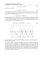
Stiffness properties of ship hull are calculated by program STIFF, based on the theory of
thin-walled girders (STIFF, 1990), Fig. 11.

Recent Advances in Vibrations Analysis

212

Fig. 11. Program STIFF – warping of ship cross-section
Influence of the transverse bulkheads is taken into account by using the equivalent torsional
modulus for the open cross-sections instead of the actual values, i.e.
*
2.4

tt
II
. This value is
applied for all ship-cross sections as the first approximation.
10.1 Analysis of ship-like segmented pontoon
Torsion of the segmented pontoon of the length L = 300 m, with effective parameters is
considered. Torsional moment M
t
= 40570 kNm is imposed at the pontoon ends. The
pontoon is considered free in the space and the problem is solved analytically according to
the formulae given in Section 4. The following values of the basic parameters are used:
10.1a  m, 19.17b  m,
1
0.01645t

m,
221
D
w


m
2
,
267
B
w

m
2

,
14.45
t
I 

m
4
,
1.894k  . As a result 22.42C

, Eq. (59), and accordingly
338.4
t
I 

m
4
, Eq. (58a), are
obtained. Since
0.36
tt
II



, effect of the short engine room structure on its torsional stiffness
is obvious.


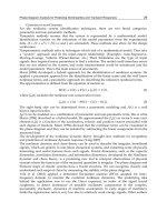
Fig. 12. Deformation of segmented pontoon, lateral and bird view

Beam Structural Modelling in Hydroelastic Analysis of Ultra Large Container Ships

213


Fig. 13. Lateral, axial, bird and fish views on deformed engine room superelement



Fig. 14. Twist angles of segmented pontoon

Recent Advances in Vibrations Analysis

214
The 3D FEM model of segmented pontoon is made by commercial software package SESAM
and consists of 20 open and 1 closed (engine room) superelement. The pontoon ends are
closed with transverse bulkheads. The shell finite elements are used. The pontoons are
loaded at their ends with the vertical distributed forces in the opposite directions,
generating total torque M
t
= 40570 kNm. The midship section is fixed against transverse and
vertical displacements, and the pontoon ends are constrained against axial displacements
(warping). Lateral and bird view on the deformed segmented pontoon is shown in Fig. 12,
where the influence of more rigid engine room structure is evident. Detailed view on this
pontoon portion is presented in Fig. 13. It is apparent that segment of very stiff double
bottom and sides rotate as a “rigid body”, while decks and transverse bulkheads are
exposed to shear deformation. This deformation causes the distortion of the cross-section,
Fig. 13.
Twist angles of the analytical beam solution and that of 3D FEM analysis for the pontoon

bottom are compared in Fig. 14. As it can be noticed, there are some small discrepancies
between

12D
ψ

and
3,Dbottom
ψ , which are reduced to a negligible value at the pontoon ends
Fig. 14 also shows twist angle of side structure and the difference
3D,bottom 3D,side
δψ ψ



represents distortion angle of cross-section which is highly pronounced. As it is mentioned
before, the problem will be further investigated.
10.2 Validation of 1D FEM model
The reliability of 1D FEM analysis is verified by 3D FEM analysis of the considered ship. For
this purpose, the light weight loading condition of dry ship with displacement Δ=33692 t is
taken into account. The equivalent torsional stiffness of the engine room structure, as well as
equivalent stiffness of fore and aft peaks is not taken into account in this example for the
time being. However, it will be done in the next step of investigation. The lateral and bird
view of the first dominantly torsional and second dominantly horizontal mode of the wetted
surface, determined by 1D model, is shown in Fig. 15.




Fig. 15. The first and second mode, lateral and bird view, light weight, 1D model

The first and second 3D dry coupled natural modes of the complete ship structure are
shown in Fig. 16. They are similar to that of 1D analysis for the wetted surface. Warping of
the transverse bulkheads, which increases the hull torsional stiffness, is evident.

Beam Structural Modelling in Hydroelastic Analysis of Ultra Large Container Ships

215
The first four corresponding natural frequencies obtained by 1D and 3D analyses are
compared in Table 1.

Mode
no.
Vert. Horiz. + tors.
Mode no.
1D 3D 1D 3D
1 7.35 7.33 4.17 4.15 1(H0 + T1)
2 15.00 14.95 7.34 7.40 2(H1 + T2)
3 24.04 22.99 12.22 12.09 3(H2 + T3)
4 35.08 34.21 15.02 16.22 4(H3 + T4)

Table 1. Dry natural frequencies, light weight, ω
i
[rad/s]



Fig. 16. The first and second mode, lateral and bird view, light weight, 3D model
Quite good agreement is achieved. Values of natural frequencies for higher modes are more
difficult to correlate, since strong coupling between global hull modes and local
substructure modes of 3D analysis occurs.

10.3 Hydroelastic response of large container ship
Transfer functions of torsional moment and horizontal bending moment at the midship
section, obtained using 1D structural model, are shown in Figs. 17 and 18, respectively. The
angle of 180
° is related to head sea. They are compared to the rigid body ones determined by
program HYDROSTAR. Very good agreement is obtained in the lower frequency domain,
where the ship behaves as a rigid body, while large discrepancies occur at the resonances of
the elastic modes, as expected.

Recent Advances in Vibrations Analysis

216

Fig. 17. Transfer function of torsional moment, χ=120°, U=25 kn, x=155.75 m from AP


Fig. 18. Transfer function of horizontal bending moment, χ=120°, U=25 kn, x=155.75 m from
AP
11. Conclusion
Ultra large container ships are quite elastic and especially sensitive to torsion due to large
deck openings. The wave induced response of such ships should be determined by using
mathematical hydroelastic models which are consisted of structural, hydrostatic and
hydrodynamic parts.
In this chapter the methodology of ship hydroelastic analysis is briefly described, and the
role of structural model is discussed. After that, full detail description of the sophisticated
beam structural model, which takes shear influence on torsion, as well as contribution of
transverse bulkheads and engine room structure to the hull stiffness, is given. Numerical
procedure for vibration analysis is also described and determination of ship cross-section

Beam Structural Modelling in Hydroelastic Analysis of Ultra Large Container Ships

217
properties is explained. The developed theories are illustrated through the numerical
examples which include analysis of torsional response of a ship-like segmented pontoon,
free vibration analysis of a large container ship and comparison with the results obtained
using 3D FEM model, and complete global hydroelastic analysis of a container ship.
It is shown that the used sophisticated beam model of ship hull, based on the advanced
thin-walled girder theory with included shear influence on torsion and a proper
contribution of transverse bulkheads and engine room structure to its stiffness, is a
reasonable choice for determining wave load effects. However, based on the experience,
stress concentration in hatch corners calculated directly by the beam model is
underestimated. This problem can be overcome by applying substructure approach, i.e.
3D FEM model of substructure with imposed boundary conditions from beam response.
In any case, 3D FEM model of complete ship is preferable from the viewpoint of
determining stress concentration. Concerning further improvements of the beam model,
the distortion induced by torsion is of interest.
The illustrative numerical example of the 7800 TEU container ship shows that the developed
hydroelasticity theory, utilizing sophisticated 1D FEM structural model and 3D
hydrodynamic model, is an efficient tool for application in ship hydroelastic analyses. The
obtained results point out that the transfer functions of hull sectional forces in case of
resonant vibration (springing) are much higher than in resonant ship motion.
12. Acknowledgment
This investigation is carried out within the EU FP7 Project TULCS (Tools for Ultra Large
Container Ships) and the project of Croatian Ministry of Science, Education and Sports Load
and Response of Ship Structures.
13. Appendix A – consistent finite element properties (frequency dependent
formulation)
The stiffness and mass matrices, Eqs. (37), are expressed with one or two integrals, which
can be classified in three different types. For general notation of shape functions



, 1,2,3,4; 0,1,2,3
k
iik
ggξ ik,

(A1)
where
ik
q
are coefficients and
/xl


, one finds the solutions of integrals in the following
form:







0
00
00 10 01 20 11 02
03 12 21 30 13 22 31
,d d
11

23
11
+
45
1
+
ll
kk
ij ik jk i j ik jk
ij ij ij ij ij ij
ij ij ij ij ij ij ij
Igg ggxg ξξ xg
lgg gg gg gg gg gg
gg gg gg gg gg gg gg


  

  


23 32 33
1
67
ij ij ij
gg gg gg






(A2)

Recent Advances in Vibrations Analysis

218






1
1k-1
00
11 12 21 13 31
22 23 32 33
d
d
,d d
dd
1

43 9
+
32 5
ll
j
k

i
i
j
ik
j
kik
j
k
ij ij ij ij ij
ij ij ij ij
g
g
Igg xg kξ kξ xg
xx
gg gg gg gg gg
l
gg gg gg gg



 







(A3)








2
2
2
22
22
00
22 23 32 33
3
d
d
,d11d
dd
43
3 .
2
ll
j
kk
i
i
j
ik
j

kik
j
k
ij ij ij ij
g
g
Igg xg kk ξ kk ξ x
g
xx
gg gg gg gg
l








(A4)
Thus, the finite element properties can be written in the following systematic way suitable
for coding.
Stiffness matrices
















21
21
1
,,
,,
,
b ij ik jk s ij ik jk
bs
w ij ik jk s ij ik jk
ws
tij ikjk
t
kEIIaa GAIbb
kEIIddGIIee
kGIIdd

 




 


 




 






(A5)
Mass matrices













01
01

0
,,
,,
,,
ij ik jk b ij ik jk
sb
t ij ik jk w ij ik jk
tw
T
cij ikjk
st ts st
mmIcc JIaa
mJIff JIdd
mmIcf m m

 




 

 




 



  
  


(A6)
Load vectors



0012310123
0012310123
111 1111
234 2345
111 1111
234 2345
iiii iiii
iiii iiii
qlqccccqcccc
μ l μ ffffμ ffff


 



 
 




 



 
 


(A7)
14. Appendix B – simplified finite element properties, from appendix A
(frequency independent formulation)
Stiffness matrices:


 

22
3
2
63 63
21 3 3 1 6
2
63
112
.213
b
bs
ll
β
ll β l

EI
k
l
β l
Sym
β
l























(B1)

Beam Structural Modelling in Hydroelastic Analysis of Ultra Large Container Ships

219


 

22
3
2
63 63
21 3 3 1 6
2
63
112
.213
w
ws
ll
γ ll γ l
EI
k
l
γ l
Sym γ l
























(B2)


 





22 22

2
22
36 3 1 60 36 3 1 60
4 1 15 360 3 1 60 1 60 720
36 3 1 60
30 1 12
. 4 1 15 360
t
t
γ l γ l
γγ
l
γ
l
γγ
l
GI
k
γ l
γ l
Sym
γγ
l






   


















(B3)

Mass matrices:

sb s b
mmm





(B4)






 


22 2 2
22 2 22
2
22
22
156 3528 20160 22 462 2520 54 1512 10080 13 378 2520
4 84 504 13 378 2520 3 84 504
156 3528 20160 22 462 2520
420 1 12
.484504
s
ββ ββ
l
ββ ββ
l
ββl ββl ββl
ml
m
ββ ββ
l
β
Sym ββl
 

   
 
 
   
 


 

 

 
 
 

 

(B5)



 





22 22
2
22

36 3 180 36 3 180
4 60 1440 3 180 1 60 720
36 3 180
30 1 12
. 4 60 1440
b
b
β l β l
ββ
l
β
l
ββ
l
J
m
β l
β l
Sym
ββ
l







  




















(B6)


tw t w
mmm





(B7)






 


22 2 2
22 2 22
2
22
22
156 3528 20160 22 462 2520 54 1512 10080 13 378 2520
4 84 504 13 378 2520 3 84 504
156 3528 20160 22 462 2520
420 1 12
. 4 84 504
t
t
γγ γγ
l
γγ γγ
l
γγl γγl γγl
Jl
m
γγ γγ
l
γ

Sym γγl
 
   
 
 
   
 


 

 

 
 
 

 

(B8)



 





22 22

2
22
36 3 180 36 3 180
4 60 1440 3 180 1 60 720
36 3 180
30 1 12
. 4 60 1440
w
w
γ l γ l
γγl γ l γγl
J
m
γ l
γ l
Sym γγl







  




















(B9)

Recent Advances in Vibrations Analysis

220

 

2 2
420 1 12 1 12
156 1764 1764 20160 22 252 210 2520 54 756 756 10080 13 168 210 2520
22 210 252 2520 4 42 42 504 13 210 168 2520 3 42 42 504

54 7
st
mlc
m

βγ
β γ βγ β γ βγ
l
βγ βγ βγ βγ
l
βγ βγl βγ βγl βγ βγl βγ βγl




   
   

 

2 2
56 756 10080 13 168 210 2520 156 1764 1764 20160 22 252 210 2520
13 210 168 2520 3 42 42 504 22 210 252 2520 4 42 42 504
β γ βγ β γ βγ
l
β γ βγ β γ βγ
l
βγ βγl βγ βγl βγ βγl βγ βγl
 
 
 
 
 
     
 

 
       
 
 
(B10)

T
ts st
mm





(B11)
Load vectors:





01
9 120
6
230
21 240
6
12 60 1 12
330
β

β
l
l
ql ql
q
β
β
β
l
l

























(B12)





01
9 120
6
230
21 240
6
12 60 1 12
330
γ
γ l
l
μ l μ l
μ
γ
γ
γ l
l

























(B13)
Stiffness ratios:

22
, .
bw
ss
EI EI
βγ

GA l GI l


(B14)
15. References
Bathe, KJ. (1996). Finite Element Procedures, Prentice Hall
Cheung, YK. (1976). Finite Strip Method in Structural Analysis, Pergamon Press
Haslum, K. & Tonnessen, A. (1972). An Analysis of Torsion in Ship Hull, European
Shipbuilding, No.5/6, pp. 67-89
Kawai, T. (1973). The Application of Finite Element Method to Ship Structures, Computers &
Structures, Vol.3, No.5, pp. 1175-1194, ISSN 0045-7949
Lozina, Ž. (1988). A Comparison of Harmonic Acceleration Method with the Other
Commonly Used Methods for Calculation of Dynamic Transient Response,
Computers & Structures, Vol.29, No.2, pp. 227-240, ISSN 0045-7949
Pavazza, R. (1991). Bending and Torsion of Thin-Walled Beams of Open Section on Elastic
Foundation, Ph.D. Thesis. University of Zagreb, (in Croatian)
Pavazza, R. (2005). Torsion of Thin-Walled Beams of Open Cross-Sections with Influence of
Shear, International Journal of Mechanical Sciences, Vol.47, No.7, pp. 1099-1122, ISSN
0020-7403
Pedersen, PT. (1983). A Beam Model for the Torsional-Bending Response of Ships Hulls,
RINA Transactions, Vol.31, pp. 171-182

Beam Structural Modelling in Hydroelastic Analysis of Ultra Large Container Ships

221
Pedersen, PT. (1985). Torsional Response of Container Ships, Journal of Ship Research, Vol.29,
pp. 194-205, ISSN 1542-0604
Senjanović, I. (1984). Harmonic Acceleration Method for Dynamic Structural Analysis,
Computers & Structures, Vol.18, No.1, pp. 71-80, ISSN 0045-7949
Senjanović, I. (1990). Ship Vibrations, Part II, University of Zagreb, (in Croatian)

Senjanović, I. & Fan, Y. (1989). A Higher-Order Flexural Beam Theory, Computers &
Structures, Vol.32, No.5, pp. 973-986, ISSN 0045-7949
Senjanović, I. & Fan, Y. (1992). A Higher-Order Theory of Thin-Walled Girders with
Application to Ship Structures, Computers & Structures, Vol.43, No.1, pp. 31-52,
ISSN 0045-7949
Senjanović, I. & Fan, Y. (1993). A Finite Element Formulation of Initial Ship Cross-Section
Properties, Brodogradnja, Vol.41, No.1, pp. 27-36, ISSN 0007-215X
Senjanović, I. & Fan, Y. (1997). A Higher-Order Torsional Beam Theory, International Journal
for Engineering Modelling, Vol.32, No.1-4, pp. 25-40, ISSN 1330-1365
Senjanović, I. & Grubišić, R. (1991). Coupled Horizontal and Torsional Vibration of a Ship
Hull with Large Hatch Openings, Computers & Structures, Vol.41, No.2, pp. 213-226,
ISSN 0045-7949
Senjanović, I., Malenica, Š., Tomašević, S. & Rudan, S. (2007). Methodology of Ship
Hydroelastic Investigation, Brodogradnja, Vol.58, No.2, pp. 133-145, ISSN 0007-215X
Senjanović, I. , Tomašević, S., Tomić, M., Rudan, S., Vladimir N. & Malenica, Š. (2008a).
Hydroelasticity of Very Large Container Ships, Proceedings of International
Conference on Design and Operation of Container Ships, pp. 51-70, RINA, London
Senjanović, I., Tomašević, S., Rudan, S. & Senjanović, T. (2008b). Role of Transverse
Bulkheads in Hull Stiffness of Large Container Ships, Engineering Structures, Vol.30,
No.9, pp. 2492-2509, ISSN 0141-0296
Senjanović, I., Tomašević, S. & Vladimir, N. (2009a). An Advanced Theory of Thin-Walled
Girders with Application to Ship Vibrations, Marine Structures, Vol.22, No.3, pp.
387-437, ISSN 0951-8339
Senjanović, I. , Tomašević, S., Vladimir N. & Malenica, Š. (2009b). Numerical Procedure for
Ship Hydroelastic Analysis,
Proceedings of International Conference on Computational
Metho
ds in Marine Engineering, pp. 259-264, CIMNE, Barcelona
Senjanović, I., Vladimir, N. & Tomić, M. (2010a). The Contribution of the Engine Room
Structure to the Hull Stiffness of Large Container Ships, International Shipbuilding

Progress, Vol.57, No.1-2, pp. 65-85, ISSN 0020-868X
Senjanović, I. , Tomašević, S., Vladimir N. Tomić, M. & Malenica, Š. (2010b). Application of
an Advanced Beam Theory to Ship Hydroelastic Analysis, Proceedings of
International Workshop on Advanced Ship Design for Pollution Prevention, pp. 31-42,
Taylor & Francis, London
STIFF (1990). User's Manual, University of Zagreb
Szilard, R. (2004). Theories and Applications of Plate Analysis, John Wiley & Sons, New York
Timoshenko, S. & Young, DH. (1955). Vibrations Problems in Engineering, D. Van Nostrand
Tomašević, S. (2007). Hydroelastic Model of Dynamic Response of Container Ship in Waves, Ph.D.
Thesis. University of Zagreb, (in Croatian)

Recent Advances in Vibrations Analysis

222
Vlasov, VZ. (1961). Thin-Walled Elastic Beams, Israel Program for Scientific Translation,
Jerusalem
Wu, YS. & Ho, CS. (1987). Analysis of Wave Induced Horizontal and Torsion Coupled
Vibrations of Ship Hull. Journal of Ship Research, Vol.31, No.4, pp. 235-252, ISSN
1542-0604
11
Stochastic Finite Element Method in
Mechanical Vibration
Mo Wenhui
Hubei University Of Automotive Technology
China
1. Introduction
Material properties, geometry parameters and applied loads of the structure are assumed to
be stochastic. Although the finite element method analysis of complicated structures has
become a generally widespread and accepted numerical method in the world, regarding the
given factors as constants can not apparently correspond to the reality of a structure.

The direct Monte Carlo simulation of the stochastic finite element method(DSFEM) requires
a large number of samples, which requires much calculation time and occupies much
computer storage space [1]. Monte Carlo simulation by applying the Neumann expansion
(NSFEM) enhances computational efficiency and saves storage in such a way that the
NSFEM combined with Monte Carlo simulation enhances the finite element model
advantageously [2]. The preconditioned Conjugate Gradient method (PCG) applied in the
calculation of stochastic finite elements can also enhance computational accuracy and
efficiency [3]. The TSFEM assumes that random variables are dealt with by Taylor
expansion around mean values and is obtained by appropriate mathematical treatment [4,
14]. According to first-order or second-order perturbation methods, calculation formulas can
be obtained [2, 5, 6,8, 9, 13, 15, 16]. The result is called the PSFEM and has been adopted by
many scholars.
The PSFEM is often applied in dynamic analysis of structures and the second- order
perturbation technique has been proved to be accurate and efficient. Dynamic reliability of a
large frame is calculated by the SFEM and response sensitivity is formulated in the context
of stiffness and mass matrix condensation [7]. Nonlinear structural dynamics are developed
by the PSFEM. Nonlinearities due to material and geometrical effects have also been
included [8]. By forming a new dynamic shape function matrix, dynamic analysis of the
spatial frame structure is presented by the PSFEM [9].
It is significant to extend this research to the dynamic state. Considering the influence of
random factors, the mechanical vibrations for a linear system are illustrated by using the
TSFEM and the CG.
2. Random variable
Material properties, geometry parameters and applied loads of machines are assumed to be
independent random variables, and are indicated as
12
,,,aa
1
,,
in

aa . Their means
are
1
12
, ,,,,
in


 , and their variances are
1
22
,,
in

 . When they are subject to

Recent Advances in Vibrations Analysis

224
normal distributions, the standard method used to simulate them is to take advantage of
well-tested computer programs. When they are subject to unknown distributions, the
sample of
1
12
,,,,,
in
aa a a can be generated from the following method:


2

2
Px




 (1)
where,
x is a random variable,


is the mean,

is the standard deviation ,and

is an
arbitrary positive number. Eq.1 is called the Chebyschev inequality.
The Chebyschev inequality can also be written as


2
2
1Px





(2)
After substituting

6
i



,
i
xa

, Eq.2 becomes



6 0.9722
ii i
Pa

  (3)
where
6
iii
a



 (4)
or

6
iii

a


 
(5)
If it is assumed that z

is a random number within the open interval (0,1), then

6
iii
az




 (6)
or

6
iii
az




 (7)
Large numbers of samples of random variables
1
12

,,,,,
in
aa a a are produced from Eqs.6
and 7 so as to resolve the stochastic finite element problem through Monte Carlo
stimulation.
3. Dynamic analysis of finite element
For a linear system, the dynamic equilibrium equation is given by















M
CK F


 
(8)
where







,,


 
are the acceleration, velocity and displacement vectors.




,
M
K and


C are the global mass, stiffness and damping matrices obtained by assembling the element
variables in global coordinate system.
In order to program easily, the comprehensive calculation steps of the Newmark method are
as follows

Stochastic Finite Element Method in Mechanical Vibration

225
1. The initial calculation
The matrices



K
,


M
and


C
are formed.
The initial values






,,
ttt



are given.
After selecting step t

and parameters ,


, the following relevant parameters are

calculated:
0.50



2
0.25 0.5




0
2
1
b
t




1
b
t





2
1

b
t




3
1
1
2
b



4
1b




5
2
2
t
b












6
1bt



7
bt



The stiffness matrix is defined as







01
KKbMbC


 




(9)
The stiffness matrix inversion
1
K






is solved.
2.
Calculation of each step time
At time tt , the load vector is defined as









0tt tt t
FFMb

 









23tt
bb
















145ttt
Cb b b





(10)
At time
tt , the displacement vector is given by




1
tt tt
KF


 





(11)
At time
tt , the velocity vector and acceleration vector are obtained as














023tt tt t t t
bbb

 
 

  
(12)









67tt t t tt
bb

 
 

(13)
Vectors







111
,,
ti t ti t ti t

  

are solved at time


11 3
2,3, ,titi n   step-by -step.
4. Analysis of mechanical vibration based on CG
Eq.11 can be expressed as




tt tt
KF








(14)

Recent Advances in Vibrations Analysis

226
1
N samples of random variables
1
12
,,,,,
in
aa a a are produced.
1
N matrices K



and
1
N
Eqs.14 are also generated. For a linear vibration, Eq.14 is the system of linear equations. The
CG method is an effective method for solving the large system of linear equations according
to the following steps:
1.
First, select an approximate solution as the initial value

 








12
000 0
,,,
N
T
tt
tt tt tt
 


  
  (15)
2.
Calculate the first residual vector







00
tt tt
rF K








(16)
and vector

 
00
T
p
Kr




(17)
where,
T
K



is the transposed matrix of K







3.
For
2
0,1,2, , 1in


, iterate step-by-step as follows

 
 
 
 
 
 
,, ,
,, ,
TTT
ii ii ii
i
ii ii ii
Kpr p Kr Kr Kr
Kp Kp Kp Kp Kp Kp

  
   
  
   

  


     

     

  

  

  
(18)






1
i
ii
tt tt
i
p


 





(19)

   
1ii i
i
rr Kp





 


(20)

 
 
11
1
,
,
TT
ii
i
TT
ii
Kr Kr

Kr Kr




 

 



 

 






(21)

  
11
1
T
iii
i
p
Kr p










(22)
The process can be stopped only if
2
n
r is small enough.
Vectors






1
12
,,,
tt tt tt
N
 
  
 are solutions of
1

N Eqs.14.
The mean of


tt


is given by








1
12
1
tt tt tt
N
tt
N
 

  





(23)

Stochastic Finite Element Method in Mechanical Vibration

227
The variance of


tt


is given by

 

1
2
1
1
1
1
N
tt tt tt
i
i
Var
N

  





(24)
Similarly, the mean and variance of the vector


1
ti t



can be solved for at
time


11 3
2,3, ,titi n  
step-by-step.
At time


22 4
1,2, ,ttiti n

   ,the strain and stress vectors for element d are






d
t
B



(25)
and





D



(26)
where,


D
=the material response matrix of element d ,


B
=the gradient matrix of
element
d and



d
t


=the element d nodal displacement vector at time t

.
Substituting Eq.25 into Eq.26, the stress for element
d is given by





d
t
DB



(27)
Substituting samples of random variables
1
12
,,,,,
in
aa a a into Eq.27, the vectors







1
12
,,,
N
 
 can be obtained.
The mean of



is given by


  
1
12
1
N
N
 




(28)

The variance of



is given by

  

1
2
1
1
1
1
N
i
i
Var
N





(29)
The CG method belongs to method of iteration with the advantage of quick convergence.
For practical purpose, PCG is applied to accelerate the convergence.
5. Analysis of mechanical vibration based on TSFEM
Independent random variables of the system are regarded as
1

12
,,,,,
in
aa a a .
The partial derivative of Eq.14 with respect to
i
a
is given by





1
tt
tt
tt
iii
F
K
K
aaa























(30)

Recent Advances in Vibrations Analysis

228
where









023

tt
tt
tt t
ii iii
F
F
Mb b b
aa aaa












 







 


023ttt
i
M
bbb
a
















 

145
145
tt
t
iii
ttt
i

Cb b b
aaa
C
bbb
a
















(31)

After





00 00 00

,,
tt
t
ttt
iii
qqq
aaa









are given, Eq.31 can be calculated.
The partial derivative of Eq.30 with respect to
i
a is given by


2
1
2
tt
i
K
a















2
2
22
2{}
tt
tt
tt
ii
ii
F
KK
aa
aa







 



 








(32)
where





 

2
22
023
222
tt
tt

ttt
iii
F
F
M
bbb
aaa


















023
2
tt
t
ii i i

M
bbb
aa a a








  








22
2
023
222
tt
t
iii
Mb b b
aaa
















 









 
2
145 1 4 5
2
22
2

145
222
2
tt
t
ttt
ii i i
i
tt
t
iii
CC
bbb b b b
aa a a
a
Cb b b
aaa










 

  














(33)
After





22
2
00 00 00
222
,,
tt
t
ttt
iii
rrr

aaa









are given, Eq.33 can be calculated.
The displacement is expanded at the mean value point

1
12
,,,,,
T
in
aaa a a  by means of
a Taylor series. By taking the expectation operator for two sides of above Eq.11, the mean of
the displacement is obtained as