Vibration Analysis and Control New Trends and Developments Part 2 potx
Bạn đang xem bản rút gọn của tài liệu. Xem và tải ngay bản đầy đủ của tài liệu tại đây (2.72 MB, 25 trang )
Adaptive Tuned Vibration Absorbers: Design Principles, Concepts and Physical Implementation
15
High accuracy is guaranteed here by solving the frequencies
a
ω
,
m
ω
for 39K = , which
means that 20 symmetric free-free plain beam flexural modes were considered.
Now, for the equivalent two-degree-of-freedom system in Fig. 1b, one can write the
attachment point receptance as (Kidner & Brennan, 1997):
()
()
{}
22
2-DOF
22 2
,,,
1
a
AA
ared ae
ff
ared a
r
mmm
ωω
ω
ω
ωω
−
=
−+
(15)
where
,ae
ff
a
mRm
=
,
(
)
,
1
a red a
mRm=− ,
(
)
1
ab
mm
σ
=+ (16a-c)
The non-zero resonance of the function in eq. (15) is given by:
,,
2-DOF
1
maae
ff
ared
mm
ωω
=+ (17)
For equivalence,
2-DOF
mm
ω
ω
= in eq. (17). Hence, by substituting this condition and eqs.
(16a,b) into eq. (17), an expression can be obtained for the proportion R of the total absorber
mass
a
m that is effective in vibration attenuation:
()
()
2
,1
am
Rx
σωω
=−
(18)
…where
a
ω
,
m
ω
are the roots of eqs. (12, 13). Also, from eq. (15) and eqs. (16), the non-
dimensional attachment point receptance of the equivalent system can be written as:
() ()
()()
{}
22
2
1
222
2-DOF 2-DOF
,,
11
a
AA b AA
a
rx mr
R
ωω
ωσ ω ω
σ
ωωω
−
==
+−−
(19)
The equivalent two-degree-of-freedom model is verified in Fig. 17 against the exact theory
governing the actual (continuous) ATVA structures of Fig. 16 for 5
σ
=
and two given
settings 0.25
x =
, 0.5 . For each setting of
x
the corresponding values of
a
ω
and R were
calculated using eqs. (12, 13, 18) and used to plot the function
(
)
2-DOF
,,
AA
rx
ωσ
in eq. (19).
Comparison with the exact receptance
(
)
,,
AA
rx
ω
σ
(computed from eqs. (9) and (11)) shows
that the equivalent two-degree-of-freedom system is a satisfactory representation of the
actual systems in Fig. 16 over a frequency range which contains the operational frequency of
the ATVA (
a
ω
ω
= ).
Next, using eqs. (12, 13, 18), the variations of
a
ω
and R with ATVA setting x
for various
fixed values of
σ
are investigated for both types of ATVA in Fig. 16. The resulting
characteristics are depicted in Fig. 18. With reference to Fig. 18a, it is evident that, as
σ
is
increased, the tuning frequency characteristics of both types of ATVA approach each other.
Moreover, for 1
σ
≥ , both types of ATVA give roughly the same overall useable variation in
a
ω
relative to
1
a
x
ω
=
. The moveable-supports ATVA characteristics in Fig. 18a have a peak
(which is more prominent for lower
σ
values) that gives the impression of a greater
variation in
a
ω
than the moveable-masses ATVA. However, this is a “red herring” since
Vibration Analysis and Control – New Trends and Developments
16
these peaks coincide with a stark dip to zero in the effective mass proportion R of the
moveable-supports ATVA, as can be seen in Fig. 18b. These troughs in
R are explained by
the fact that, for given
σ
, the free body resonance
m
ω
of the moveable-supports ATVA (i.e.
the resonance of the free-free beam with central mass attached) is fixed (i.e. independent of
x
), as can be seen from Figs. 17c,d. Hence, the nodes of the associated mode-shape are fixed
in position so that when the setting
x
is such that the attachment points A of the moveable-
supports ATVA coincide with these nodes, this ATVA becomes totally useless (i.e.
attenuation 0
D = , eq. (7)).
Fig. 17. Verification of equivalent two-degree-of-freedom model - non-dimensional
attachment point receptance plotted against non-dimensional excitation frequency for two
settings of the ATVAs in Figure 3 with 5
σ
=
: exact, through eqs. (9) and (11) (――――);
equivalent 2-degree-of-freedom model, from eq. (19 ) (▪▪▪▪▪▪▪▪▪)
The moveable-masses ATVA does not suffer from this problem, and consequently has vastly
superior effective mass characteristics, as evident from Fig. 18b. From eqs. (16a, b), one can
rewrite the attenuation
D in eq. (8) as:
Adaptive Tuned Vibration Absorbers: Design Principles, Concepts and Physical Implementation
17
1
1
aa
R
D
RMm
η
⎛⎞
=
⎜⎟
−+
⎝⎠
(20)
It is evident from Fig. 18b and eq. (20) that the degree of attenuation D provided by a given
moveable-supports ATVA in any given application undergoes considerable variability over
its tuning frequency range, dipping to zero at a critical tuned frequency. On the other hand,
the moveable-masses ATVA can be tuned over a comparable tuning frequency range while
providing significantly superior vibration attenuation.
Fig. 18. Tuned frequency and effective mass characteristics for moveable-masses ATVA
Vibration Analysis and Control – New Trends and Developments
18
4.2 Physical implementation and testing
Fig. 19 shows the moveable-masses ATVA with motor-incorporated masses that was built in
(Bonello & Groves, 2009) to lend validation to the theory of the previous section and
demonstrate the ATVA operation. The stepper-motors were operated from the same driver
circuit board through a distribution box that sent identical signals to the motors, ensuring
symmetrically-disposed movement of the masses. Each motor had an internal rotating nut
that moved it along a fixed lead-screw. Each motor was guided by a pair of aluminium
guide-shafts that, along with the lead-screw, made up the beam section.
The aim of Section 4.2.1 is to validate the theory of Section 4.1 whereas the aim of Section
4.2.2 is to demonstrate real-time ATVA operation.
4.2.1 Tuned frequency and effective mass characteristics
In these tests a random signal
v
was sent to the electrodynamic shaker amplifier and for
each fixed setting
x
the frequency response function (FRF)
Av
H relating
A
y
to
v
, and the
FRF
BA
T relating
B
y
to
A
y
(i.e. the transmissibility) were measured. Fig. 20a shows
Av
H
for different settings. The tuned frequency
a
ω
of the ATVA is the anti-resonance, which
coincides with the resonance in
BA
T . Fig. 20b shows that, at the anti-resonance, the cosine of
the phase of
BA
T is approximately zero. This is an indication that the absorber damping
a
η
(Fig. 1b) is low (Kidner et al., 2002). Hence, just like other types of ATVA e.g. (Rustighi et.
al., 2005, Bonello et al., 2005, Kidner et al., 2002), the cosine of the phase
Φ
between the
signals
A
y
and
B
y
can be used as the error signal of a feedback control system for the
ATVA under variable frequency harmonic excitation (Section 4.2.2). It is noted that this
result is in accordance with the two-degree-of-freedom modal reduction of the ATVA and,
additionally, it could be shown theoretically that the cosine of the phase between
A
y
and
the signal
Q
y
at any other arbitrary point Q on the ATVA would also be zero in the tuned
condition.
Fig. 19. Moveable-masses ATVA demonstrator mounted on electrodynamic shaker (inset
shows motor-incorporated mass and ATVA beam cross-section)
Adaptive Tuned Vibration Absorbers: Design Principles, Concepts and Physical Implementation
19
Using the FRFs of Fig. 20a and a lumped parameter model of the ATVA/shaker
combination it was possible to estimate the effective mass proportion
R of the ATVA for
each setting
x
, using the analysis described in (Bonello & Groves, 2009). The estimates
varied slightly according to the type of damping assumed for the shaker armature
suspension. However, as can be seen in Fig. 21, regardless of the damping assumption, there
is good correlation with the effective mass characteristic predicted according to the theory of
the previous section. Fig. 22 shows the predicted and measured tuning frequency
characteristic, which gives the ratio of the tuned frequency to the tuned frequency at a
reference setting. The demonstrator did not manage to achieve the predicted 418 % increase
in tuned frequency, although it managed a 255 % increase, which is far higher than other
proposed ATVAs e.g. (Rustighi et. al., 2005, Bonello et al., 2005, Kidner et al., 2002) and
similar to the percentage increase achieved by the V-Type ATVA in (Carneal et al., 2004).
The main reasons for a lower-than-predicted tuned frequency as
x
was reduced can be
listed as follows: (a) the guide-shafts-pair and lead-screw constituting the “beam cross-
section” (Fig. 19) would only really vibrate together as one composite fixed-cross-section
beam in bending, as assumed in the theory, if their cross-sections were rigidly secured
relative to each other at regular intervals over the entire beam length – this was not the case
in the real system and indeed was not feasible; (b) shear deformation effects induced by the
inertia of the attached masses at B and the reaction force at A became more pronounced as
x
was reduced; (c) the slight clearance within the stepper-motors. It is noted that the
limitation in (a) was exacerbated by the offset of the centroidal axis of the lead-screw from
that of the guide-shafts (inset of Fig. 19). Moreover, the limitations described in (a) and (b)
are also encountered when implementing the moveable-supports design (Fig. 16b). It is also
interesting to observe that, at least for the case studied, the divergence in Fig. 22 did not
significantly affect the good correlation in Fig. 21.
4.2.2 Vibration control tests
Fig. 23 shows the experimental set-up for the vibration control tests. The shaker amplifier
was fed with a harmonic excitation signal
v of time-varying circular frequency
ω
and fixed
amplitude and the ability of the ATVA to attenuate the vibration
A
y
by maintaining the
tuned condition
a
ω
ω
=
in real time was assessed. The frequency variation occurred over the
interval
i
f
ttt<< and was linear:
()()
()
i
i
i
f
i
f
iii
f
f
f
tt
tt tt ttt
tt
ω
ωω ωω
ω
⎧
≤
⎪
⎪
⎡⎤
=
+− − − <<
⎨
⎣⎦
⎪
⎪
≥
⎩
(21)
where
i
ω
,
f
ω
are the initial and final frequency values. The swept-sine excitation signal
was hence as given by:
sin
vV
θ
=
,
d
dt
θ
ω
=
(22a,b)
Vibration Analysis and Control – New Trends and Developments
20
where, by substitution of (21) into (22b) and integration:
()()
()
()()
2
0.5
0.5
i
i
f
i
f
iiii
f
f
ffifi
t
tt
tt tt t ttt
tt
ttt
ω
θωω ω
ωωω
⎧
⎪
≤
⎪
⎪
⎡⎤
=
−−−+ <<
⎨
⎣⎦
⎪
⎪
≥
⎡⎤
−−+
⎪
⎣⎦
⎩
(23)
Fig. 20. Frequency response function measurements for different settings of ATVA of Fig. 19
The inputs to the controller were the signals
A
y
,
B
y
from the accelerometers. As discussed
in Section 4.2.1, the instantaneous error signal fed into the controller was
(
)
coset =Φ
and
this was continuously evaluated from
A
y
,
B
y
by integrating their normalised product over
a sliding interval of fixed length
c
T , according to the following formula:
Adaptive Tuned Vibration Absorbers: Design Principles, Concepts and Physical Implementation
21
()
(
)
()
{}
()
{}
()
()
()
()
()
{}
()
()
{}
()
0.5 0.5
0.5 0.5
cos
AB
c
AA BB
AB AB c
c
AA AA c BB BB c
It
tT
It It
et
ItItT
tT
ItItT ItItT
⎧
≤
⎪
⎪
⎪
=Φ=
⎨
⎪
−−
⎪
>
⎪
−− −−
⎩
(24)
where
() () ()
0
t
AA A A
It y y d
τ
ττ
=
∫
,
() () ()
0
t
BB B B
It y y d
τ
ττ
=
∫
,
() () ()
0
t
AB A B
It y y d
τ
ττ
=
∫
(25a-c)
…and
c
T was taken to be many times the interval
Δ
between consecutive sampling times of
the data acquisition (
100
c
T
=
Δ typically). Since the difference between the forcing
frequency and the tuned frequency,
a
ω
ω
−
is non-linearly related to
(
)
et
, a non-linear
control algorithm was necessary to minimise
(
)
et . Various such control algorithms for
ATVAs have been proposed. For example, (Bonello et al., 2005) used a nonlinear P-D
controller in which the voltage that controlled the piezo-actuators (Fig. 10) was updated
according to a sum of two polynomial functions, one in
e
and the other in e
, weighted by
suitably chosen constants P and D. (Kidner et al., 2002) formulated a fuzzy logic algorithm
based on
e
to control the servo-motor of the device in Figure 12b. These algorithms were
not convenient for the present application since they provided an analogue command signal
to the actuator. In the present case, the available motor driver was far more easily operated
through logic signals. Each motor had five possible motion states, respectively activated by
five possible logic-combination inputs to the driver. Hence, the interval-based control
methodology described in Table 1 was implemented, where the error signal computed by
eq. (24) was divided into 5 intervals.
Fig. 21. Effective mass characteristics for prototype moveable masses ATVA: predicted
(▪▪▪▪▪▪▪); measured, light damping assumption (――■――); measured, proportional damping
assumption (――▼――)
Vibration Analysis and Control – New Trends and Developments
22
Fig. 22. Tuned frequency characteristic for prototype moveable masses ATVA: predicted
(▪▪▪▪▪▪▪); measured (――■――)
Fig. 23. Experimental set-up for vibration control test
The control system for the experimental set-up of Figure 23 was implemented in MATLAB
®
with SIMULINK
®
using the Real Time Workshop
®
and Real Time Windows Target
®
toolboxes.
Fig. 24 shows the results obtained for the frequency-sweep in Fig. 24a with the control
system turned off and the ATVA tuned to a frequency of 56Hz. It is clear that at the instant
in
p
ut
/
out
p
u
t
motor
driver
electrodynamic
shaker
PC running
Simulink ®
variable frequency
harmonic excitation
signal
B
y
logic output from Simulink®
controller
distribution
box
A
y
accelerometers
mass incorporating
stepper motor
B
B
A
amplifier
am
p
lifier
Adaptive Tuned Vibration Absorbers: Design Principles, Concepts and Physical Implementation
23
where the excitation frequency sweeps through 56 Hz, the amplitude of the acceleration
A
y
is at a minimum value and
cos
Φ
is approximately equal to zero (i.e. the ATVA is
momentarily tuned to the excitation).
Fig. 24. Swept-sine test with controller turned off and ATVA tuned to a fixed frequency of
56 Hz (
peak
A
y
is the amplitude of
A
y
, the tuned acceleration at A at an excitation
frequency of 56 Hz)
Vibration Analysis and Control – New Trends and Developments
24
cos
Φ
Motion State
1
cos 1c
Φ
≤
≤
Fast CW
21
coscc
Φ
≤
<
Slow CW
22
coscc
Φ
−
<<
Stopped
21
coscc
Φ
−
≥>−
Slow CCW
1
cos 1c
Φ
−
≥≥−
Fast CCW
Table 1. Interval-based control methodology for stepper-motor driver (CW: clockwise;
CCW: counter-clockwise)
Fig. 25. Response to swept sine excitation (Figure 24a) with controller turned on and ATVA
initially tuned to the excitation frequency (controller parameters in Table 1 are
1
0.04c = , 02.0
2
=c ).
Fig. 25 shows the response to the same frequency-sweep of Fig. 24a with the controller turned
on. Prior to the start of the frequency-sweep at 10t
=
, the ATVA was allowed to tune itself,
from whatever initial setting it had, to the prevailing excitation frequency of 30 Hz. As the
sweep progressed, the controller retuned the ATVA accordingly to reasonable accuracy, as
illustrated in Fig. 25b. This resulted in minimised vibration over the entire sweep, as evident
by comparing the scales of the vertical axes of Fig. 25a and 24b. However, it is evident from
Adaptive Tuned Vibration Absorbers: Design Principles, Concepts and Physical Implementation
25
Fig. 25a that the amplitude of the tuned vibration increases steadily over the frequency sweep
between start and finish. Further studies revealed that this observed degradation in
attenuation produced by the ATVA was due to the reduction in its effective mass proportion R
as it retuned itself to a higher frequency, decreasing the effective mass ratio
μ
of the ATVA-
shaker combination. This illustrated the importance of knowing the effective mass
characteristic of a moveable-masses or moveable-supports ATVA. It is noted that the tests in
this subsection (4.2.2) were made with an earlier version of the prototype wherein the ATVA
beam came in two halves i.e. one separate lead-screw and a separate guide-shaft-pair for each
symmetric half of the ATVA, each secured into the central block (see Fig. 19). The tests in
section 4.2.1 were made with an improved version wherein the ATVA beam was one
continuous piece, as in the theory (Fig. 16a) i.e. one long lead-screw and guide-shaft pair
running straight through the central block, where they were tightly secured, ensuring a
horizontal slope (see Fig. 19). Based on the validated results of Fig. 21, the observed
degradation in attenuation in Fig. 25a is expected to be much less for the improved version.
5. Conclusion
This chapter started with a quantitative illustration of the basic design principles of both
variants of the TVA: the TMD and the TVN. The importance of adaptive technology,
particularly with regard to the TVN, was justified. The remainder of the chapter then
focussed on adaptive (smart) technology as applied to the TVN. A comprehensive review of
the various design concepts that have been proposed for the ATVA was presented. The
latest ATVA concept introduced by the author, involving a beam-like ATVA with actuator-
incorporated moveable masses, was then studied theoretically and experimentally. The
variation in tuned frequency was shown to be significantly higher than most other proposed
ATVAs and at least as high as that reported in the literature for the alternative moveable-
supports beam ATVA design. Moreover, the analysis revealed that the moveable-masses
beam concept offers significantly superior vibration attenuation relative to the moveable-
supports beam concept, apart from constructional simplicity. Vibration control tests with
logic-based feedback control demonstrated the efficacy of the device under variable
frequency excitation. Current efforts by the author are being directed at introducing smart
technology to TMDs.
6. References
Bishop, R.E.D. & Johnson, D.C. (1960). The Mechanics of Vibration, Cambridge University
Press, Cambridge, UK
Bonello, P. & Brennan, M. J. (2001). Modelling the dynamic behaviour of a supercritical rotor
on a flexible foundation using the mechanical impedance technique. J. Sound and
Vibration, Vol.239, No.3, pp. 445-466
Bonello, P.; Brennan, M. J. & Elliott, S. J. (2005). Vibration control using an adaptive tuned
vibration absorber with a variable curvature stiffness element. Smart Mater. Struct.,
Vol.14, No.5, pp. 1055-1065
Bonello, P. & Groves, K.H. (2009). Vibration control using a beam-like adaptive tuned
vibration absorber with actuator-incorporated mass-element. Proceedings of the
Institution of Mechanical Engineers - Part C: Journal of Mechanical Engineering
Science.,Vol.223.,No.7, pp 1555-1567
Vibration Analysis and Control – New Trends and Developments
26
Brennan, M.J. (1997). Vibration control using a tunable vibration neutraliser. Proc. IMechE
Part C, Journal of Mechanical Engineering Science, Vol.211, pp. 91-108
Brennan, M.J. (2000). Actuators for active control – tunable resonant devices. Applied
Mechanics and Engineering, Vol.5, No.1, pp. 63-74
Brennan, M.J.; Bonello, P.; Rustighi, E., Mace, B.R. & Elliott, S.J. (2004a). Designs of a variable
stiffness element for a tunable vibration absorber, Proceedings of ICA2004 (The 18th
International Congress on Acoustics), Vol.IV, pp. 2915-2918, Kyoto, Japan, 4-9
April , 2004
Brennan, M.J.; Bonello, P.; Rustighi, E., Mace, B.R. & Elliott, S.J. (2004b). Designs of a
variable stiffness element for a tunable vibration absorber, Presentation given at
ICA2004 (The 18th International Congress on Acoustics), Vol.IV, pp. 2915-2918, Kyoto,
Japan, 4-9 April , 2004
Carneal, J.P.; Charette, F. & Fuller, C.R. (2004). Minimization of sound radiation from plates
using adaptive tuned vibration absorbers. J. Sound and Vibration, Vol.270, pp.
781-792
Den Hartog, J.P. (1956). Mechanical Vibrations, McGraw Hill (4
th
Edition), New York, USA
Ewins, D.J. (1984). Modal Testing: Theory and Practice, Letchworth: Research Student
Press, UK
Hong, D.P. & Ryu, Y.S. (1985). Automatically controlled vibration absorber. US Patent No.
4935651
Kidner, M.R.F. & Brennan, M.J. (1999). Improving the performance of a vibration neutraliser
by actively removing damping. J. Sound and Vibration, Vo.221, No.4, pp. 587-606
Kidner, M. R. F. & Brennan, M. J. (2002). Variable stiffness of a beam-like neutraliser under
fuzzy logic control. Trans. of the ASME, J. Vibration and Acoustics, Vol.124, pp. 90-99
Ormondroyd, J. & den Hartog, J.P. (1928). Theory of the dynamic absorber. Trans. of the
ASME, Vol. 50, pp. 9-22
Long, T.; Brennan, M.J. & Elliott, S.J. (1998). Design of smart machinery installations to
reduce transmitted vibrations by adaptive modification of internal forces.
Proceedings of the Institution of Mechanical Engineering - Part I: Journal of Systems and
Control Engineering, Vol.212, No.13, pp. 215-228
Longbottom, C.J.; Day M.J. & Rider, E. (1990). A self tuning vibration absorber. UK Patent
No. GB218957B
Park, C.H. (2003). Dynamics modelling of beams with shunted piezoelectric elements. J.
Sound and Vibration, Vol.268, pp. 115-129
Rustighi, E.; Brennan, M.J. & Mace, B.R. (2005). A shape memory alloy adaptive tuned
vibration absorber: design and implementation. Smart Mater. Struct., Vol.14, No.1,
pp. 19–28
von Flotow, A.H.; Beard, A.H. & Bailey, D. (1994). Adaptive tuned vibration absorbers:
tuning laws, tracking agility, sizing and physical implementation, Proc. Noise-Con
94, pp. 81-101, Florida, USA, 1994
Francisco Beltran-Carbajal
1
, Gerardo Silva-Navarro
2
,
Benjamin Vazquez-Gonzalez
1
and Esteban Chavez-Conde
3
1
Universidad Autonoma Metropolitana, Plantel Azcapotzalco, Departamento
de Energia, Mexico, D.F.
2
Centro de Investigacion y de Estudios Avanzados del I.P.N., Departamento de Ingenieria
Electrica, Seccion de Mecatronica, Mexico, D.F.
3
Universidad del Papaloapan, Campus Loma Bonita, Departamento
de Mecatronica, Oaxaca
Mexico
1. Introduction
Many engineering systems undergo undesirable vibrations. Vibration control in mechanical
systems is an important problem by means of which vibrations are suppressed or at least
attenuated. In this direction, the dynamic vibration absorbers have been widely applied in
many practical situations because of their low cost/maintenance, efficiency, accuracy and
easy installation (Braun et al., 2001; Preumont, 1993). Some of their applications can be found
in buildings, bridges, civil structures, aircrafts, machine tools and many other engineering
systems (Caetano et al., 2010; Korenev & Reznikov, 1993; Sun et al., 1995; Taniguchi et al.,
2008; Weber & Feltrin, 2010; Yang, 2010).
There are three fundamental control design methodologies for vibration absorbers described
as passive, semi-active and active vibration control. Passive vibration control relies on the
addition of stiffness and damping to the primary system in order to reduce its dynamic
response, and serves for specific excitation frequencies and stable operating conditions,
but is not recommended for variable excitation frequencies and/or parametric uncertainty.
Semiactive vibration control deals with adaptive spring or damper characteristics, which are
tuned according to the operating conditions. Active vibration control achieves better dynamic
performance by adding degrees of freedom to the system and/or controlling actuator forces
depending on feedback and feedforward real-time information of the system, obtained from
sensors. For more details about passive, semiactive and active vibration control we refer to
the books (Braun et al., 2001; Den Hartog, 1934; Fuller et al, 1997; Preumont, 1993).
On the other hand, many dynamical systems exhibit a structural property called differential
flatness. This property is equivalent to the existence of a set of independent outputs, called
flat outputs and equal in number to the control inputs, which completely parameterizes
every state variable and control input (Fliess et al., 1993; Sira-Ramirez & Agrawal, 2004). By
means of differential flatness techniques the analysis and design of a controller is greatly
Design of Active Vibration Absorbers Using
On-Line Estimation of Parameters and Signals
2
2 Vibration Control
simplified. In particular, the combination of differential flatness with the control approach
called Generalized Proportional Integral (GPI) control, based on output measurements and
integral reconstructions of the state variables (Fliess et al., 2002), qualifies as an adequate
control scheme to achieve the robust asymptotic output tracking and, simultaneously, the
cancellation/attenuation of harmonic vibrations. GPI controllers for design of active vibration
absorbers have been previously addressed in (Beltran et al., 2003). Combinations of GPI
control, sliding modes and on-line algebraic identification of harmonic vibrations for design
of adaptive-like active vibration control schemes have been also proposed in (Beltran et al.,
2010). A GPI control strategy implemented as a classical compensation network for robust
perturbation rejection in mechanical systems has been presented in (Sira-Ramirez et al., 2008).
In this chapter a design approach for active vibration absorption schemes in linear
mass-spring-damper mechanical systems subject to exogenous harmonic vibrations is
presented, which are based on differential flatness and GPI control, but taking the advantage
of the interesting energy dissipation properties of passive vibration absorbers. Our design
approach considers a mass-spring active vibration absorber as a dynamic controller, which
can simultaneously be used for vibration attenuation and desired reference trajectory tracking
tasks. The proposed approach allows extending the vibrating energy dissipation property of
a passive vibration absorber for harmonic vibrations of any excitation frequency, by applying
suitable control forces to the vibration absorber. Two different active vibration control schemes
are synthesized, one employing only displacement measurements of the primary system and
other using measurements of the displacement of the primary system as well as information
of the excitation frequency. The algebraic parametric identification methodology reported
by (Fliess & Sira-Ramirez, 2003), which employs differential algebra, module theory and
operational calculus, is applied for the on-line estimation of the parameters associated to the
external harmonic vibrations, using only displacement measurements of the primary system.
Some experimental results on the application of on-line algebraic identification of parameters
and excitation forces in vibrating mechanical systems were presented in (Beltran et al., 2004),
which show their success in practical implementations.
The real-time algebraic identification of the excitation frequency is combined with a certainty
equivalence controller to cancel undesirable harmonic vibrations affecting the primary
mechanical system as well as to track asymptotically and robustly a specified output reference
trajectory. The adaptive-like control scheme results quite fast and robust against parameter
uncertainty and frequency variations.
The main virtue of the proposed identification and adaptive-like control scheme for
vibrating systems is that only measurements of the transient input/output behavior are
used during the identification process, in contrast to the well-known persisting excitation
condition and complex algorithms required by most of the traditional identification methods
(Isermann & Munchhof, 2011; Ljung, 1987; Soderstrom, 1989). It is important to emphasize
that the proposed results are now possible thanks to the existence of high speed DSP boards
with high computational performance operating at high sampling rates.
Finally, some simulation results are provided to show the robust and efficient performance of
the proposed active vibration control schemes as well as of the proposed identifiers for on-line
estimation of the unknown frequency and amplitude of resonant harmonic vibrations.
28
Vibration Analysis and Control – New Trends and Developments
Design of Active Vibration Absorbers Using On-line Estimation of Parameters and Signals 3
2. Vibrating mechanical system
2.1 Mathematical model
Consider the vibrating mechanical system shown in Fig. 1, which consists of an active
undamped dynamic vibration absorber (secondary system) coupled to the perturbed
mechanical system (primary system). The generalized coordinates are the displacements of
both masses, x
1
and x
2
, respectively. In addition, u represents the force control input and
f
(
t
)
some harmonic perturbation, possibly unknown. Here m
1
, k
1
and c
1
denote mass, linear
stiffness and linear viscous damping on the primary system, respectively. Similarly, m
2
, k
2
and c
2
denote mass, stiffness and viscous damping of the dynamic vibration absorber. Note
also that, when u
≡ 0 the active vibration absorber becomes only a passive vibration absorber.
Active Vibration Absorber
Mechanical System
m
1
f(t)=F
0
sin wt
x
1
c
2
= 0k
2
m
2
c
1
» 0
u
x
2
k
1
Fig. 1. Schematic diagram of the vibrating mechanical system with active vibration absorber.
The mathematical model of this two degrees-of-freedom system is described by the following
two coupled ordinary differential equations
m
1
¨
x
1
+ c
1
˙
x
1
+ k
1
x
1
+ k
2
(x
1
− x
2
)=f (t)
m
2
¨
x
2
+ k
2
(x
2
− x
1
)=u(t)
(1)
where f
(
t
)
=
F
0
sin ωt,withF
0
and ω denoting the amplitude and frequency of the excitation
force, respecively. In order to simplify the analysis we have assumed that c
1
≈ 0.
29
Design of Active Vibration Absorbers Using On-Line Estimation of Parameters and Signals
4 Vibration Control
Defining the state variables as z
1
= x
1
, z
2
=
˙
x
1
, z
3
= x
2
and z
4
=
˙
x
2
, one obtains the following
state-space description
˙
z
1
= z
2
˙
z
2
= −
k
1
+k
2
m
1
z
1
−
c
1
m
1
z
2
+
k
2
m
1
z
3
+
1
m
1
f (t)
˙
z
3
= z
4
˙
z
4
=
k
2
m
2
z
1
−
k
2
m
2
z
3
+
1
m
2
u(t)
y = z
1
(2)
It is easy to verify that the system (2) is completely controllable and observable as well as
marginally stable in case of c
1
= 0, f ≡ 0andu ≡ 0 (asymptotically stable when c
1
> 0). Note
that, an immediate consequence is that, the output y
= z
1
has relative degree 4 with respect to
u and relative degree 2 with respect to f and, therefore, the so-called disturbance decoupling
problem of the perturbation f
(
t
)
from the output y = z
1
, using state feedback, is not solvable
(Isidori, 1995).
To cancel the exogenous harmonic vibrations on the primary system, the dynamic vibration
absorber should apply an equivalent force to the primary system, with the same amplitude
but in opposite phase (sign). This means that the vibration energy injected to the primary
system, by the exogenous vibration f
(t), is transferred to the vibration absorber through
the coupling elements (i.e., spring k
2
). Of course, this vibration control method is possible
under the assumption of perfect knowledge of the exogenous vibrations and stable operating
conditions (Preumont, 1993).
In this work we will apply the algebraic identification method to estimate the parameters
associated to the harmonic force f
(t) and then, propose the design of an active vibration
controller based on state feedback and feedforward information of f
(t).
2.2 Passive vibration absorber
It is well known that a passive vibration absorber can only cancel the vibration f (t) affecting
the primary system if and only if the excitation frequency ω coincides with the uncoupled
natural frequency of the absorber (Den Hartog, 1934), that is,
ω
2
=
k
2
m
2
= ω (3)
See Fig. 2, where X
1
denotes the steady-state maximum amplitude of x
1
(
t
)
and δ
st
the
static deflection of the primary system under the constant force F
0
. Note, however, that
the interconnection of the passive vibration absorber to the primary system slightly changes
the natural frequencies in both uncoupled subsystems and, hence, when ω
= ω
2
and close
to those resonant frequencies the amplitudes might be large or theoretically infinite. This
situation clearly leads to large displacements and could damage of any physical system.
In what follows we shall use an active vibration absorber based on Generalized PI control
(GPI) to provide some robustness with respect to variations on the excitation frequency ω,
uncertain system parameters and initial conditions.
30
Vibration Analysis and Control – New Trends and Developments
Design of Active Vibration Absorbers Using On-line Estimation of Parameters and Signals 5
0 0.2 0.4 0.6 0.8 1 1.2 1.4 1.6 1.8 2
0
1
2
3
4
5
w/w
2
|X
1
/d
st
|
Vibration Cancellation at the
Tuning Frequency of the
Absorber w
2
With Passive Vibration Absorber
Without Vibration Absorber
Fig. 2. Frequency response of the vibrating mechanical system with passive vibration
absorber.
2.3 Differential flatness
Because the system (2) is completely controllable from u then, it is differentially flat, with
flat output given by y
= z
1
. Then, all the state variables and the control input can be
differentially parameterized in terms of the flat output y and a finite number of its time
derivatives (Fliess et al., 1993; Sira-Ramirez & Agrawal, 2004).
In fact, from y and its time derivatives up to fourth order one can obtain that
y
= z
1
˙
y
= z
2
¨
y
= −
k
1
+k
2
m
1
z
1
+
k
2
m
1
z
3
y
(
3
)
= −
k
1
+k
2
m
1
z
2
+
k
2
m
1
z
4
y
(
4
)
=
(
k
1
+k
2
)
2
m
2
1
+
k
2
2
m
1
m
2
z
1
−
k
2
(
k
2
+k
1
)
m
2
1
+
k
2
2
m
1
m
2
z
3
+
k
2
m
1
m
2
u
(4)
where c
1
= 0andf ≡ 0. Therefore, the differential parameterization results as follows
z
1
= y
z
2
=
˙
y
z
3
=
k
1
+k
2
k
2
y +
m
1
k
2
¨
y
z
4
=
k
1
+k
2
k
2
˙
y
+
m
1
k
2
y
(
3
)
u = k
1
y +
m
1
+ m
2
+
k
1
k
2
m
2
¨
y
+
m
1
m
2
k
2
y
(
4
)
(5)
Then, the flat output y satisfies the following input-output differential equation
y
(4
)
= a
0
y + a
2
¨
y
+ bu (6)
31
Design of Active Vibration Absorbers Using On-Line Estimation of Parameters and Signals
6 Vibration Control
where
a
0
= −
k
1
k
2
m
1
m
2
a
2
= −
k
1
+ k
2
m
1
+
k
2
m
2
b
=
k
2
m
1
m
2
From (6) one obtains the following differential flatness-based controller to asymptotically
track some desired reference trajectory y
∗
(
t
)
:
u
= b
−1
(
v − a
0
y − a
2
¨
y
)
(7)
with
v
=
(
y
∗
)
(4
)
(
t
)
−
β
6
y
(
3
)
−
(
y
∗
)
(3
)
(
t
)
− β
5
[
¨
y
−
¨
y
∗
(
t
)]
−
β
4
[
˙
y
−
˙
y
∗
(
t
)]
−
β
3
[
y − y
∗
(
t
)]
The use of this controller yields the following closed-loop dynamics for the trajectory tracking
error e
= y − y
∗
(
t
)
:
e
(4
)
+ β
6
e
(3
)
+ β
5
¨
e
+ β
4
˙
e
+ β
3
e = 0(8)
Therefore, selecting the design parameters β
i
, i = 3, , 6, such that the associated characteristic
polynomial for (8) be Hurwitz, i.e., all its roots lying in the open left half complex plane, one
can guarantee that the error dynamics be globally asymptotically stable.
Nevertheless, this controller is not robust with respect to exogenous signals or parameter
uncertainties in the model. In case of f
(
t
)
=
0, the parameterization should explicitly include
the effect of f and its time derivatives up to second order. In addition, the implementation
of this controller requires measurements of the time derivatives of the flat output up to third
order and vibration signal and its time derivatives up to second order.
Remark. In spite of the linear models under study, it results important to emphasize the great
potential of the differential flatness approach for nonlinear flat systems, which can be analyzed
using similar arguments (Fliess & Sira-Ramirez, 2003). In fact, the proposed results can be
generalized to some classes of nonlinear mechanical systems.
Next, we will synthesize two controllers based on the Generalized PI (GPI) control approach
combined with differential flatness and passive absorption, in order to get robust controllers
against external vibrations.
3. Generalized PI control
3.1 Control scheme using displacement measurement on the primary system
Since the system (2) is observable for the flat output y then, all the time derivatives of the flat
output can be reconstructed by means of integrators, that is, they can be expressed in terms
of the flat output y,theinputu and iterated integrals of the input and the output variables
(Fliess et al., 2002).
For simplicity, we will denote the integral
t
0
ϕ
(
τ
)
dτ by
ϕ and
t
0
σ
1
0
···
σ
n−1
0
ϕ
(
σ
n
)
dσ
n
···dσ
1
by
(
n
)
ϕ with n a positive integer. The integral input-output
32
Vibration Analysis and Control – New Trends and Developments
Design of Active Vibration Absorbers Using On-line Estimation of Parameters and Signals 7
parameterization of the time derivatives of the flat output is given, modulo initial conditions,
by
˙
y
= a
0
(3
)
y + a
2
y + b
(3
)
u
¨
y
= a
0
(2
)
y + a
2
y + b
(2
)
u
y
(
3
)
= a
0
y + a
2
˙
y
+ b
u
(9)
These expressions were obtained by successive integrations of the last equation in (6). For
non-zero initial conditions, the relations linking the actual values of the time derivatives of
the flat output to the structural estimates in (9) are given as follows
˙
y
=
˙
y
+ e
12
t
2
+ e
11
t + e
11
¨
y
=
¨
y
+ g
11
t + g
10
y
(
3
)
=
y
(
3
)
+ h
12
t
2
+ h
11
t + h
10
(10)
where e
1i
, g
j
, h
i
, i = 0, ,2,j = 0, ,1,arerealconstantsdependingontheunknowninitial
conditions.
For the design of the GPI controller, the time derivatives of the flat output are replaced for their
structural estimates (9) into (7). This, however, implies that the closed-loop system would
be actually excited by constant values, ramps and quadratic functions. To eliminate these
destabilizing effects of such structural estimation errors, one can use the following controller
with iterated integral error compensation:
u
= b
−1
v
− a
0
y − a
2
¨
y
v
=
(
y
∗
)
(4
)
(
t
)
−
β
6
y
(
3
)
−
(
y
∗
)
(3
)
(
t
)
− β
5
¨
y
−
¨
y
∗
(
t
)
− β
4
˙
y
−
˙
y
∗
(
t
)
−β
3
[
y − y
∗
(
t
)]
−
β
2
ξ
1
− β
1
ξ
2
− β
0
ξ
3
˙
ξ
1
= y − y
∗
(
t
)
, ξ
1
(
0
)
=
0
˙
ξ
2
= ξ
1
, ξ
2
(
0
)
=
0
˙
ξ
3
= ξ
2
, ξ
3
(
0
)
=
0
(11)
The use of this controller yields the following closed-loop system dynamics for the tracking
error, e
= y − y
∗
(
t
)
, described by
e
(7
)
+ β
6
e
(6
)
+ β
5
e
(5
)
+ β
4
e
(4
)
+ β
3
e
(3
)
+ β
2
¨
e
+ β
1
˙
e
+ β
0
e = 0 (12)
The coefficients β
i
, i = 0, , 6, have to be selected in such way that the characteristic
polynomial of (12) be Hurwitz. Thus, one can conclude that lim
t→∞
e
(
t
)
=
0, i.e., the asymptotic
output tracking of the reference trajectory lim
t→∞
y
(
t
)
=
y
∗
(
t
)
.
3.1.1 Robustness analysis with respect to external vibrations
Now, consider that the passive vibration absorber is tuned at the uncoupled natural frequency
of the primary system, that is, ω
2
= ω
1
. The transfer function of the closed-loop system from
33
Design of Active Vibration Absorbers Using On-Line Estimation of Parameters and Signals
8 Vibration Control
the perturbation f
(
t
)
to the output y = z
1
is then given by
G
(
s
)
=
x
1
(
s
)
f
(
s
)
=
μ
m
2
s
2
+ k
2
m
2
s
3
+ β
6
m
2
s
2
+ β
5
m
2
s − β
6
k
2
μ − 2β
6
k
2
+ β
4
m
2
− 2k
2
s − k
2
sμ
m
3
2
s
7
+ β
6
s
6
+ β
5
s
5
+ β
4
s
4
+ β
3
s
3
+ β
2
s
2
+ β
1
s + β
0
(13)
where μ
= m
2
/m
1
is the mass ratio.
Then, for the harmonic perturbation f
(
t
)
=
F
0
sin ωt, the steady-state magnitude of the
primary system is computed as
|
X
1
|
=
μ
m
3
2
F
0
A(ω)
B(ω)
(14)
where
A
(ω)=
k
2
− m
2
ω
2
2
−β
6
m
2
ω
2
− β
6
k
2
μ − 2β
6
k
2
+ β
4
m
2
2
+
−m
2
ω
3
+ β
5
m
2
ω − 2k
2
ω − k
2
ωμ
2
B
(ω)=
−β
6
ω
6
+ β
4
ω
4
− β
2
ω
2
+ β
0
2
+
−ω
7
+ β
5
ω
5
− β
3
ω
3
+ β
1
ω
2
Note that X
1
≡ 0exactlywhenω = ω
2
=
k
2
m
2
, independently of the selected gains of the
control law in (11), corresponding to the dynamic performance of the passive vibration control
scheme. This clearly corresponds to a finite zero in the above transfer function G
(s), situation
where the passive vibration absorber is well tuned.
Thus, the control objective for (11) is to add some robustness when ω
= ω
2
and improve the
performance of the closed-loop system using small control efforts and taking advantage of the
passive vibration absorber (when ω
= ω
2
the system can operate with u ≡ 0).
In Fig. 3 we can observe that, the active vibration absorber can attenuate vibrations for any
excitation frequency, including vibrations with multiple harmonic signals. In fact, it is still
possible to minimize the attenuation level by adding a proper viscous damping to the absorber
(Korenev & Reznikov, 1993; Rao, 1995).
3.2 Control scheme using displacement measurement on the primary system and
excitation frequency
Consider the perturbed system (2). The state variables and the control input u can be
expressed in terms of the flat output y, the perturbation f and their time derivatives:
z
1
= y
z
2
=
˙
y
z
3
=
k
1
+k
2
k
2
y +
m
1
k
2
¨
y
−
1
k
2
f
(
t
)
z
4
=
k
1
+k
2
k
2
˙
y
+
m
1
k
2
y
(
3
)
−
1
k
2
˙
f
(
t
)
u =
m
1
m
2
k
2
y
(4
)
+ k
1
y +
m
1
+ m
2
+
k
1
k
2
m
2
¨
y
− f
(
t
)
−
m
2
k
2
¨
f
(
t
)
(15)
34
Vibration Analysis and Control – New Trends and Developments
Design of Active Vibration Absorbers Using On-line Estimation of Parameters and Signals 9
0 0.5 1 1.5 2 2.5
0
1
2
3
4
5
6
|X
1
/d
st
|
w/w
2
Vibration Cancellation at the
Tuning Frequency of the
Absorber w
2
Fig. 3. Frequency response of the vibrating mechanical system using an active vibration
absorber with controller (11).
Furthermore, when f
(t)=F
0
sin ωt the flat output y satisfies the following input-output
differential equation:
y
(
4
)
= −
k
1
k
2
m
1
m
2
y −
k
1
+ k
2
m
1
+
k
2
m
2
¨
y
+
k
2
m
1
m
2
−
ω
2
m
1
F
0
sin ωt +
k
2
m
1
m
2
u (16)
Taking two additional time derivatives of (16) results in
y
(6
)
= −
k
1
k
2
m
1
m
2
¨
y
−
k
1
+ k
2
m
1
+
k
2
m
2
y
(4
)
+
k
2
m
1
m
2
¨
u
−
k
2
m
1
m
2
−
ω
2
m
1
ω
2
F
0
sin ωt (17)
Multiplication of (16) by ω
2
and adding it to (17) leads to
y
(
6
)
+ d
1
y
(
4
)
+ d
2
¨
y
+ d
3
y = d
4
¨
u
+ ω
2
u
(18)
where
d
1
=
k
1
+k
2
m
1
+
k
2
m
2
+ ω
2
d
2
=
k
1
+k
2
m
1
+
k
2
m
2
ω
2
+
k
1
k
2
m
1
m
2
d
3
=
k
1
k
2
m
1
m
2
ω
2
d
4
=
k
2
m
1
m
2
A differential flatness-based dynamic controller, using feedback measurements of the flat
output y and its time derivatives up to fifth order as well as feedforward measurements of
the excitation frequency ω, is proposed by the following dynamic compensator:
¨
u
+ ω
2
u = d
−1
4
v + d
−1
4
d
1
y
(4
)
+ d
2
¨
y
+
k
1
k
2
m
1
m
2
ω
2
y
v
= y
∗
(
6
)
− α
10
y
(
5
)
− y
∗
(
5
)
− α
9
y
(
4
)
− y
∗
(
4
)
− α
8
y
(
3
)
− y
∗
(
3
)
− α
7
[
¨
y
−
¨
y
∗
]
−
α
6
[
˙
y
−
˙
y
∗
]
−
α
5
[
y − y
∗
]
(19)
35
Design of Active Vibration Absorbers Using On-Line Estimation of Parameters and Signals
10 Vibration Control
with zero initial conditions (i.e., u(0)=
˙
u
(0)=0). It is important to remark that, the above
differential equation resembles an exosystem (linear oscillator) tuned at the known excitation
frequency ω (feedforward action) and injected by feedback terms involving the flat output y
and its desired reference trajectory y
∗
.
On the other hand, one can note that the time derivatives of the flat output admit an integral
input-output parameterization, obtained after some algebraic manipulations, given by
˙
y
= −d
1
y − d
2
(3
)
y − d
3
(5
)
y + d
4
(3
)
u
¨
y
= −d
1
y − d
2
(
2
)
y − d
3
(
4
)
y + d
4
(
2
)
u + d
4
ω
2
(
4
)
u
y
(
3
)
= −d
1
˙
y
− d
2
y − d
3
(
3
)
y + d
4
u + d
4
ω
2
(
3
)
u
y
(4
)
= −d
1
¨
y
− d
2
y − d
3
(
2
)
y + d
4
u + d
4
ω
2
(
2
)
u
y
(
5
)
= −d
1
y
(
3
)
− d
2
˙
y
− d
3
y + d
4
˙
u
+ d
4
ω
2
u
(20)
The differences in the structural estimates of the time derivatives of the flat output with respect
to the actual time derivatives are given by
˙
y
=
˙
y
+ p
4
t
4
+ p
3
t
3
+ p
2
t
2
+ p
1
t + p
0
¨
y
=
¨
y
+ p
4
t
3
+ p
3
t
2
+ p
2
t + p
1
y
(
3
)
=
y
(
3
)
+ q
4
t
4
+ q
3
t
3
+ q
2
t
2
+ q
1
t + q
0
y
(
4
)
=
y
(
4
)
+ r
3
t
3
+ r
2
t
2
+ r
1
t + r
0
y
(
5
)
=
y
(
5
)
+ s
4
t
4
+ s
3
t
3
+ s
2
t
2
+ s
1
t + s
0
where p
i
, q
i
, r
j
, s
i
, i = 0, ,4, j = 0, , 3, are real constants depending on the unknown initial
conditions.
Finally, the differential flatness based GPI controller is obtained by replacing the actual time
derivatives of the flat output in (19) by their structural estimates in (20) but using additional
iterated integral error compensations as follows
¨
u
+ ω
2
u = d
−1
4
v + d
−1
4
d
1
y
(4
)
+ d
2
¨
y
+ d
3
y
v
= y
∗
(
6
)
− α
10
y
(
5
)
− y
∗
(
5
)
− α
9
y
(
4
)
− y
∗
(
4
)
− α
8
y
(
3
)
− y
∗
(
3
)
− α
7
¨
y
−
¨
y
∗
− α
6
˙
y
−
˙
y
∗
− α
5
[
y − y
∗
]
−
α
4
ξ
1
− α
3
ξ
2
− α
2
ξ
3
− α
1
ξ
4
− α
0
ξ
5
˙
ξ
1
= y − y
∗
, ξ
1
(
0
)
=
0
˙
ξ
2
= ξ
1
, ξ
2
(
0
)
=
0
˙
ξ
3
= ξ
2
, ξ
3
(
0
)
=
0
˙
ξ
4
= ξ
3
, ξ
4
(
0
)
=
0
˙
ξ
5
= ξ
4
, ξ
5
(
0
)
=
0
(21)
This feedback and feedforward active vibration controller depends on the measurements
of the flat output y and the excitation frequency ω, therefore, this dynamic controller can
compensate simultaneously two harmonic components, corresponding to the tuned (passive)
vibration absorber (ω
2
) and the actual excitation frequency (ω).
36
Vibration Analysis and Control – New Trends and Developments
Design of Active Vibration Absorbers Using On-line Estimation of Parameters and Signals 11
The closed-loop system dynamics, expressed in terms of the tracking error e = y − y
∗
(
t
)
,is
described by
e
(11
)
+ α
10
e
(10
)
+ α
9
e
(9
)
+ α
8
e
(8
)
+ α
7
e
(7
)
+ α
6
e
(6
)
+ α
5
e
(5
)
+ α
4
e
(4
)
+α
3
e
(3
)
+ α
2
¨
e
+ α
1
˙
e
+ α
0
e = 0
(22)
Therefore, the design parameters α
i
, i = 0, , 10, have to be selected such that the associated
characteristic polynomial for (22) be Hurwitz, thus guaranteeing the desired asymptotic output
tracking when one can measure the excitation frequency ω.
3.2.1 Robustness with respect to external vibrations
Fig. 4 shows the frequency response of the closed-loop system, using an active vibration
absorber based on differential flatness and measurements of y and ω. Note that this active
0 0.5 1 1.5 2 2.5
0
1
2
3
4
5
6
7
w/w
2
|X
1
/d
st
|
Vibration Cancellation at
w
s
/w
1
= 0.8
k
1
= 1000 [N/m]
m
1
= 10 [Kg]
k
2
= 200 [N/m]
m
2
= 2 [Kg]
Vibration Cancellation at the
Tuning Frequency of the
Absorber w
2
Fig. 4. Frequency response of the vibrating mechanical system using the active vibration
absorber with controller (21).
vibration absorber employs the measurement of the excitation frequency ω and, therefore,
such harmonic vibrations can always be cancelled (i.e., X
1
= 0). Moreover, this absorber is
also useful to eliminate vibrations of the form f
(t)=F
0
[
sin
(
ω
s
t
)
+
sin
(
ω
2
t
)]
,whereω
s
is the
measured frequency (affecting the feedforward control action) and ω
2
is the design frequency
of the passive absorber.
3.3 Simulation results
Some numerical simulations were performed on a vibrating mechanical platform from
Educational Control Products (ECP), model 210/210a Rectilinear Control System, characterized by
the set of system parameters given in Table 1.
The controllers (11) and (21) were specified in such a way that one could prove how the active
vibration absorber cancels the two harmonic vibrations affecting the primary system and the
asymptotic output tracking of the desired reference trajectory.
37
Design of Active Vibration Absorbers Using On-Line Estimation of Parameters and Signals
12 Vibration Control
m
1
= 10kg m
2
= 2kg
k
1
= 1000
N
m
k
2
= 200
N
m
c
1
≈ 0
N
m/s
c
2
≈ 0
N
m/s
Table 1. System parameters for the primary and secondary systems.
The planned trajectory for the flat output y
= z
1
is given by
y
∗
(
t
)
=
⎧
⎨
⎩
0for0
≤ t < T
1
ψ
(
t, T
1
, T
2
)
¯
y for T
1
≤ t ≤ T
2
¯
y for t
> T
2
where
¯
y = 0.01m, T
1
= 5s, T
2
= 10s and ψ
(
t, T
1
, T
2
)
is a Bézier polynomial, with
ψ
(
T
1
, T
1
, T
2
)
=
0andψ
(
T
2
, T
1
, T
2
)
=
1, described by
ψ
(
t
)
=
t
− T
1
T
2
− T
1
5
r
1
− r
2
t
− T
1
T
2
− T
1
+ r
3
t
− T
1
T
2
− T
1
2
− − r
6
t
− T
1
T
2
− T
1
5
with r
1
= 252, r
2
= 1050, r
3
= 1800, r
4
= 1575, r
5
= 700, r
6
= 126.
Fig. 5 shows the dynamic behavior of the closed-loop system with the controller (11). One
can observe the vibration cancellation on the primary system and the output tracking of the
pre-specified reference trajectory. The controller gains were chosen so that the characteristic
polynomial of the closed-loop tracking error dynamics (12) is a Hurwitz polynomial given by
p
d1
(
s
)
=
(
s + p
1
)
s
2
+ 2ζ
1
ω
n1
s + ω
2
n1
3
with ζ
1
= 0.5, ω
n1
= 12rad/s, p
1
= 6.
0 2 4 6 8 10 12
-0.01
-0.005
0
0.005
0.01
0.015
time [s]
z
1
[m]
0 2 4 6 8 10 12
-0.04
-0.02
0
0.02
0.04
0.06
0.08
time [s]
z
3
[m]
0 2 4 6 8 10 12
-5
0
5
10
15
time [s]
u[N]
Fig. 5. Active vibration absorber using measurements of y and ω for harmonic vibration
f
= 2sin
(
10t
)
N.
38
Vibration Analysis and Control – New Trends and Developments