Electromagnetic Waves Part 5 docx
Bạn đang xem bản rút gọn của tài liệu. Xem và tải ngay bản đầy đủ của tài liệu tại đây (15.53 MB, 35 trang )
Electromagnetic Waves
130
Following the idea used for the analysis of diffraction by a strip we represent the scattered
field using the fractional Green’s function
1
0
,,
s
z
Ex
yf
xG x x
y
dx
, (31)
where
1
f
x
is the unknown function, G
is the fractional Green’s function (2).
After substituting the representation (31) into fractional boundary conditions (30) we get
the equation
2
1
21 2
0
00
0
lim lim ,
4
i
ky ky z
yy
i
D
f
xH k x x
y
dx D E x
y
, 0x . (32)
The Fourier transform of
1
f
x
is defined as
11 1
0
ikq ikqx
F
qf
ed
f
xe dx
,
where
11
ff
for 0
and
1
0f
for 0
.
Then the scattered field will be expressed via the Fourier transform
1
()F
q
as
2
/2
(||1 )
(1)/2
12
(,) () (1 )
4
i
ik xq y q
s
z
e
Ex
y
iF
q
e
q
d
q
. (33)
Using the Fourier transform the equation (32) is reduced to the DIE with respect to
1
()F
q
:
1/2
/2 1
12 cos
1
14sin,0,
0, 0.
i
ik q
ik
ik q
Fqe q dq e e
Fqedq
(34)
The kernels in integrals (34) are similar to the ones in DIE (17) obtained for a strip if the
constant
L
d is equal to 1 ( (0, )L
in the case of a half-plane).
For the limit cases of the fractional order 0
and 1
these equations are reduced to
well known integral equations used for the PEC and PMC half-planes (Veliev, 1999),
respectively. In this paper the method to solve DIE (5) is proposed for arbitrary values of
[0,1]
.
DIE allows an analytical solution in the special case of 0.5
in the same manner as for a
strip with fractional boundary conditions. Indeed, for 0.5
we obtain the solution for any
value of k as
0.5 1/2 /4
2sin cos
i
Fq e q
k
,
Fractional Operators Approach and Fractional Boundary Conditions
131
0.5 1/2 /4 cos
2sin
iikx
fx ee
.
The scattered field can be found in the following form:
cos sin
/2 /4 1/2
,sin ,0.5
2
ik x y
sii
z
i
Exy e e e
k
, for
0 ( 0)yy.
In the general case of 0 1
the equations (34) can be reduced to SLAE. To do this we
represent the unknown function
1
f
as a series in terms of the Laguerre polynomials
with coefficients
n
f
:
11/21/2
0
2
x
nn
n
f
xex fL x
. (35)
Laguerre polynomials are orthogonal polynomials on the interval
(0, )L
with the
appropriate weight functions used in (35) . It can be shown from (35) that
1
f
satisfies
the following edge condition:
11/2
fO
, 0
. (36)
For the special cases of
= 0 and
= 1, the edge conditions are reduced to the well-known
equations (Honl et al., 1961) used for a perfectly conducting half-plane.
After substituting (35) into the first equation of (34) we get an integral equation (IE)
1/2
1/2 1/2 2
0
0
21
ikqt ik q
t
nn
n
f e t L t e dt e q dq R
, (37)
where
/2 1
cos
4sin
i
ik
Re e
is known.
Using the representation for Fourier transform of Laguerre polynomials (Prudnikov et al.,
1986) we can evaluate the integral over dt as
(1 )
1/2 1/2 1/2 1/2
1/2
00
(1)
(1/2)
(2 ) (2 )
(1)
(1)
n
ikqt t ikq
t
nn
n
ikq
n
et L te dt e t L tdt
n
ikq
After some transformations IE (37) is reduced to
1/2
2
1/2
0
1
1/2
1
1
1
n
ik q
n
n
n
ikq
n
fqedqR
n
ikq
, 0
. (38)
Then we integrate both sides of equation (38) with appropriate weight functions, as
1/2 1/2
0
2
m
eL d
. Using orthogonality of Laguerre polynomials we get the
following SLAE:
0
nmn m
n
f
CB
, 0,1,2, ,m
,
Electromagnetic Waves
132
with matrix coefficients
1/2
1/2
2
1/2
1
1/2
1
1
1
mn
mn
nm
ikq
n
Cqdq
n
ikq
,
/2
1/2
|sin | 1 cos
4
1cos
m
i
m
m
ik
Be
ik
.
It can be shown that the coefficients
n
f
can be found with any desired accuracy by using
the truncation of SLAE. Then the function
1
f
x
is found from (35) that allows obtaining
the scattered field (33).
4. Diffraction by two parallel strips with fractional boundary conditions
The proposed method to solve diffraction problems on surfaces described by fractional
boundary conditions can be applied to more complicated structures. The interest to such
structures is related to the resonance properties of scattering if the distance between the strips
varies. Two strips of the width 2a infinite along the axis z are located in the planes
yl
and
yl
. Let the
E
-polarized plane wave
cos sin
,
ik x y
i
z
Exy e
(1) be the incident field. The
total field
is
zzz
EEE satisfies fractional boundary conditions on each strip:
,0
ky z
DE xy
, 0yl , (,)xaa
, (39)
and Meixner’s edge conditions must be satisfied on the edges of both strips (
yl ,
xa
).
The scattered field ( , )
s
z
Exy consists of two parts
12
(,) (,) (,)
sss
zz z
Exy E xy E xy
,
where
1
(, ) (') ( ', ) '
a
js
zj j j
a
Ex
yf
xG x x
y
dx
, 1,2j . (40)
Here, G
is the fractional Green’s function defined in (2). y
1,2
are the coordinates in the
corresponding coordinate systems related to each strip,
1
yy
l
,
1
xx
,
2
yy
l
,
2
xx
.
Using Fourier transforms, defined as
1
11 1
1
() () ( )
ikq ikq
jj j
Fq f edaf aed
,
11
() ( )
jj
f
a
f
a
, 1,2j
,
Fractional Operators Approach and Fractional Boundary Conditions
133
the scattered field is expressed as
2
/2
[||1 ]
(1)/2
11 2
1
(,) () (1 )
4
i
ik xq y l q
s
z
e
Exy i F qe q dq
,
y
l (
y
l ), (41)
2
/2
[||1 ]
(1)/2
21 2
2
(,) () (1 )
4
i
ik xq y l q
s
z
e
Exy i F qe q dq
,
y
l (
y
l ). (42)
Fractional boundary conditions (30) correspond to two equations
(,) 0
ky z
DExy
, 0
y
l , (,)xaa
. (43)
(,) 0
ky z
DExy
, 0yl , (,)xaa
. (44)
After substituting expressions (41) and (42) into the equations (43) and (44) we obtain
2
(cos sin)
121/2/2
1
[21]
121/2
2
() (1 ) 4 sin
() (1 )
ikxq
ik x l
i
ik xq l q
Fqe q dq ie e
Fqe q dq
, (45)
2
(cos sin)
121/2/2
2
[21]
121/2
1
() (1 ) 4 sin
() (1 )
ikxq
ik x l
i
ik xq l q
Fqe q dq ie e
Fqe q dq
. (46)
Multiplying both equations with e
–ikx
and integrating them in
on the interval [–a,a], the
system (45), (46) leads to
2
121/2/2 sin
1
21
121/2
2
121/2/2
2
sin ( )
sin ( cos )
() (1 ) 4 sin
cos
sin ( )
() (1 )
sin ( )
sin ( cos )
() (1 ) 4 sin
iikl
ikl q
i
ka q
ka
Fq q dq ie e
q
ka q
Fq e q dq
q
ka q
ka
Fq q dq ie
q
2
sin
21
121/2
1
cos
sin ( )
() (1 )
ikl
ikl q
e
ka q
Fq e q dq
q
(47)
Similarly to the method described for the diffraction by one strip, the set (47) can be reduced
to a SLAE by presenting the unknown functions
1
()
j
f
x
as a series in terms of the
orthogonal polynomials. We represent the unknown functions
1
()
j
f
as series in terms of
the Gegenbauer polynomials:
1/2
,
12
0
1
() 1
j
jnn
n
ffC
, 1,2j
.
Electromagnetic Waves
134
For the Fourier transforms
1
()
j
F
q
we have the representations (22). Substituting the
representations for
1
()
j
F
q
into the (47), using the formula (25), then integrating
()
(.)
m
Jka
d
m
for 0,1,2, m
, we obtain the following SLAE:
11, 1, 12, 2, 1,
00
21, 1, 22, 2, 2,
00
(2) (2)
() ()
(1) (1)
(2) (2)
() ()
(1) (1)
nn
mn n mn n m
nn
nn
mn n mn n m
nn
nn
iCfiCfB
nn
nn
iCfiCfB
nn
,
0,1,2, m
where the matrix coefficients are defined as
11, 22, 2 1/2
() ()
(1 )
mn
mn mn
JkaJka
CC d
,
2
12, 21, 2 1 2 1/2
() ()
(1 )
ikl
mn
mn mn
JkaJka
CC e d
,
1, 2 sin 2, /2 sin
(cos)
2(1)sin (2)
(cos )
ikl i ikl
m
mm
Jka
Be B ie e ka
.
Consider the case of the physical optics approximation, where 1ka
. In this case we can
obtain the solution of (47) in the explicit form. Indeed, using the formula (28) we get
2
2
121/2
1
/2 sin 1 2 1 2 1/2
2
121/2
2
/2 sin 1 2 1 2 1/2
1
()(1 )
sin ( cos )
4sin () (1)
cos
()(1 )
sin ( cos )
4sin () (1)
cos
iiklikl
iiklikl
F
ka
ie e F e
F
ka
ie e F e
(48)
Finally, we obtain the solution as
2
2
2
2
sin 2 1 sin
1/2
1
21/2
41
sin 2 1 sin
1/2
2
21/2
41
sin ( cos ) 1 ( )
() 4 sin
cos
(1 )
(1 )
sin ( cos ) 1 ( )
() 4 sin
cos
(1 )
(1 )
ikl i kl ikl
i
ikl
ikl i kl ikl
i
ikl
ka e e e
Fie
e
ka e e e
Fie
e
(49)
Having expressions for
1
()
j
Fq
we can obtain the physical characteristics. The radiation
pattern of the scattered field in the far zone (27) is expressed as
Fractional Operators Approach and Fractional Boundary Conditions
135
12
() () ()
,
where
/2 1 cos
11
() (cos)sin
4
iikl
i
eF e
,
/2 1 cos
22
() (cos)sin
4
iikl
i
eF e
.
5. Conclusion
The problems of diffraction by flat screens characterized by the fractional boundary
conditions have been considered. Fractional boundary conditions involve fractional
derivative of tangential field components. The order of fractional derivative is chosen
between 0 and 1. Fractional boundary conditions can be treated as intermediate case
between well known boundary conditions for the perfect electric conductor (PEC) and
perfect magnetic conductor (PMC). A method to solve two-dimensional problems of
scattering of the E-polarized plane wave by a strip and a half-plane with fractional
boundary conditions has been proposed. The considered problems have been reduced to
dual integral equations discretized using orthogonal polynomials. The method allowed
obtaining the physical characteristics with a desired accuracy. One important feature of the
considered integral equations has been noted: these equations can be solved analytically for
one special value of the fractional order equal to 0.5 for any value of frequency. In that case
the solution to diffraction problem has an analytical form. The developed method has been
also applied to the analysis of a more complicated structure: two parallel strips. Introducing
of fractional derivative in boundary conditions and the developed method of solving such
diffraction problems can be a promising technique in modeling of scattering properties of
complicated surfaces when the order of fractional derivative is defined from physical
parameters of a surface.
6. References
Bateman, H. & Erdelyi, A. (1953). Higher Transcendental Functions, Volume 2, McGraw-Hill,
New York
Carlson J.F. & Heins A.E. (1947). The reflection of an electromagnetic plane wave by an
infinite set of plates. Quart. Appl. Math., Vol.4, pp. 313-329
Copson E.T. (1946). On an integral equation arising in the theory of diffraction, Quart. J.
Math., Vol.17, pp. 19-34
Engheta, N. (1996). Use of Fractional Integration to Propose Some ‘Fractional’ Solutions for
the Scalar Helmholtz Equation. A chapter in Progress in Electromagnetics Research
(PIER), Monograph Series, Chapter 5, Vol.12, Jin A. Kong, ed.EMW Pub.,
Cambridge, MA, pp. 107-132
Engheta, N. (1998). Fractional curl operator in electromagnetic. Microwave and Optical
Technology Letters, Vol.17, No.2, pp. 86-91
Engheta, N. (1999). Phase and amplitude of fractional-order intermediate wave, Microwave
and optical technology letters, Vol.21, No.5
Electromagnetic Waves
136
Engheta, N. (2000). Fractional Paradigm in Electromagnetic Theory, a chapter in IEEE Press,
chapter 12, pp.523-553
Hanninen, I.; Lindell, I.V. & Sihvola, A.H. (2006). Realization of Generalized Soft-and-Hard
Boundary, Progress In Electromagnetics Research, PIER 64, pp. 317-333
Hilfer, R. (1999). Applications of Fractional Calculus in Physics, World Scientific Publishing,
ISBN 981-0234-57-0, Singapore
Honl, H., A.; Maue, W. & Westpfahl, K. (1961). Theorie der Beugung, Springer-Verlag, Berlin
Hope D. J. & Rahmat-Samii Y. (1995). Impedance boundary conditions in electromagnetic, Taylor
and Francis, Washington, USA
Lindell I.V. & Sihvola A.H. (2005). Transformation method for Problems Involving Perfect
Electromagnetic Conductor (PEMC) Structures. IEEE Trans. Antennas Propag.,
Vol.53, pp. 3005-3011
Lindell I.V. & Sihvola A.H. (2005). Realization of the PEMC Boundary. IEEE Trans. Antennas
Propag., Vol.53, pp. 3012-3018
Oldham, K.B. & Spanier, J. (1974). The Fractional Calculus: Integrations and Differentiations of
Arbitrary Order, Academic Press, New York
Prudnikov, H.P.; Brychkov, Y.H. & Marichev, O.I. (1986). Special Functions, Integrals and
Series, Volume 2, Gordon and Breach Science Publishers
Samko, S.G.; Kilbas, A.A. & Marichev, O.I. (1993), Fractional Integrals and Derivatives, Theory
and Applications, Gordon and Breach Science Publ., Langhorne
Senior, T.B.A. (1952). Diffraction by a semi-infinite metallic sheet. Proc. Roy. Soc. London,
Seria A, 213, pp. 436-458.
Senior, T.B.A. (1959). Diffraction by an imperfectly conducting half plane at oblique
incidence. Appl. Sci. Res., B8, pp. 35-61
Senior, T.B. & Volakis, J.L. (1995). Approximate Boundary Conditions in Electromagnetics, IEE,
London
Uflyand, Y.S. (1977). The method of dual equations in problems of mathematical physics [in
russian]. Nauka, Leningrad
Veliev, E.I. & Shestopalov, V.P. (1988). A general method of solving dual integral equations.
Sov. Physics Dokl., Vol.33, No.6, pp. 411–413
Veliev, E.I. & Veremey, V.V. (1993). Numerical-analytical approach for the solution to the
wave scattering by polygonal cylinders and flat strip structures. Analytical and
Numerical Methods in Electromagnetic Wave Theory, M. Hashimoto, M. Idemen, and
O. A. Tretyakov (eds.), Chap. 10, Science House, Tokyo
Veliev, E.I. (1999). Plane wave diffraction by a half-plane: a new analytical approach. Journal
of electromagnetic waves and applications, Vol.13, No.10, pp. 1439-1453
Veliev, E.I. & Engheta, N. (2003). Generalization of Green’s Theorem with Fractional
Differintegration, IEEE AP-S International Symposium & USNC/URSI National Radio
Science Meeting
Veliev, E.I.; Ivakhnychenko, M.V. & Ahmedov, T.M. (2008). Fractional boundary conditions
in plane waves diffraction on a strip. Progress In Electromagnetics Research, Vol.79,
pp. 443–462
Veliev, E.I.; Ivakhnychenko, M.V. & Ahmedov, T.M. (2008). Scattering properties of the strip
with fractional boundary conditions and comparison with the impedance strip.
Progress In Electromagnetics Research C, Vol.2, pp. 189-205
Part 3
Electromagnetic Wave Propagation
and Scattering
7
Atmospheric Refraction and Propagation in
Lower Troposphere
Martin Grabner and Vaclav Kvicera
Czech Metrology Institute
Czech Republic
1. Introduction
Influence of atmospheric refraction on the propagation of electromagnetic waves has been
studied from the beginnings of radio wave technology (Kerr, 1987). It has been proved that
the path bending of electromagnetic waves due to inhomogeneous spatial distribution of the
refractive index of air causes adverse effects such as multipath fading and interference,
attenuation due to diffraction on the terrain obstacles or so called radio holes (Lavergnat &
Sylvain, 2000). These effects significantly impair radio communication, navigation and radar
systems. Atmospheric refractivity is dependent on physical parameters of air such as
pressure, temperature and water content. It varies in space and time due the physical
processes in atmosphere that are often difficult to describe in a deterministic way and have
to be, to some extent, considered as random with its probabilistic characteristics.
Current research of refractivity effects utilizes both the experimental results obtained from
in situ measurements of atmospheric refractivity and the computational methods to
simulate the refractivity related propagation effects. The two following areas are mainly
addressed. First, a more complete statistical description of refractivity distribution is sought
using the finer space and time scales in order to get data not only for typical current
applications such as radio path planning, but also to describe adverse propagation in detail.
For example, multipath propagation can be caused by atmospheric layers of width of
several meters. During severe multipath propagation conditions, received signal changes on
time scales of minutes or seconds. Therefore, for example, the vertical profiles of
meteorological parameters measured every 6 hours by radiosondes are not sufficient for all
modelling purposes. The second main topic of an ongoing research is a development and
application of inverse propagation methods that are intended to obtain refractivity fields
from electromagnetic measurements.
In the chapter, recent experimental and modelling results are presented that are related to
atmospheric refractivity effects on the propagation of microwaves in the lowest troposphere.
The chapter is organized as follows. Basic facts about atmospheric refractivity are
introduced in the Section 2. The current experimental measurement of the vertical
distribution of refractivity is described in the Section 3. Long term statistics of atmospheric
refractivity parameters are presented in the Section 4. Finally, the methods of propagation
modelling of EM waves in the lowest troposphere with inhomogeneous refractivity are
discussed in the Section 5.
Electromagnetic Waves
140
2. Atmospheric refractivity
2.1 Physical parameters of air and refractivity formula
The refractive index of air n is related to the dielectric constants of the gas constituents of an
air mixture. Its numerical value is only slightly larger than one. Therefore, a more
convenient atmospheric refractivity N (N-units) is usually introduced as:
6
110Nn (1)
It can be simply demonstrated, based on the Debye theory of polar molecules, that refractivity
can be calculated from pressure p (hPa) and temperature T (K) as (Brussaard, 1996):
77.6
4810
e
Np
TT
(2)
where e (hPa) stands for a water vapour pressure that is related to the relative humidity
H (%) by a relation:
100
s
Heet
(3)
where e
s
(hPa) is a saturation vapour pressure. The saturation pressure e
s
depends on
temperature t (°C) according to the following empirical equation:
exp
s
et a bttc (4)
where for the saturation vapour above liquid water a = 6.1121 hPa, b = 17.502 and
c = 240.97 °C and above ice a = 6.1115 hPa, b = 22.452 and c = 272.55 °C.
It is seen in Fig.1a where the dependence of the refractivity on temperature and relative
humidity is depicted that refractivity generally increases with humidity. Its dependence on
temperature is not generally monotonic however. For humidity values larger than about
40%, refractivity also increases with temperature.
(a) (b)
Fig. 1. The radio refractivity dependence on temperature and relative humidity of air for
pressure p = 1000 hPa (a), refractivity sensitivity dependence on temperature and relative
humidity of air (b).
Atmospheric Refraction and Propagation in Lower Troposphere
141
The sensitivity of refractivity on temperature and relative humidity of air is shown in Fig. 1b.
For t = 10°C (cca average near ground temperature in the Czech Republic), H = 70% (cca
average near ground relative humidity) and p = 1000 hPa, the sensitivities are
dN/dt = 1.43 N-unit/°C, dN/dH = 0.57 N-unit/% and dN/dp = 0.27 N-unit/hPa. The
refractivity variation is usually most significantly influenced by the changes of relative
humidity as a water vapour content often changes rapidly (both in space and time) and it is
least sensitive to pressure variation. However a decrease in pressure with altitude is mainly
responsible for a standard vertical gradient of the atmospheric refractivity.
During standard atmospheric conditions, the temperature and pressure are decreasing with
the height above the ground with lapse rates of about 6 °C/km and 125 hPa/km (near
ground gradients). Assuming that relative humidity is approximately constant with height,
a standard value of the lapse rate of refractivity with a height h can be obtained using
pressure and temperature sensitivities and their standard lapse rates. Such an estimated
standard vertical gradient of refractivity is about dN/dh ≈ -42 N-units/km. It will be seen
that such value is very close to the observed long term median of the vertical gradient of
refractivity.
2.2 EM wave propagation basics
Ray approximation of EM wave propagation is convenient to see the basic propagation
characteristics in real atmosphere. The ray equation can be written in a vector form as:
dd
dd
nn
ss
r
(5)
where a position vector
r is associated with each point along a ray and s is the curvilinear
abscissa along this ray. Since the atmosphere is dominantly horizontally stratified, the
gradient n has its main component in vertical direction. Considering nearly horizontal
propagation, the refractive index close to one and only vertical component of the
gradient n , one can derive from (5) that the inverse of the radius of ray curvature, ρ, is
approximately equal to the negative height derivative of the refractive index, –dn/dh. Using
the conservation of a relative curvature: 1/R - 1/ρ = const. = 1/R
ef
- 1/∞ one can transform
the curvilinear ray to a straight line propagating above an Earth surface with the effective
Earth radius R
ef
given by:
6
d
1110
d
ef
RN
RR R R
h
(6)
where R stands for the Earth radius and dN/dh denotes a vertical gradient of refractivity.
Three typical propagation conditions are observed depending on the numerical value of the
gradient. If dN/dh ≈ -40 N-units/km, than from (6): R
ef
≈ 4/3 R and standard atmospheric
conditions take place. The standard value of the vertical refractivity gradient is
approximately equal to the long term median of the gradient observed in mild climate areas.
The median gradients observed in other climate regions may be slightly different, see the
world maps of refractivity statistics in (Rec. ITU-R P.453-9, 2009).
Sub-refractive atmospheric conditions occur when the refractivity gradient has a significantly
larger value, super-refractive conditions occur when the refractivity gradient is well below the
standard value of -40 N-units/km. During sub-refractive atmospheric conditions, the effective
Electromagnetic Waves
142
Earth radius R
ef
decreases, terrain obstacles are relatively higher and the received signal may
by attenuated due to diffraction loss appearing if the obstacle interfere more than 60% of the
radius of the 1
st
Fresnel ellipsoid on the line between the transmitter and receiver. During
super-refractive conditions, on the other hand, the effective Earth radius is lower than the
Earth radius R or it is even negative when dN/dh < -157 N-units/km. It means a radio path is
more “open” in the sense that terrain obstacles are relatively lower. Super-refractive conditions
are often associated with multipath propagation when the received signal fluctuates due to
constructive and destructive interference of EM waves coming to the receiver antenna with
different phase shifts or time delays.
In principle, the EM wave propagation characteristics during clear-air conditions are
straightforwardly determined by the state of atmospheric refractivity. Nevertheless,
atmospheric refractivity varies in time and space more or less randomly and full details of it
are out of reach in practice. Therefore the statistics of atmospheric refractivity and related
propagation effects are of main interest. The statistical data important for the design of
terrestrial radio systems have to be obtained from the experiments, an example of which is
described further.
3. Measurement of refractivity and propagation
3.1 Measurement setup
A propagation experiment focussed on the atmospheric refractivity related effects has been
carried out in the Czech Republic since November 2007. First, the combined experiment
consists of the measurement of a received power level fluctuations on the microwave
terrestrial path operating in the 10.7 GHz band with 5 receiving antennas located in different
heights above the ground. Second, atmospheric refractivity is determined in the several
heights (19 heights from May, 2010) at the receiver site from pressure, temperature and
relative humidity that are simultaneously measured by a meteo-sensors located on the 150
meters tall mast. Refractivity is calculated using (2) – (4). Figure 2a shows the terrain profile
of the microwave path.
(a) (b)
Fig. 2. (a) The terrain profile of an experimental microwave path, TV Tower Prague –
Podebrady mast, with the first Fresnel ellipsoids of the lowest and the highest paths for
k = R
ef
/R = 4/3, (b) the parabolic receiver antennas placed on the 150 m high mast
(Podebrady site).
Atmospheric Refraction and Propagation in Lower Troposphere
143
The distance between the transmitter and receivers is 49.8 km. It can be seen in Fig. 2a a
terrain obstacle located about 33 km from the transmitter site. The height of the obstacle is
such that about 0% of the first Fresnel ellipsoid radius of the lowest path (between the
transmitter antenna and the lowest receiver antenna) is free. It follows that under standard
atmospheric conditions (k = R
ef
/R = 4/3) the lowest path is attenuated due to the diffraction
loss of about 6 dB. Tables 1a and 1b show the parameters of the measurement setup.
Heights of meteorological
sensors
5.1 m, 27.6 m, 50.3 m, 75.9 m, 98.3 m, 123.9 m, 19 sensors
approx. every 7 m (from May 2010)
Pressure sensor height 1.4 m
Temperature/humidity
sensor
Vaisala HMP45D, accuracy ±0.2°C, ±2% rel. hum.
Pressure sensor Vaisala PTB100A, accuracy ±0.2 hPa
Table 1a. The parameters of a measurement system (meteorology).
TX tower ground altitude 258.4 m above sea level
TX antenna height 126.3 m
Frequency 10.671 GHz
Polarization Horizontal
TX output power 20.0 dBm
Path length 49.82 km
Parabolic antennas diameter 0.65 m, gain 33.6 dBi
RX dynamical range > 40 dB
RX tower ground altitude 188.0 m above sea level
RX antennas heights 51.5 m, 61.1 m, 90.0 m, 119.9 m, 145.5 m
Est. uncertainty of received level ±1 dB
Table 1b. The parameters of a measurement system (radio, TX = transmitter, RX = receiver).
3.2 Examples of refractivity effects
In order to get a better insight into atmospheric refractivity impairments occurring in real
atmosphere, several examples of measured vertical profiles of temperature, relative
humidity, modified refractivity and of received signal levels are given. The modified
refractivity M is calculated from refractivity N as:
157
M
hNh h (7)
where h(km) stands for the height above the ground. The reason of using M instead of N
here is to clearly point out the possible ducting conditions (dN/dh < -157 N-units/km)
when dM/dh < 0 M-units/km.
Figure 3 shows the example of radio-meteorological data obtained during a very calm day
in autumn 2010. The relative received signal levels measured at 51.5 m (floor 0), 90.0 m
(floor 2) and at 145.5 m (floor 4) are depicted. The lowest path (floor 0) is attenuated of about
6 dB due to diffraction on a path obstacle. The situation is atypical since the received signal
level is very steady and does not fluctuate practically. The vertical gradient of modified
refractivity has approximately the same value (≈ 110 M-units/km or -47 N-units/km)
during the whole day, the propagation conditions correspond to standard atmosphere.
Electromagnetic Waves
144
A more typical example of measured data is shown in Fig. 4. Temperature and relative
humidity change appreciably with height and in time. Specifically, temperature inversion
is seen before 4:00 and after 20:00, the standard gradient takes place in the middle of the
day. The received signal level recorded on the lowest path shows a typical enhancement
at the beginning and at the end of the day which is caused by super-refractive
propagation conditions. On the other hand the signal received at the higher antennas
fluctuates mildly around 0 dB with more pronounced variations of the signal in the
morning and at night.
Sub-refractive propagation conditions were observed between 2:00 and 4:00 on 14 October
2010 as shown in Fig. 5. One can see that increased attenuation due to diffraction on the path
obstacle appears on the lowest path (floor 0) at that time. This well corresponds with the
sub-refractive gradient of modified refractivity observed; see the lower value of dM/dh near
the ground between 2:00 and 4:00 which is caused by strong temperature inversion together
with no compensating humidity effect. The received signal measured on the higher
antennas that are not affected by diffraction stays around the nominal value with some
smaller fluctuations probably due to multipath and focusing/defocusing effects.
A typical example of multipath propagation is shown in Fig. 6. In the middle of the day
from about 7:00 to 18:00, the received signal is steady at all heights and the atmosphere
seems to be well mixed. On the other hand, multipath propagation occurring in the morning
and at night is characterized by relatively fast fluctuations of the received signal. It is seen
that all the receivers are impaired in the particular multipath events. Deep fading
(attenuation > 20 dB) is quite regularly changing place with significant enhancement of the
received signal level.
Fig. 3. The vertical profiles of temperature T, relative humidity H, modified refractivity M
and received signal levels relative to free-space level observed on 17 November 2010
Atmospheric Refraction and Propagation in Lower Troposphere
145
Fig. 4. The vertical profiles of temperature T, relative humidity H, modified refractivity M
and received signal levels relative to free-space level observed on 26 June 2010
Fig. 5. The vertical profiles of temperature T, relative humidity H, modified refractivity M
and received signal levels relative to free-space level observed on 14 October 2010
Electromagnetic Waves
146
Fig. 6. The vertical profiles of temperature T, relative humidity H, modified refractivity M
and received signal levels relative to free-space level observed on 12 September 2010
4. Refractivity statistics
As already mentioned, the physical processes in troposphere are complex enough to allow
only statistical description of spatial and temporal characteristics of atmospheric refractivity.
Nevertheless the statistics of important refractivity parameters such as an average vertical
gradient are extremely useful in practical design of terrestrial radio paths when the long
term statistics of the received signal have to be estimated, see (Rec. ITU-R P.530-12, 2009).
4.1 Average vertical gradient of refractivity
The prevailing vertical gradient of refractivity can be regarded as the single most important
characteristics of atmospheric refractivity. According to (6), it is related to the effective Earth
radius discussed above and it specifically determines the influence of terrain obstacles on
terrestrial radio propagation paths. The examples of measured vertical profiles presented in
the previous section show that the near-ground refractivity profile evolution is complex
enough to not be described by only a single value of the gradient. The question arises what
should be considered as a prevailing vertical gradient at a particular time. The gradient value
is usually obtained from the refractivity difference at fixed heights, e.g. at 0 and 65 meters
above the ground (Rec. ITU-R P.453-9, 2009). If more accurate data is available, the prevailing
vertical gradient of refractivity can be calculated using a linear regression approach.
Two year data (2008-2009) of measured vertical profiles were analysed by means of linear
regression of refractivity in the heights (0 – 120 m) and the statistics of the vertical gradient
so obtained were calculated. The results are in Fig. 7a where the annual cumulative
distribution functions of the gradient are depicted. The quantiles provided by ITU-R
Atmospheric Refraction and Propagation in Lower Troposphere
147
datasets are also shown for comparison. It is clear that extreme gradients are less probable in
reality than predicted by ITU-R. Linear regression tends to filter out the extreme gradients
(otherwise obtained from two-point measurements) which do not fully represent the vertical
distribution as a whole.
(a) (b)
Fig. 7. Annual cumulative distributions of the vertical gradient of atmospheric refractivity
obtained in 2008, 2009 (a), cumulative distribution obtained from the whole season (2 years)
and fitted model (b).
Taking into account the importance of the gradient statistics for the design of terrestrial
radio path, it seems desirable to have a suitable model. Several models of the gradient
statistics were proposed, see (Brussaard, 1996), that can be fitted to measured data. Since
they are often discontinuous in the probability density, they can be thought to be little
unnatural. One can see in Fig. 7b where the two-year cumulative distribution is shown that
the distribution consists of three parts: the part around the standard (median) gradient and
two other parts – tails. Therefore the following model of the probability density f(x) and of
the cumulative distribution function F(x) is proposed:
2
33
2
11
1
exp ; 1
22
i
ii
ii
i
x
fx p p
π
(8)
3
1
1
1erf
2
2
i
i
i
i
x
Fx p
(9)
where the p
i
, μ
i
and σ
i
are the relative probabilities, the mean values and the standard
deviations of the Gaussian distributions forming the three parts of the whole distribution.
Fitted model parameters (see Fig. 7b) are summarized in Table 2.
i p
i
μ
i
σ
i
1 0.086 -128.0 75.1
2 0.793 -46.1 11.8
3 0.121 -99.6 24.8
Table 2. Vertical refractivity gradient distribution parameters
Electromagnetic Waves
148
4.2 Ducting layers
Although the ducting layers appearing in the first several tens or hundreds meters above the
ground have significant impact on the propagation of EM waves on nearly horizontal paths,
surprisingly little is known about their occurrence probabilities or about their
spatial/temporal properties (Ikegami et al., 1966). This is true especially in the lowest
troposphere where the usual radio-sounding data suffers from insufficient spatial and also
time resolution. In the following, the parameters of ducting layers observed during the
experiment are analysed by means of the modified Webster duct model.
An analytic approach to the modelling of refractivity profiles was proposed in (Webster,
1982). The refractivity profile with the height h (m) was to be approximated by the formula
similar to the following modified model:
0
0
2.96
tanh
2
N
hh
dN
Nh N Gh
dh
(10)
where the refractivity N
0
(N-units), the gradient G
N
(N-units/m), the duct depth dN (N-
units), the duct height h
0
(m) and the duct width dh (m) are model parameters. A hyperbolic
tangent is used in (10) instead of arctangent in the original Webster model because the
“tanh” function converges faster to a constant value for increasing arguments than the
“arctan” does. As a consequence, there is a sharper transition between the layer and the
ambient gradient in the modified model and so the duct width values dh are more clearly
recognizable in profiles. Figure 8 shows the meaning of the model parameters by an
example where the modified refractivity profile is also included. It is seen from (7) and (10)
that the model for modified refractivity profiles differs only in the value of the gradient:
G = G
N
+ 0.157 (N-units/m).
Fig. 8. Duct model parameter definition with the values of parameters: N
0
= 300 N-units,
G
N
= -40 N-units/km, dN = -20 N-units, h
0
= 80 m, dh = 40 m.
The above model was fitted to the refractivity profiles measured in between May and
November 2010. More than 3· 10
5
profiles were analysed and related model parameters
were obtained. Figure 9 shows two examples of 1-hour measured data and fitted models.
Significant dynamics is clearly seen in the evolving elevated ducting layers. It is also clear
from the examples in Fig. 9 that the model is not able to capture all the fine details of
measured profiles but it serves very well to describe the most important features relevant
for radio propagation studies. Sometimes, the part or the whole ducting layer is located
Atmospheric Refraction and Propagation in Lower Troposphere
149
above the measurement range and so it is out of reach of modelling despite its effect on the
propagation might be serious. This should be kept in mind while studying the statistical
results presented below.
(a) (b)
Fig. 9. The examples of time evolution of elevated ducting layers observed on the 1
st
of
August 2010 at 00:00-00:50 (a) and on the 14
th
of July 2010 at 22:00-22:50 (b), measured data
with points, fitted profiles with lines.
Figure 10 shows the empirical cumulative distributions of duct model parameters obtained
from the fitting procedure. The medians (50% of time) of duct parameters can be read as
N
0
= 320 N-units, G = 116 N-units/km, dN = -2.2 N-units, h
0
= 61 m, dh = 73 m. The
probability distributions of N
0
and G are almost symmetric around the median. On the other
hand, the depth dN and width dh distributions are clearly asymmetric showing that the
smaller negative values of the depth and the smaller values of width are observed more
frequently. Almost linear cumulative distribution of the duct height h
0
between 50 and 100
m above the ground suggests that there is no preferred duct height here.
Fig. 10. The cumulative distribution functions of duct parameters obtained from measured
profiles of atmospheric refractivity at Podebrady, 05/2010 – 11/2010.
Important interrelations between duct parameters are revealed by empirical joint probability
density functions (PDF) presented in Fig. 11 – 15. The 2D maps show the logarithm of joint
PDFs of all combinations of 5 parameters of the duct model (10). In these plots, dark areas
mean the high probability values and light areas mean the low probability values. It is
Electromagnetic Waves
150
generally observed that there are certain preferred areas in the parameter space where the
combinations of duct parameters usually fall in. For example, it is seen in Fig. 13a that the
absolute value of the negative duct depth is likely to increase with the increasing gradient G.
On the other hand, there are empty areas in the parameter space where the combinations of
parameters are not likely to appear. One may find this information helpful when analysing
terrestrial propagation using random ducts generated by the Monte Carlo method.
(a)
(b)
Fig. 11. The logarithm of the joint probability density function of duct parameters, obtained
from measured profiles of atmospheric refractivity at Podebrady, 05/2010 – 11/2010.
(a)
(b)
Fig. 12. The logarithm of the joint probability density function of duct parameters, obtained
from measured profiles of atmospheric refractivity at Podebrady, 05/2010 – 11/2010.
Atmospheric Refraction and Propagation in Lower Troposphere
151
(a) (b)
Fig. 13. The logarithm of the joint probability density function of duct parameters, obtained
from measured profiles of atmospheric refractivity at Podebrady, 05/2010 – 11/2010.
(a)
(b)
Fig. 14. The logarithm of the joint probability density function of duct parameters, obtained
from measured profiles of atmospheric refractivity at Podebrady, 05/2010 – 11/2010.
(a)
(b)
Fig. 15. The logarithm of the joint probability density function of duct parameters, obtained
from measured profiles of atmospheric refractivity at Podebrady, 05/2010 – 11/2010.
Electromagnetic Waves
152
5. Modelling of EM waves in the troposphere
Several numerical methods have been used in order to assess the effects of atmospheric
refractivity on the propagation of electromagnetic waves in the troposphere. They can be
roughly divided into two categories - ray tracing methods based on geometrical optics and
full-wave methods. The ray tracing methods numerically solve the ray equation (5) in order
to get the ray trajectories of the electromagnetic wave within inhomogeneous refractivity
medium. The ray tracing provides a useful qualitative insight into refraction phenomena
such as bending of electromagnetic waves. Its utilization for quantitative modelling is
limited to conditions where the electromagnetic waves of sufficiently large frequency may
be approximated by rays. Geometrical optics description is known to fail at focal points and
caustics where the full-wave methods provide more accurate results.
The full-wave numerical methods solve the wave equation that is a partial differential
equation. Among time domain techniques, finite difference time domain (FDTD) based
approaches were proposed (Akleman & Sevgi, 2000) that implement sliding rectangular
window where 2D FDTD algorithm is applied. Nevertheless, tropospheric propagation
simulation in frequency domain is more often. In particular , there is a computationally
efficient approach based on the paraxial approximation of Helmholtz wave equation, so
called Parabolic Equation Method (PEM), which is the most often used full-wave method in
tropospheric propagation.
5.1 Split step parabolic equation method
We start the brief summary of PEM (Levy, 2000) with the scalar wave equation for an
electric or magnetic field component ψ:
222
0kn
(11)
where k = 2π/λ is the wave number in the vacuum and n(r,θ,φ) is the refractive index.
Spherical coordinates with the origin at the center of the Earth are used here. Further, we
assume the azimuthal symmetry of the field, ψ(r,θ,φ) = ψ(r,θ), and express the wave
equation in cylindrical coordinates:
22
22
22
1
(,) 0km xz
xx
zx
(12)
where:
(,) (,) /mxz nxz z R
(13)
is the modified refractive index which takes account of the Earth’s radius R and where x = rθ
is a horizontal range and z = r – R refers to an altitude over the Earth’s surface. We are
interested in the variations of the field on scales larger than a wavelength. For near
horizontal propagation we can separate “phase” and “amplitude” functions by the
substitution of:
j
e
(,) (,)
kx
xz uxz
x
(14)
Atmospheric Refraction and Propagation in Lower Troposphere
153
in equation (12) to obtain:
22
22
22 2
1
2
j
10
2
uu u
kkm u
x
zx
kx
(15)
Paraxial approximation is made now. The field u(x,z) depends only little on z, because main
dependence of ψ(x,z) is covered in the exp(jkx) factor in (14). Then it is assumed that:
2
2
2
uu
k
x
x
(16)
and the 1/(2kx)
2
term can be removed from (15) since kx >> 1 when the field is calculated far
enough from a source. We obtain the following parabolic equation:
2
22
2
2
j
((,)1) 0
uu
kkmxzu
x
z
(17)
An elliptic wave equation is therefore simplified to a parabolic equation where near
horizontal propagation is assumed. This equation can be solved by the efficient iterative
methods such as the Fourier split-step method. Let us assume the modified refractivity m is
constant. Then we can apply Fourier transform on the equation (17) to get:
222
2
j
(1)0
U
pU k k m U
x
(18)
where Fourier transform is defined as:
j
(,) F (,) (,)e d
pz
UUx
p
uxz uxz z
(19)
From (18), we obtain:
222
(,) ( 1)
(,)
2j
Uxp p k m
Ux
p
xk
(20)
22
j
(/(2))
j
(( 1)/2)
(,) e e
xp k xkm
Uxp
(21)
and we get the formula for step-by-step solution:
22
j(/(2)) j(( 1)/2)
(,)e e (,)
xp k xkm
Ux xp Uxp
(22)
The field in the next layer u(x+Δx,z) is computed using the field in the previous layer u(x,z):
22
j
(( 1)/2)
j
(/(2))
1
(,)e F(,)e
xkm xp k
ux xz Uxp
(23)
Fourier transformation is applied in z-direction and the variable p represents the “spatial
frequency” (wave number) of this direction: p = k
z
= ksin(ξ) and ξ is the angle of propagation.