Advanced Topics in Mass Transfer Part 6 doc

A Mass Transfer Study with Electrolytic Gas Production

189
Rousar, I.; Kacin, J.; Lippert, E.; Smirous, F. & Cezner, V. (1975), Transfer of mass or heat to
an electrode in the region of hydrogen evolution II. Experimental verification of
mass and heat transfer equations,
Electrochimica Acta,20,p.295
Sedahmed, G.H. (1978), Mass transfer enhancement by the counter electrode gases in a new
cell design involving a three-dimensional gauze electrode,
Journal of Applied
Electrochemistry,
8,p.399
Saleh, M.M. (1999), Mathematical modelling of gas evolving flow-through porous
electrodes,
Electrochimica Acta,45,pp.959-967.
Solheim, A.; Johansen, S.T.; Rolseth, S. & Thonstad, J. (1989), Gas induced bath circulation in
aluminium reduction cells,
Journal of Applied Electrochemistry, 19,pp.703-712.
Stephan, K. & Vogt, H. (1979) A model for correlating mass transfer data at gas evolving
electrodes,
Electrochimica Acta, 24, pp. 11-18.
St-Pierre, J. & . Wragg, A.A, (1993a) Behaviour of electrogenerated hydrogen and oxgen
bubbles in narrow gap cells–Part I. Experimental,
Electrochimica Acta, 38, 10, pp.
1381–1390.
St-Pierre, J. & . Wragg, A.A, (1993b) Behaviour of electrogenerated hydrogen and oxgen
bubbles in narrow gap cells–Part II. Application in chlorine production,
Electrochimica Acta, 38, 13, pp. 1705–1710.
Vilar, E.O. (1996) Transfer de matière entre um fritté métallique et un liquid – application
aux electrodes poreuses percolées. Dr. Thesis, ENSCR, Université de Rennes I,
France.

Vogt, H. (1979), On the supersaturation of gas in the concentration boundary layer of gas
evolving electrodes,
Electrochimica Acta,25,pp.527-531.
Vogt, H. (1984a) The rate of gas evolution at electrodes – I. An Estimate of efficiency of
gas evolution of the basis of bubble grwth data,
Electrochimica Acta, 29,2, pp.175 -
180
Vogt, H. (1984b), The rate of gas evolution at electrodes – II. An Estimate of efficiency of gas
evolution from the supersaturation of electrolyte adjacent to a gas-evolving
electrode,
Electrochimica Acta, 19, pp. 167 – 173.
Vogt, H. (1984c) Studies on gas-envolving electrodes: The concentration of dissolved gas in
electrolyte bulk,
Electrochimica Acta, 30,2,pp.265-270.
Vogt, H. (1997), Contribution to the interpretation of the anode effect,
Electrochimica Acta,
42,17,pp.2695-2705.
Vogt, H.(1989a), The problem of the departure diameter of bubbles at gas-evolving
electrodes,
Electrochimica Acta, 34,10, pp.1429-1432.
Vogt, H. (1989b), Mechanism of mass transfer of dissolved gas from a gas-evolving
electrode and their effect on mass transfer coefficient and concentration
overpotential,
Journal of Applied Electrochemistry,19,pp.713-719.
Vogt,H.(1992) The role of single-phase free convection in mass transfer at gas evolving
electrodes – I. Theoretical,
Electrochimica Acta, 28, pp. 1421-1426.
Vogt,H. (1994) The axial hypochlorite distribution in chlorate electrolyzers,
Electrochimica
Acta,

39,4,pp.2173-2179.
Walsh,F. (1993)
A first course in electrochemical engineering, The Electrochemical Consultancy,
Romsey, England.
Advanced Topics in Mass Transfer

190
White, S.H. & Twardoch, U.M.(1988), Journal of Electrochemical Society, 135, p. 893.
Wongsuchoto, P.; Charinpanitkul,T. & Pavasant, P. (2003), Bubble size distribution and
gas–liquid mass transfer in airlift contactors,
Chemical Engineering Journal, 92, pp.
81-90.
Zlokarnik, M. (2002)
Scale-up in Chemical Engineering, Wiley-VCH Verlag GmBH & Co.
KGaA ISBNs: 3-527-30266-2 (Hardback); 3-527-60056-6 (Electronic).
10
Mass Transfer Equation and Hydrodynamic
Effects in Erosion-Corrosion
A. Yabuki
Hiroshima University
Japan
1. Introduction
Localized corrosion frequently occurs near the inlet of copper alloy heat exchanger tubes in
seawater. Localized corrosion occurs when protective corrosion-product film that forms on the
surface of the copper alloy is broken away by shear stress and turbulence causing the
underlying metal surface to come into direct contact with the corrosive liquid. This
phenomenon is known by several different terms: erosion-corrosion, flow-induced localized
corrosion, flow-accelerated corrosion, or flow assisted corrosion (FAC), etc. (Chexal et al., 1996;
Murakami et al., 2003). Damage by erosion-corrosion largely depends on hydrodynamic
conditions such as the flow velocity of a liquid. Thus, this type of corrosion is characterized by

the “breakaway velocity” at which the surface protective film is destroyed as the flow velocity
increases (Syrett, 1976). To predict the extent of damage to copper alloys under a flowing
solution, it is imperative to elucidate the relationships between damage to the materials and
the hydrodynamic characteristics of the corrosive solution. Erosion-corrosion of copper alloys
often proceeds via a diffusion-controlled process, and the mass-transfer equation for an
oxidizing agent over the surface of a material is generally adopted. To apply the mass transfer
equation to erosion-corrosion damage, mass transfer in both the concentration boundary layer
and in the corrosion-product film on the material need to be considered, because the corrosion-
product film that forms on the material confers a resistance to corrosion (Mahato et al., 1980;
Matsumura et al., 1988). Flow velocity is generally used as the hydrodynamic parameter to
predict erosion-corrosion damage, because it is quite simple. However, flow velocity is not
sufficient to accurately predict damage, since erosion-corrosion frequently occurs in a
turbulent region where the direction of flow changes, such as in a pipe bend, an elbow and or
tee pipe fittings. Several papers have reported that the Sherwood number, a dimensionless
number used in mass transfer operations, is useful as the mass transfer coefficient in the
concentration boundary layer (Sydberger et al. 1982; Poulson, 1983, 1993, 1999; Wharton, 2004).
Poulson reported that the Sherwood number in many flow conditions can be estimated
through electrochemical measurements (Poulson, 1983). However, the Sherwood number also
might inaccurately describe the condition of a corrosion-product film. Nešićet et al. conducted
a numerical simulation of turbulent flow when a rust film was present, and found that
fluctuations in turbulence affected both mass transfer through the boundary layer and the
removal of the film (Nešić et al., 1991). A numerical simulation of pipe flow has also been used
to investigate erosion-corrosion (Ferng et al., 2000; Keating et al., 2001; Postlethwaite et al., 1993;
Wharton et al., 2004).
Advanced Topics in Mass Transfer

192
This chapter on erosion-corrosion damage will discuss use of both the mass transfer
equation as it relates to damage of materials and near-wall hydrodynamic effects to predict
damage. Erosion-corrosion tests of copper alloys were conducted in a corrosive solution

under various flow velocities using a jet-in-slit testing apparatus. A damage profile for each
specimen was prepared using a surface roughness meter to evaluate local damage. The
depth of the damage, calculated using the mass transfer equation, was related to the
experimental data to confirm the applicability of the equation. Using the mass transfer
coefficient of the corrosion-product films obtained from the mass transfer equation, the
condition of the film and the breakaway properties were compared for each material. In
addition, the near-wall hydrodynamic conditions at the material surface in the apparatus
were measured using pressure gauges. The measured hydrodynamic conditions were
applied to the equation used to predict the corrosion damage. The relationship between the
near-wall hydrodynamic effects on the material surface and the corrosion of metallic
materials under a flowing solution was investigated.
2. Erosion-corrosion damage
2.1 Experimental
The jet-in-slit testing apparatus used in the erosion-corrosion test is shown in Fig. 1. The
testing apparatus consisted of a test solution tank, a pump, a flow meter and a test cell.
Figure 2 shows a detailed schematic rendering of the test cell.

Heater
Pum
p
Test section
Flow meter
Air
Tank

Fig. 1. Schematic diagram of a jet-in-slit testing apparatus.
In this apparatus, the test solution was allowed to flow from the nozzle into the slit between
the specimen and the nozzle. The diameter of the specimen was 16 mm. The nozzle was
made of a polymethyl-methacrylate resin with a bore diameter of 1.6 mm. The gap between
the nozzle top and the specimen was 0.4 mm. As the solution was injected from the nozzle

mouth into the slit, the solution filled the slit and flowed radially over the specimen surface.
As the solution approached the periphery of the specimen, the cross-sectional area of the
flow increased, and, consequently, the flow velocity decreased. The rapid reduction in flow
Mass Transfer Equation and Hydrodynamic Effects in Erosion-Corrosion

193
velocity created a shear stress and an intense turbulence in the flow, similar to what is
expected downstream of orifice plates (Matsumura et al., 1985). As a result, localized
corrosion damage in the jet-in-slit test can be accounted for primarily by shear stress and the
turbulence of the flow.

0.4 mm
φ1.6 mm
φ16 mm
Nozzle

Fig. 2. Test section in the jet-in-slit corrosion-testing apparatus.
A 1 wt% CuCl
2
solution saturated with air was used as the test solution. Cu
2+
was used as
the oxidizing agent to accelerate the corrosion reaction. The temperature of the test solution
was maintained at 40 ºC. The flow velocities at the nozzle outlet were varied from 0.2 to 7.5
m· s
-1
. At a flow rate of 0.4 L· min
-1
, the fluid velocity at the nozzle outlet was 3.3 m· s
-1

and
the Reynold’s number at that point was 8100. The test duration was 1 h.
The materials used in the investigation were pure copper (Cu) and three copper alloys,
namely a beryllium copper alloy (BeCu) and two types of copper nickel alloys (70CuNi and
30CuNi). The chemical compositions of the test materials are shown in Table 1.

Symbol
Primary chemical composition
/ wt%
Cu 99.99Cu
70CuNi 30.2Ni-Cu
30CuNi 31.6Cu-Ni
BeCu 1.85Be-Cu
Table 1. Chemical composition of the copper alloys used in the tests.
Damage depth was determined by comparing the difference in the specimen surface profile
before and after the test using a surface roughness meter and by determining the mass loss
of the specimen. The damage depth rate was obtained by converting the maximum damage
depth into mm· y
-1
.
2.2 Measurement of damage profiles
Cross-sectional profiles of the Cu and BeCu specimens after the test at a flow rate of 0.8 L· min
-1

are shown in Fig. 3. The dotted line indicates the profile before the test as determined by the
following: volume loss as calculated using measurement of the mass loss and the density of a
specimen. The same position was used to measure the profile pre- and post-test, and then the
difference between the two profiles was cylindrically integrated to obtain the volume loss.
Then, the position was shifted vertically, and the procedure was repeated to determine if the
Advanced Topics in Mass Transfer

194
results coincided. Both the Cu and BeCu specimens were significantly damaged in the central
region of the specimen (A) and in an area approximately 2 mm from the center of the specimen
(B). The damage in region A was due to shear stress, while that in region B was due to
turbulence, as described above (Matsumura et al., 1985). The ratio of the damage in the central
region A to that in region B was approximately two-thirds for the Cu specimen. On the other
hand, the ratio for the BeCu specimen was approximately one-half. Thus, the damage to the
BeCu specimen was much greater in the central region. This result indicates that the corrosion
resistance of a corrosion-product film depends on the hydrodynamic conditions of a flowing
solution. To evaluate in detail the role of the hydrodynamic effect in erosion-corrosion
damage, the 1-mm radii of spots in the center regions of the damaged areas of the specimens
and disturbed regions 2 to 3 mm from the center regions were chosen, and the maximal
damage depths at both locations were measured under various velocities.

50 μm
2 mm
BeCu
Cu
50 μm
2 mm
A
B
B
A
B
B

Fig. 3. Cross-sectional profile of a copper specimen (upper panel) and a BeCu specimen
(lower panel) tested in a solution flowing at 0.8 L· min

-1
for 1 h. The dotted line is the profile
before the test. A and B are the central and disturbed regions.
3. Mass transfer equation in erosion-corrosion
3.1 Mass transfer equation
Various hydrodynamic parameters have been proposed to control the occurrence and extent
of erosion-corrosion. The mass transfer coefficient is a parameter that relates the rate of a
Mass Transfer Equation and Hydrodynamic Effects in Erosion-Corrosion

195
diffusion-controlled reaction to the concentration driving force, and includes both
diffusional and turbulent transport processes. Erosion-corrosion of copper alloys mainly
proceeds under cathodic control because the rate-controlling step in corrosion is the
transport of the oxidizing agent from the bulk of the fluid to the metal surface. When the
surface of the copper alloy is exposed to a flowing fluid, a concentration boundary layer is
formed in the bulk of the fluid outside of the corrosion-product film, as shown in Fig. 4.

r
1
r
2
c
b
c
w
c
d
Concentration of
oxidizing agent
Concentration

boundary layer
products film
Corrosion
Metal
k
c
k
d

Fig. 4. Distribution of the oxidizing agent concentration in a solution flowing over a metal
surface.
The diffusion rates of the oxidizing agent r
1
and r
2
in the concentration boundary layer and
in the corrosion-product film, respectively, can be determined, as follows:
r
1
= k
c
( c
b
- c
d
) (1)
r
2
= k
d

( c
d
- c
w
) (2)
where c
b
, c
d
and c
w
(mol· L
-1
) are the oxidizing agent concentrations in the bulk of the
flowing fluid, at the outside surface of the corrosion-product film, and at the metal surface,
respectively. k
c
and k
d
(mm· y
-1
) are the mass transfer coefficients in the concentration
boundary layer and in the corrosion-product film, respectively.
The corrosion rate should be proportional to the diffusion rate of the oxidant. In the steady
state, the mass transfer rates in the concentration boundary layer are equal to that in the
corrosion-product film. Accordingly, the corrosion rate, R
c
(mm· y
-1
), can be given by the

following reaction by using the conversion factor K (L· mol
-1
):
R
c
= K r
1
= K r
2
(3)
The concentration of the oxidizing agent at the metal surface, c
w
, may be zero (=0), since a
very rapid electrochemical reaction is assumed. Equations (1)-(3) are combined to give:
R
c
= Kc
b
/ ( 1/k
c
+ 1/k
d
) = c
b
/ ( 1/Kk
c
+ 1/Kk
d
) (4)
Equation (4) indicates that the corrosion rate is directly proportional to the concentration of

the oxidizing agent, c
b
, and inversely proportional to the combined resistance to mass
Advanced Topics in Mass Transfer

196
transfer, 1/Kk
c
+1/Kk
d
. The concentration of the oxidizing agent, c
b
, is 0.075 mol· L
-1
, which
corresponds to a CuCl
2
concentration of 1 wt%.
The issue of whether the mass transfer equation can be applied to the experimental results
was examined. The problem is how to determine the mass transfer coefficients, k
c
and k
d
.
According to the definition of the mass transfer coefficient, the coefficient in the
concentration boundary layer, k
c
, is inversely proportional to the thickness of the
concentration boundary layer. It was previously determined that the thickness is dependent
on the flow velocity and is inversely proportional to the velocity to the power of 0.5 for

laminar flow and of 0.8 for turbulent flow (Bird et al., 1960). Accordingly,
k
c
∝ u
0.5
(for laminar flow, Re<2300) (5)
k
c
∝ u
0.8
(for turbulent flow, Re>2300) (6)
It may be assumed that the mass transfer coefficient in the corrosion-product film, i.e., k
d
, is
also inversely proportional to the thickness of the corrosion-product film, but is initially
independent of flow velocity, because the thickness of the corrosion-product film is nearly
constant. After the increase in the corrosion rate, it is assumed that k
d
depends on the flow
velocity to the power, i.e., k
c
. This is because the surface after the breakaway of the
corrosion-product film consisted of a completely naked area, while at the same time the area
was still covered with residual corrosion product (Matsumura et al., 1985). Accordingly,
Kk
d
= α (constant, < breakaway velocity) (7)
Kk
d
= βu

n
(> breakaway velocity) (8)
where α, β and n are constants. Under these assumptions, Kk
c
and Kk
d
were determined
and fitted the experimental data.
3.2 Damage depth rate and fitting by mass transfer equation
Figure 5 shows the relationship between the damage depth rate at the central and disturbed
regions of a Cu specimen and the flow velocity. The solid curves in the figure were
calculated using the mass transfer equation and fitted to the experimental data. Using the
same procedure, the experimental data and the fitted lines for BeCu, 70CuNi and 30CuNi
are shown in Figs. 6, 7 and 8, respectively. The coefficient in the concentration boundary
layer, Kk
c
, was determined and used to fit the experimental data. The constants α, β and n in
equation (7) and (8), which are related to the mass transfer coefficient in a corrosion-product
film, are listed in Table 2. These parameters are discussed below.
The damage depth for the Cu specimen increased slightly with increasing flow velocity at
lower velocities (Fig. 5). The damage depth increased rapidly at a certain velocity, namely
the breakaway velocity (Syrett, 1976). The breakaway velocity at the central region was
2 m· s
-1
and at the disturbed regions it was 0.8 m· s
-1
. The damage depth at a velocity less
than the breakaway velocity for the central and disturbed regions fit the same curve. The
damage depth doubled at the breakaway velocity in both regions, and further increased at
higher flow velocities. This result indicates that the corrosion-product film formed on the Cu

was easily broken away by the turbulence that occurred in the disturbed regions, and was
not due to shear stress. It was confirmed that the damage depth, determined by the mass
transfer equation, was well fitted to experimental damage depth for Cu, although the
damage varied at different regions of the specimen.
Mass Transfer Equation and Hydrodynamic Effects in Erosion-Corrosion

197

0
500
1000
1500
2000
2500
0246810
Flow velocity / m·s
-1
Damage depth rate / mm·y
-1
Cu
Disturbed region
Central region

Fig. 5. Relationship between flow velocity and damage depth rate at the central and
disturbed regions of a pure copper (Cu) specimen tested in a jet-in-slit testing apparatus.
The curves were calculated using the mass transfer equation as fitted to the experimental
data.

0
500

1000
1500
2000
2500
0246810
Flow velocity / m·s
-1
BeCu
Damage depth rate / mm·y
-1
Disturbed region
Central region

Fig. 6. Relationship between the flow velocity and damage depth rate in the central and
disturbed regions of a beryllium copper alloy (BeCu) specimen tested in a jet-in-slit testing
apparatus. Curves were calculated by using the mass transfer equation as fitted to the
experimental data.
Advanced Topics in Mass Transfer

198

0
500
1000
1500
2000
2500
0246810
Flow velocity / m·s
-1

70CuNi
Damage depth rate / mm·y
-1
Disturbed region
Central region

Fig. 7. Relationship between the flow velocity and damage depth rate in the central and
disturbed regions of a copper nickel alloy (70CuNi) specimen tested in a jet-in-slit testing
apparatus. Curves were calculated using the mass transfer equation as fitted to the
experimental data.

0
500
1000
1500
2000
2500
0246810
Flow velocity / m·s
-1
30CuNi
Damage depth rate / mm·y
-1
Disturbed region
Central region

Fig. 8. Relationship between the flow velocity and damage depth rate in the central and
disturbed regions of a copper nickel alloy (30CuNi) specimen tested in a jet-in-slit testing
apparatus. Curves were calculated using mass transfer equation as fitted to the experimental
data.

Mass Transfer Equation and Hydrodynamic Effects in Erosion-Corrosion

199
Symbol Region V
b
/ m· s
-1
α β n
Cu
Central
Disturbed
2
0.8
8000
↑
12000
40000
0.6
↑
BeCu
Central
Disturbed
0.8
0.5
2000
↑
10000
7000
0.3
↑

70CuNi
Central
Disturbed
3
1
3500
↑
4000
12000
0.9
↑
30CuNi
Central
Disturbed
-
-
3000
↑
-
-
-
-
Table 2. Constants for the mass transfer equation determined as fitted to the damage depth
rate of each copper alloy.
The damage depth rate for the BeCu specimen increased with increasing flow velocity, but
was relatively low, compared to the rate for the Cu specimen (Fig. 6). The breakaway
velocity at the central region was 0.8 m· s
-1
, while that in the disturbed region was 0.5 m· s
-1

.
Moreover, the breakaway velocity was lower than that for the Cu specimen. The damage
depth rate was very low at velocities less than the breakaway velocity, compared to the rate
for the Cu specimen. At velocities greater than the breakaway velocity, the damage depth
rate increased slightly with increasing flow velocity. However, the behavior of the damage
depth rate was similar in both the central and disturbed regions. The corrosion behavior of
the BeCu specimen was different from that of the Cu specimen. The damage depth rate,
calculated from the mass transfer equation, could also be fitted to the experimental data for
the BeCu sample.
For the 70CuNi alloy, the breakaway velocity in the central regions was 3 m· s
-1
, while that
in the disturbed region was 1 m· s
-1
(Fig. 7). The damage depth rate at the breakaway
velocity was increased three-fold, and also increased with an additional increase in the flow
velocity. Although the damage was low compared to the damage to the Cu specimen, the
corrosion behavior was similar to that of the Cu specimen. This result was attributed to the
formation of a good quality anti-corrosion film due to the addition of nickel. The damage
depth rate at a velocity lower than the breakaway velocity was linear, but the curve
calculated from the mass transfer equation did not coincide with the experimental damage
rate. This result was apparently caused by a slight breakaway of the film, although the
damage was not fatal. The damage depth rate at a velocity higher than the breakaway
velocity simulated the experimental rate.
The damage depth rate for the 30CuNi alloy was constant at both the central and disturbed
regions under all velocities (Fig. 8). This result shows that 30CuNi is an excellent film for
protecting against erosion-corrosion, even when the flow velocity is high. The damage
depth rate calculated from the mass transfer equation was well-fitted to the experimental
results.
The damage depth rate at the central region differed from that at the disturbed region, and

was dependent on hydrodynamic conditions. However, it was confirmed that the mass
transfer equation and the assumptions concerning the corrosion-product film as described
by equations (7) and (8) can be applied to erosion-corrosion damage.
3.3 Characterization of film
The relationships between the flow velocity and the mass transfer coefficient in a corrosion-
product film (Kk
d
) in the central regions of each specimen are shown in Fig. 9. The mass
Advanced Topics in Mass Transfer

200
transfer coefficient in the concentration boundary layer, Kk
c
, is shown by the dotted line in
the figure. The dashed lines in the Kk
d
curves show the breakaway velocities for each
material.

1000
10000
100000
0.1 1 10
Flow velocity / m·s
-1
Kkc, Kkd / mm·y
-1
·L·mol
-1
Central region

70CuNi
BeCu
Kkd, Cu
30CuNi
Kkc

Fig. 9. Values of Kk
c
and Kk
d
determined by fitting to the damage depth rate in the central
region of a specimen.
The mass transfer coefficient in the corrosion-product film, Kk
d
, of Cu was very similar to
the mass transfer coefficient of the concentration boundary layer, Kk
c
, at a velocity less than
the breakaway velocity. Therefore, the damage rate for Cu depends on the concentration
boundary layer at lower velocities. However, the damage rate of the other copper alloys is
determined by the condition of the corrosion-product film, because the Kkd of the other
copper alloys was very low compared with Kk
c
. This is equivalent to α, as shown in Table 2,
and the corrosion resistance of the films that formed on BeCu, 70CuNi and 30CuNi was
enhanced more than two-fold compared to the film that formed on pure Cu. At a velocity
higher than the breakaway velocity, the Kk
d
for the copper alloys was always lower than
Kk

c
. Consequently, the damage rate was mostly dependent on the mass transfer rate in the
corrosion-product film. In other words, the damage rate is determined only by the
corrosion-product film. At velocities higher than the breakaway velocity, the slope of Kk
d
,
listed in Table 2 as a power of n, was quite different for each material. The constant n
appears to be the breakaway property of the film that formed on each material. The constant
n for Cu was 0.6, which was similar to the change in the thickness of the concentration
boundary layer and the same as Kk
c
. The film that formed on BeCu was resistant to
breakaway, since the constant for BeCu was as low as 0.3. The breakaway property of the
film that formed on 70CuNi was nearly proportional to the flow velocity, since the constant,
n, was 0.9. Thus, these results confirm that the breakaway property of each material was
different at the central region, where the shear stress was dominant.
The relationships between the flow velocity and the mass transfer coefficient in the
corrosion-product film (Kk
d
) at the disturbed regions of each specimen are shown in Fig. 10.
At velocities less than the breakaway velocity, the behavior observed in the disturbed
regions was the same as that observed in the central region. At velocities higher than the
breakaway velocity, the Kk
d
for Cu exceeded the value of Kk
c
. This result indicates that
Mass Transfer Equation and Hydrodynamic Effects in Erosion-Corrosion

201

mass transfer in the concentration boundary layer was dominant, although small amounts
of the corrosion-product film might remain on the specimen surface. The damage to the
70CuNi alloy affected both mass transfer coefficients, since the Kk
d
for 70CuNi was
comparable to Kk
c
. The Kk
d
for BeCu was so low that mass transfer in the corrosion-product
film was dominant, as in the central region. The power, n, of the exponential equation for
Kk
d
at velocities higher than the breakaway velocity was different for each material,
however, it was the same as that in the central region. Thus, although the extent of
breakaway of the films that formed on each material was dependent on the hydrodynamic
conditions, the increasing ratio for breakaway of the film with flow velocity was not
dependent on hydrodynamics, but on the type of material.

1000
10000
100000
0.1 1 10
Flow velocity / m·s
-1
Disturbed region
Kkc, Kkd / mm·y
-1
·L·mol
-1

70CuNi
BeCu
Kkd, Cu
30CuNi
Kkc

Fig. 10. Values of Kk
c
and Kk
d
determined by fitting to the damage depth rate in the
disturbed region of the specimens.
Consequently, to predict erosion-corrosion damage for a copper-based material, the mass
transfer equation can be used as a fundamental equation. However, the flow velocity does
not adequately express various hydrodynamic conditions such as turbulence or shear stress.
The Sherwood number seems to be more suitable than the flow velocity. Of course, the mass
transfer coefficient in the concentration boundary layer can be predicted. However,
prediction of the mass transfer coefficient in a corrosion-product film appears difficult,
because the Sherwood number is almost propotional to the flow velocity at a Reynold’s
number of less than 10,000 in an impinging jet testing apparatus similar to the apparatus
used in the present study (Sydberger et al., 1982). An alternative parameter to describe
hydrodynamic conditions rather than the flow velocity or the Sherwood number is desirable
for prediction of the breakaway properties of a corrosion-product film. The corrosion-
product film that formed on pure Cu tested at a lower flow velocity consisted of numerous
particles, which were approximately 5 μm in diameter. Thus, breakaway of the corrosion-
product film was equivalent to particle removal due to the hydrodynamic action of the
flowing solution. Concerning the removal of the particles, it is important to investigate the
relationships between particle morphology and adhesive force. Thus, selection of a
hydrodynamic parameter related to erosion-corrosion was the most important issue
initially. The mass transfer coefficient can be determined by electrochemical measurements,

Advanced Topics in Mass Transfer

202
but it was thought that determination of the force acting on the surface of the material, for
instance, a pressure measurement, was also useful. It is reasonable to use the mass transfer
equation as a basic equation. A more complex equation should be developed for prediction
of erosion-corrosion damage in an actual machine, along with a numerical simulation (Ferng
et al., 2000; Keating et al., 2001; Postlethwaite et al., 1993).
4. Hydrodynamic effects
4.1 Measurement of near-wall hydrodynamic conditions
The near-wall hydrodynamic conditions of each specimen were measured in the jet-in-slit
corrosion testing apparatus using two pressure gauges and a wire. The set-up for the system
is shown in Fig. 11. The fluid in the tank flows to a nozzle through a flow meter with a
pump, and then returns to the tank. Three types of nozzles were prepared. One was the
same size as the nozzle of the corrosion testing apparatus, and the others were 2-fold and 5-
fold scale-ups. The fluid velocity at the nozzle equaled that of the corrosion testing
apparatus. Two holes, each 0.3 mm in diameter, were bored into the surface of the
measurement plate, and a wire 0.05 mm in diameter was set between the holes, as shown in
Fig. 12.
Pressure gauges (PGM-02KG, Kyowa Electronic Instruments Co., Ltd.) were connected to
the holes. The signal from each pressure gauge was input to a personal computer through a
sensor interface (PCD-300, Kyowa Electronic Instruments Co., Ltd.). The horizontal velocity
V
x
(m· s
-1
) and the vertical velocity V
y
(m· s
-1

) were calculated by the pressure differential
ΔP=P
1
-P
2
(Pa) and the wall pressure upstream of the wire, P
1
(Pa), respectively. The
measured pressure was converted into velocity using equations (9) and (10), which are
given by Bernoulli’s law,
V
x
=(2ΔP/ρ)
0.5
(9)

Tank
Interface
Measuring plate
Nozzle
Pump
Flow meter
Heater
Pressure
transducer

Fig. 11. Set-up for the system to measure the near-wall hydrodynamic conditions of a
specimen in the jet-in-slit corrosion testing apparatus.
Mass Transfer Equation and Hydrodynamic Effects in Erosion-Corrosion

203

V
0.5 mm
Wire (φ0.05 mm)
φ0.3 mm
P
1
P
2

Fig. 12. Dimensions of the two holes connected to the pressure gauges and the wire set on
the measuring plate for determination of near-wall hydrodynamic conditions.

V
xa
V
xf
V
ya
V
yf
Specimen

Fig. 13. The near-wall average velocity and the fluctuation in the horizontal (x) and vertical
(y) directions relative to the specimen surface, V
xa
, V
xf
, V

ya
and V
yf
.
V
y
=(2P
1
/ρ)
0.5
(10)
where ρ (kg· m
-3
) is the density of the solution. The measuring plate was moved from
the center of the nozzle mouth to the periphery to measure each point on the specimen
surface.
Only the distributions in the right-half of the apparatus were measured, since the left-half
distributions should be nearly identical to those of the right side. The sampling time was 10
s and the sampling frequency was 2 kHz. The average velocities and the fluctuations in the
horizontal (x) and vertical (y) directions relative to the specimen surface, V
xa
, V
xf
, V
ya
and V
yf

(as shown in Fig. 13), were calculated from the time dependence of the horizontal velocity
V

x
and the vertical velocity V
y
, respectively. V
xa
and V
ya
are equal to the wall shear stress
and the hydrodynamic energy density, respectively (S. Nešić et al., 1991; Bozzini et al., 2003).
Advanced Topics in Mass Transfer

204
4.2 Near-wall hydrodynamic conditions
Near-wall hydrodynamic conditions in the jet-in-slit apparatus were measured using three
types of nozzles. The distribution of the hydrodynamic conditions, which were measured
using the same nozzle as was used in the corrosion testing apparatus, did not appear
smooth, because the holes for the pressure gauge and wire were too large. However, the
distributions of the hydrodynamic conditions that were measured using the nozzles that
were scaled-up 2- and 5-fold, were very smooth and nearly identical. The measurement
points were easily adjusted using the nozzle that was scaled-up 5-fold. Therefore, that
nozzle was used to measure the near-wall hydrodynamic conditions. To compare the
hydrodynamic conditions with the corrosion damage, the region in which the
hydrodynamic conditions were measured corresponds to the nozzle in the corrosion testing
apparatus. Thus, the value of that region was divided by 5.
The time-dependence of the pressure differential was located 1.5 mm from the center of the
specimen (ΔP), and the wall pressure was at the center of the specimen, P
1
, and both are
shown in Fig. 14. Fluctuations in ΔP and P
1

were detected, and the frequencies were
approximately 200 Hz and 130 Hz, respectively. The frequencies were not the same in both
areas, so the fluctuations must have been due to the vibration of the fluid rather than to the
pulsation of the pump.
ΔP, P
1
/ kPa
-2
0
2
4
6
8
10
12
0 100 200 300
Time / ms
ΔP
P
1

Fig. 14. Time-dependence of the pressure differential located 1.5 mm from the center of the
specimen (ΔP) and the wall pressure at the center of the specimen (P
1
).
ΔP and P
1
,

which were measured by pressure gauges were converted into horizontal

velocity (V
x
) and vertical velocity (V
y
) using equations (9) and (10), respectively.
Furthermore, the horizontal velocity V
x
was calculated from the average velocity V
xa
and the
fluctuation V
xf
. V
xf
was 3 times the standard deviation of the velocity. The vertical velocity
and the horizontal velocity were also used to calculate V
ya
and V
yf
. The distributions of the
velocities and the fluctuations in the horizontal and vertical directions were obtained by
moving the measuring plate.
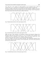
Fig. 15 shows the distributions of the near-wall hydrodynamic conditions, V
xa
, V
xf
, V
ya
, and
V

yf
, of the specimens. Only the distributions in the right-half of the apparatus are shown in
Mass Transfer Equation and Hydrodynamic Effects in Erosion-Corrosion

205
the figure. The average vertical velocity, V
ya
, was highest at the center of the specimen, since
the solution was injected vertically and toward the specimen. V
ya
showed a negative
pressure in the area outside of 5 mm, which was due to boundary-layer separation in the
area. The average horizontal velocity V
xa
was highest 5 mm from the center of the specimen,
which corresponded to the edge of the nozzle mouth, because the flow direction changed at
this location. The fluctuations in the vertical and horizontal velocities V
ya
and V
yf
were
highest in the area 10 mm from the center. As a result, the hydrodynamic parameters had
different distributions, and the region showing the maximum differed among these
parameters. Thus, we successfully measured the various hydrodynamic parameters in the
jet-in-slit corrosion testing apparatus.
-3
-2
-1
0
1

2
3
4
5
010203040
V
ya
V
yf
V
xf
V
xa
Distance from the center of the specimen / mm
Flow velocity / m·s
-1
0 2 4 6 8.

Fig. 15. The distributions of the near-wall hydrodynamic conditions, V
xa
, V
xf
, V
ya
and V
yf
, of
the specimens. Only the distributions in the right-half of the apparatus are shown in the figure.
To relate the hydrodynamic conditions to the corrosion damage, V
xa

, V
xf
and V
ya
were
selected as follows. Only positive pressure was used for V
ya
, because negative pressure in
the area outside the region 5 mm from the center was caused by boundary-layer separation
and was related to the fluctuations V
xf
and V
xf
. The vertical velocity fluctuation V
yf
was
similar to the horizontal velocity fluctuation V
xf
, so only V
xf
was used to predict the
corrosion damage.
4.3 Prediction of damage using hydrodynamic effects and mass transfer equation
The jet-in-slit testing apparatus shown in section 2.1 was used for the corrosion tests
performed under a flowing solution. Brass (58.3Cu-38.2Zn-3.10Pb-0.17Fe-0.23Sn) and
70CuNi (30.2Ni-Cu) were used as model materials for the corrosion tests. A 3% NaCl
solution and a 1 wt% CuCl
2
solution saturated with air were used as the corrosive test
solutions. The concentration of oxygen dissolved in the solutions was approximately 6.45

ppm. Cu
2+
in the 1 wt% CuCl
2
solution acted as the oxidizing agent to accelerate the
corrosion reaction. The test duration was 24 h in the 3% NaCl solution and 1 h in the 1 wt%
CuCl
2
solution.
Advanced Topics in Mass Transfer

206
Cross-sectional profiles of the brass and 70CuNi specimens after flow-induced localized
corrosion tests at a flow rate of 0.4 L· min
-1
are shown in Fig. 16. The thin line indicates the
profile before the test, which was determined as volume loss calculated from mass loss and
the density of a specimen coinciding to the volume loss calculated from the surface profile
before and after the test, as explained in section 2.2.
Brass
70CuNi
2 mm
40 μm
2 mm
10 μm
A
B
B
A
B

B

Fig. 16. Cross-sectional profiles of the brass (upper) and 70CuNi (lower) specimens after
flow-induced corrosion tests at a flow rate of 0.4 L min
-1
. The thin line is the profile before
the test.
Brass was significantly damaged in the central region of the specimen (region A) and in the
area approximately 2 mm from the center of the specimen (region B). The damage to the
periphery was relatively low. This result was obviously due to the hydrodynamic effects of
the corrosive solution. Similar to the brass specimen, the 70CuNi sample was significantly
damaged in the central area (regions A and B), compared with the damage to the periphery.
The damage in region B was deeper than that in region A for brass, but the damage in
region B was less than that in region A for 70CuNi. The result is likely due to differences in
the corrosion-product films that formed on the surface of each specimen under a flowing
solution, because the hydrodynamic conditions near the surface were very similar for the
two materials. The corrosion rate for both materials differed with the oxidizing agent
concentration. The flow-induced localized corrosion of copper alloys proceeded through
both the initiation step, which occurred following the mechanical destruction of the
corrosion-product film, and the propagation step, which occurred following the repeated
formation and breakaway of the products due to the local hydrodynamic effect (S. Nešić et
al., 1991; Bozzini et al., 2003). Since wet-polished specimens were tested in the present study,
most of the damage to the copper alloys occurred during the propagation step, which was
equal to the steady state. The porous corrosion-product film was detected by direct
observation of the specimen surface after the corrosion test.
The corrosion damage to the copper alloy in a 1 wt% CuCl
2
solution was much greater than
the damage that resulted from the 3% NaCl solution, as shown in Fig. 16. This result
indicated that the corrosion damage was mainly caused by the cathodic reaction. Thus, the

Mass Transfer Equation and Hydrodynamic Effects in Erosion-Corrosion

207
flow-induced localized corrosion of copper alloys mainly proceeds under cathodic control,
so that the rate-controlling step in corrosion is the transport of the oxidizing agent from the
bulk of the fluid to the metal surface. The corrosion rate should be proportional to the
diffusion rate of the oxidant. In the steady state, the corrosion rate, R
c
(m· s
-1
), can be given
by equation (4). Accordingly, the local damage d (μm) can be estimated using the testing
time t (h), as follows:
d = 3.6×10
9
Kc
b
t / ( 1/k
c
+ 1/k
d
) (11)
Assuming that the corrosion-product film that formed on the copper alloys was either
thicker than the concentration boundary layer or thinner but more dense, it had a structure
that resisted diffusion of the oxidizing agent. Therefore, the diffusion of the oxidizing agent
in the corrosion-product film was relatively low for the rate-controlling step, namely k
c
>>
k
d

. Thus equation (11) gives
d = 3.6×10
9
Kk
d
c
b
t (12)
The corrosion-product film that formed on the surface was in a steady state, and its
thickness and structure were determined by repeated formation and breakaway due to the
hydrodynamic effects. In this process, the condition of the film is determined by the
mechanical force acting on the film. When the velocity was high, the force acting on the film
was large, resulting in thinning of the film, so that the mass transfer coefficient in the
corrosion-product film became larger. Hence, the mass transfer coefficient in the corrosion-
product film k
d
(m· s
-1
) was assumed to be proportional to the velocities at the near-wall, as
follows:
k
d
= γ
xa
V
xa
+ γ
xf
V
xf

+ γ
ya
V
ya
(13)
where each γ is a material-specific constant that corresponds to the contributing ratio for
each hydrodynamic condition.
The damage depth profile for the copper alloys was calculated using equations (12) and (13)
as fitted to the experimental damage profile using a trial-and-error method. The calculated
and experimental profiles for brass and 70CuNi are shown in Figs. 17 and 18. The figures
show only the right-half of the damage profile for each specimen. The data used for brass
that was tested in a 3% NaCl solution were as follows: K = 3.6×10
-6
m
3
· mol
-1
(=
63.5/2/8.9×10
6
, where 63.5 g· mol
-1
is the molecular weight of copper, 2 is the number of
ion-exchanges in anodic and cathodic reactions, and 8.9×10
6
g· m
-3
is the density of copper),
c
b

= 0.20 mol· m
-3
, which corresponds to dissolved oxygen of 6.45 ppm, t=24 h, and the γ
values obtained by fitting to the measured data were: γ
xa
= 2.3×10
-7
, γ
xf
= 4.6×10
-5
and γ
ya
=
1.2×0
-6
, respectively.
The data used for 70CuNi that was tested in a 1 wt% CuCl
2
solution were as follows: K = 7.1
x 10
-6
m
3
· mol
-1
(=63.5/1/8.9×10
6
, where 63.5 g· mol
-1

is the molecular weight of copper, 1 is
the number of ion-exchanges in anodic and cathodic reactions, and 8.9×10
6
g· m
-3
is the
density of 70CuNi). c
b
= 74 mol· m
-3
, which corresponds to the Cu
+
concentration of the 1
wt% CuCl
2
solution, t = 1 h, and the γ values obtained for each material from fitting to the
measured data were: γ
xa
= 3.8×10
-6
, γ
xf
= 8.8×10
-6
, γ
ya
= 3.5×10
-6
, respectively. The calculated
profiles were consistent with both the experimental data and the areas of maximal damage

for both copper alloys—2 mm for brass and 1 mm for 70CuNi. Comparing the contributing
ratio (γ) to each hydrodynamic condition, the fluctuation in horizontal velocity, γ
xf
, was

Advanced Topics in Mass Transfer

208
Distance from the center of specimen / mm
Damage depth / μm
Brass
0
2
4
6
8
10
12
Calculated
Experimental
0 1 2 3 4 5 6 7 8

Fig. 17. The experimental and calculated damage depth profiles for brass tested in the 3%
NaCl solution for 24 h. The figures show only the right half of the specimen.

Distance from the center of specimen / mm
Damage depth / μm
70CuNi
0 1 2 3 4 5 6 7 8
0

20
40
60
80
100
Calculated
Experimental

Fig. 18. The experimental and calculated damage depth profiles for 70CuNi tested in the 1
wt% CuCl
2
solution for 1 h. The figures show only the right half of the specimen.
dominant in the corrosion damage of brass. On the other hand, average vertical velocity, γ
xa
,
also affected the corrosion damage of 70CuNi, in addition to the fluctuation of horizontal
velocity, γ
xf
. Thus, the hydrodynamic effect on the corrosion damage of copper alloys was
not attributed to a single parameter, such as flow velocity or Sherwood number, but instead
was related to multiple effects from both horizontal and vertical force and fluctuation. The
material-specific constant γ in equation (13) is related to the mechanical properties of the
corrosion-product films that formed on the surface of copper alloys. Consequently, these
properties are particularly important for the prediction of corrosion damage under a
flowing solution.
Mass Transfer Equation and Hydrodynamic Effects in Erosion-Corrosion

209
7. Conclusion
Erosion-corrosion tests were carried out using a jet-in-slit testing apparatus, and the

following results were obtained. The damage depth rate of Cu, BeCu and 70CuNi increased
with increasing flow velocity, and the breakaway velocity was clearly evident. The films
that formed on Cu and 70CuNi were significantly damaged by turbulence, such that the
hydrodynamic conditions of the flowing solution affected the breakaway property of the
corrosion-product film. Damage depth rate, calculated by the mass transfer equation, which
involved mass transfer in the concentration diffusion layer and in the corrosion-product
film, could to be fitted to the experimental damage rate. Thus, we confirmed that the mass
transfer equation can be applied to erosion-corrosion damage to copper and copper alloys.
The film condition remained nearly constant at a velocity lower than the breakaway
velocity, and the films that formed on BeCu, 70CuNi and 30CuNi were enhanced more than
two-fold compared with the film that formed on pure Cu, as evidenced by the analysis of
the mass transfer coefficient in the corrosion-product film. The corrosion-product film was
exponentially broken away at velocities greater than the breakaway velocity. The breakaway
property of the corrosion-product film differed among the materials, since the power of the
exponential equation was different for each material.
The relationship between the near-wall hydrodynamic effects on the material surface and
the corrosion damage of material under a flowing solution was investigated. The near-wall
hydrodynamic conditions on the surface of the test specimens were measured using
pressure gauges, and both the distribution of the near-wall velocity and the velocity
fluctuations were determined. Three types of hydrodynamic conditions were applied as
parameters that are related to the mass transfer coefficient in a corrosion-product film in the
equation used to predict corrosion damage. The damage profiles calculated from the
equation could be fitted to that obtained from the corrosion test using the three
hydrodynamic parameters. The determined material-specific constant agreed with the
mechanical resistance of the corrosion-product film to the hydrodynamic effects in a
corrosive liquid. Consequently, the mechanical properties of the corrosion-product films
that formed on the surface of the copper alloys are particularly important for the prediction
of corrosion damage under a flowing solution.
8. References
Bird R.B.; Stewart W.E. & Lightfoot E.N. (1960). Transport phenomena, John Wiliey & Sons,

INC., pp. 647, ISBN 0-471-07392-X, New York.
Bozzini B.; Ricotti M.E.; Boniardi M. & Mele C. (2003). Evaluation of erosion–corrosion in
multiphase flow via CFD and experimental analysis, Wear, Vol.255, No.1-6, 237-245,
ISSN 0043-1648.
Chexal B.; Horowitz J.; Jones R.; Dooley B.; Wood C.; Bouchacourt M.; Remy F.; Nordmann
F. & Paul P.St. (1996). Flow-Accelerated Corrosion in Power Plants, EPRI Distribution
Center, ISBN TR-106611, Pleasant Hill, CA.
Ferng Y.M.; Ma Y.P. & Chung N.M. (2000). Application of local flow models in predicting
distributions of erosion-corrosion locations, Corrosion, Vol.56, No.2, 116-126, ISSN
0010-9312.
Keating A. & Nešić S. (2001). Numerical prediction of erosion-corrosion in bends, Corrosion,
Vol.57, No.7, 621-633, ISSN 0010-9312.
Advanced Topics in Mass Transfer

210
Mahato B.K.; Cha C.Y. & Shemilt L.W. (1980). Unsteady state mass transfer coefficients
controlling steel pipe corrosion under isothermal flow conditions, Corrosion Science,
Vol.20, No.3, 421-441, ISSN 0010-938X.
Matsumura M.; Oka Y.; Okumoto S. & Furuya H. (1985). Laboratory Corrosion Tests and
Standards STP 866, ASTM, pp.358-372, ISBN 0-8031-0443-X, Philadelphia.
Matsumura M.; Noishiki K. & Sakamoto A. (1988). Jet-in-slit test for reproducing flow-
induced localized corrosion on copper alloys, Corrosion, Vol.54, 79-88, ISSN 0010-
9312.
Murakami, M.; Sugita K.; Yabuki A & Matsumura M. (2003). Mechanism of so-called
erosion-corrosion and flow velocity difference corrosion of pure copper, Corrosion
Engineering (Zairyo-to-Kankyo), Vol.52, No. 3, 155-159, ISSN 0917-0480.
Nešić S. & Postlethwaite J. (1991). Hydrodynamics of disturbed flow and erosion-corrosion.
Part I-Single-phase flow study, The Canadian Journal of Chemical Engineering,
Vol.69, No. 3, 698-703, ISSN 00084034.
Postlethwaite J.; Nešić S.; Adamopoulos G. & Bergstrom D.J. (1993). Predictive models for

erosion-corrosion under disturbed flow conditions, Corrosion Science, Vol.35, No.1-
4, 627-633, ISSN 0010-938X. Poulson B. (1983). Electrochemical measurements in
flowing solutions, Corrosion Science, Vol.23, No.4, 391-430, ISSN 0010-938X.
Poulson B. (1993). Advances in understanding hydrodynamic effects on corrosion, Corrosion
Science, Vol.35, No.1-4, 655-665, ISSN 0010-938X.
Poulson B. (1999). Complexities in predicting erosion corrosion, Wear, Vol.233-235, 497-504,
ISSN 0043-1648.
Sydberger T. & Lotz U. (1982). Relation Between Mass Transfer and Corrosion in a
Turbulent Pipe Flow, J. Electrochem. Soc., Vol.129, No.2, 276-283, ISSN 0013-4651.
Syrett B.C. (1976). Erosion-corrosion of copper-nickel alloys in seawater and other aqueous
environments – a Literaturee review, Corrosion, Vol.32, 242-252, ISSN 0010-9312.
Wharton J.A. & Wood R.J.K. (2004). Influence of flow conditions on the corrosion of AISI
304L stainless steel, Wear, Vol.256, No.5, 525-536, ISSN 0043-1648.
11
Hydrodynamics and Mass Transfer in
Heterogeneous Systems
Radmila Garić-Grulovic
1
, Nevenka Bošković-Vragolović
2
,
Željko Grbavčić
2
and Rada Pjanović
2

1
Institute for Chemistry, Technology and Metallurgy, University of Belgrade
2
Faculty of Technology and Metallurgy, University of Belgrade

Serbia
1. Introduction
Research of transport phenomena in liquid – particles systems, in past years, had a more
theoretical then practical importance (Coudrec, 1985; Lee et al., 1997; Schmidt et al., 1999).
For industrial use, especially with fast development of bio and water cleaning processes,
better knowing of these systems become more important. An industrial application of these
systems requires determination of transfer characteristics, especially mass transfer.
Frequently mass transfer is the rate determining step in the whole process. However, in the
real systems, it is not always easy to differentiate the limitation due to the mass transfers
from that due to the hydrodynamic.
Mass transfer in liquid-solid packed and fluidized beds has been widely investigated in
terms of particle–fluid mass transfer by dissolution, by electrochemical and by ion-exchange
methods (Damronglerd et al. 1975; Koloini et al. 1976; Dwivedi & Upadhyay, 1977; Chun &
Couderc, 1980; Kumar & Upadhyay, 1981; Rahman & Streat, 1981; Yutani et al. 1987). Some
of the results of mass transfer in packed and fluidized beds have been obtained as the
transfer between an immersed surface and the liquid (Riba et al. 1979; Bošković et al. 1994;
Bošković-Vragolović, et al., 1996&2005). Liquid fluidization of particulate solids has a
history which predates the now more commonly applied gas fluidization. The broad range
of operations to which liquid fluidization has found applications are: classification of
particles by size and density, a special case being sink-and-float separation by density;
backwashing of granular filters and washing of soils; crystal growth; leaching and washing;
adsorption and ion exchange; electrolysis with both inert and electrically conducting
fluidized particles; liquid-fluidized bed heat exchangers and thermal energy storage; and
bioreactors. Fluidized-bed bioreactors, which have received much attention during the past
thirty years, are usually characterized by the catalytic use of enzymes or microbial cells that
are immobilized by attachment, entrapment, encapsulation or self-aggregation. The most
common application of such bioreactors is probably in wastewater treatment and, as in the
case of the other operations mentioned above, liquid fluidization must in each case be
weighed against competing schemes for achieving the same objective before it is adopted
commercially (Epstein, 2003). In contrast to fluidized beds data, there are no published data

on mass transfer in vertical and horizontal hydrotransport of particles.
Advanced Topics in Mass Transfer

212
Liquid–solid packed and fluidized beds have usually been investigated separately (Kumar &
Upadhyay, 1981; Yutani et al. 1987; Comiti & Renaud, 1991; Schmidt et al., 1999), but many
authors have noticed the similarity between the two systems (Dwivedi & Upadhyay, 1977).
2. Background of heterogeneous systems
There are a number of different types of systems designed for fluid-solid heterogeneous
operations. Two-phase flow systems of fluid (gas or liquid) and particles, the way of
realizing contact between the phases, namely how the introduction of fluid in the bed of
particles can be (Fig. 1):
systems with a fixed bed of particles;
- packed bed (a),
systems with a moving bed of particles;
- Fluidized bed (b),
- spouted bed and spout-fluid beds (c),
- spouted bed and spout-fluid beds with draft tube (d),
- vertical two-phase flow systems (fluid-particle), i.e. transport systems (e).
Packed beds are an essential part of chemical engineering equipment. A packed bed is a
column filled with a support material, in which one or more fluids flow (Fig. 1, a). In
chemical processing, a packed bed is a hollow tube, pipe, or other vessel that is filled with a
packing material. The packing can be randomly filled with small objects like Raschig rings
or else it can be a specifically designed structured packing. Differently shaped packing
materials have different surface areas and void space between the packing. Both of these
factors affect packing performance. The purpose of a packed bed is typically to improve
contact between two phases in a chemical or similar process. Packed beds are widely used in
industry to contact two or more fluid phases at relatively low pressure drops. For process
design purposes, it is essential that pressure drop be estimated for its proper operation.
They are readily used in industry for catalytic reactions, combustion, gas absorption,

distillation, drying, and separation processes.
A fluidized bed is a packed bed through which fluid flows at such a high velocity that the
bed is loosened and the particle-fluid mixture behaves as though it is a fluid (Fig. 1, b). Thus,
when a bed of particles is fluidized, the entire bed can be transported like a fluid, if desired.
Both gas and liquid flows can be used to fluidize a bed of particles. In fluidized beds, the
contact of the solid particles with the fluidization medium (a gas or a liquid) is greatly
enhanced when compared to packed beds. The most common reason for fluidizing a bed is
to obtain vigorous agitation of the solids in contact with the fluid, leading to excellent
contact of the solid and the fluid and the solid and the wall. Fluidized beds are widely used
in industry for mixing solid particles with gases or liquids. In most industrial applications, a
fluidized bed consists of a vertically-oriented column filled with granular material, and a
fluid (gas or liquid) is flow upward through a distributor at the bottom of the bed.
Fluidized bed technology has become a common method to increase heat and mass transfer
in physical and chemical operations. Although a great amount of studies have been
performed to characterize the physical properties of these systems, only a few satisfying
models have been derived. This is especially true for liquid-solid fluidized beds, which
usually play a minor role in practical applications. Furthermore, studies dealing with gas-
solid or gas-liquid-solid fluidized beds may not be applied to liquid-solid fluidized beds,
because of the very different physical behaviour of these systems (Schmidt et al., 1999).
Hydrodynamics and Mass Transfer in Heterogeneous Systems

213

(a) (b) (c) (d) (e)
Fig. 1. Schematic diagram of heterogeneous systems:
a. Packed bed,
b. Fluidized bed,
c. Spout/Spout-fluid bed,
d. Spout/Spout-fluid bed with draft tube,
e. Vertical two-phase flow system (transport system).

A spouted bed can be formed in a vertical column where the fluid jet blows vertically upwards
along the centre line of the centre line of the column thus forming a spout in which there is a
fast moving fluid and entrained particle (Fig. 1, c). The remainder of the bed, the annulus
between the spout and the column wall, is densely packed with particles moving slowly
downwards and radially inwards. Fluid percolates through these particles from the spout.
The spouted bed technique, originally developed by Mathur & Gishler, 1955, has been
successfully applied to a variety of diffusional, thermal, mechanical and other processes.
Various modifications of the classical spouted bed have been proposed to improve its
operability and provide better agreement between bed characteristics and process
requirements. By introducing external annular fluid flow through the annulus bottom,
spout-fluid bed can be formed (Nagarkatti & Chatterjee, 1974; Vuković et al., 1984; Sutanto
et al., 1985). The draft tube in these systems is essentially a pneumatic or hydraulic riser which
is relatively short even in the industrial scale units.
The addition, a draft tube in a spout and spout-fluid bed changes some of basic their
characteristics (Fig. 1, d). The most important of these are:
- there is no bed height limitation imposed by a maximum spout and spout-fluid bed
height.
- the minimum spout and spout-fluid (or circulating) velocity is lower in a bed with a
draft tube.
- the draft tube forces all of the particles to travel through the entire annulus section
surrounding the draft tube before re-entering the spout in the entry section thereby
narrowing the particle residence time distribution in the annulus.