Advances in Sound Localization Part 4 docx
Bạn đang xem bản rút gọn của tài liệu. Xem và tải ngay bản đầy đủ của tài liệu tại đây (2.18 MB, 40 trang )
7
Sound Source Localization Method
Using Region Selection
Yong-Eun Kim
1
, Dong-Hyun Su
2
, Chang-Ha Jeon
2
,
Jae-Kyung Lee
2
,
Kyung-Ju Cho
3
and Jin-Gyun Chung
2
1
Korea Automotive Technology Institute in Chonan,
2
Chonbuk National University in Jeonju,
3
Korea Association Aids to Navigation in Seoul,
Korea
1. Introduction
There are many applications that would be aided by the determination of the physical
position and orientation of users. Some of the applications include service robots, video
conference, intelligent living environments, security systems and speech separation for
hands-free communication devices (Coen, 1998; Wax & Kailath, 1983; Mungamuru &
Aarabi, 2004; Sasaki et al., 2006; Lv & Zhang 2008). As an example, without the information
on the spatial location of users in a given environment, it would not be possible for a service
robot to react naturally to the needs of the user.
To localize a user, sound source localization techniques are widely used (Nakadai et al.,
2000; Brandstein & Ward, 2001; Cheng & Wakefield, 2001; Sasaki et al., 2006). Sound
localization is the process of determining the spatial location of a sound source based on
multiple observations of the received sound signals. Current sound localization techniques
are generally based upon the idea of computing the time difference of arrival (TDOA)
information with microphone arrays (Knnapp & Cater, 1976; Brandstein & Silverman, 1997).
An efficient method to obtain TDOA information between two signals is to compute the
cross-correlation of the two signals. The computed correlation values give the point at which
the two signals from separate microphones are at their maximum correlation. When only
two isotropic (i.e., not directional as in the mammalian ear) microphones are used, the
system experiences front-back confusion effect: the system has difficulty in determining
whether the sound is originating from in front of or behind the system. A simple and
efficient method to overcome this problem is to incorporate more microphones (Huang et
al., 1999).
Various weighting functions or pre-filters such as Roth, SCOT, PHAT, Eckart filter and HT
can be used to increase the performance of time difference estimation (Knnapp & Cater,
1976). However, the performance improvement is achieved with the penalty of large power
consumption and hardware overhead, which may not be suitable for the implementation of
portable systems such as service robots.
In this chapter, we propose an efficient sound source localization method under the
assumption that three isotropic microphones are used to avoid the front-back confusion
Advances in Sound Localization
108
effect. By the proposed approach, the region from 0° to 180° is divided into three regions
and only one of the three regions is selected for the sound source localization. Thus
considerable amount of computation time and hardware cost can be reduced. In addition,
the estimation accuracy is improved due to the proper choice of the selected region.
2. Sound localization using TDOA
If a signal emanated from a remote sound source is monitored at two spatially separated
sensors in the presence of noise, the two monitored signals can be mathematically modeled as
111
21 2
() () (),
() ( ) (),
xt st nt
xt stD nt
=+
=α − +
(1)
where
α and D denote the relative attenuation and the time delay of ()
2
tx with respect to
(),
1
tx respectively. It is assumed that signal ()
1
ts and noise ()
i
ntare uncorrelated and jointly
stationary random processes. A common method to determine the time delay D is to
compute the cross correlation
12
12
() [ () ( )]
xx
RExtxt
τ
=−τ, (2)
where
E denotes expectation operator. The time argument at which
12
()
xx
R τ achieves a
maximum is the desired delay estimate.
Fig. 1. Sound source localization using two microphones
Fig. 1 shows the sound localization test environments using two microphones. We assume
that the sound waves arrive in parallel to each microphone as shown in Fig. 1. Then, the
time delay
D can be expressed as
cos
mic
sound sound
l
d
D
vv
==
φ
, (4)
where
sound
v denotes the sound velocity of 343m/s. Thus, the angle of the sound source is
computed as
11
cos cos
sound
mic mic
Dv
d
ll
−−
= =
φ
. (5)
If the sound wave is sampled at the rate of
s
f
, and the sampled signal is delayed
by
d
n samples, the distance d can be computed as
Sound Source Localization Method Using Region Selection
109
sound d
s
vn
d
f
=
. (6)
In Fig. 1, since
d is a side of a right-angled triangle, we have
mic
dl< . (7)
Thus, when
mic
dl= in (6), the number of maximum delayed samples
,maxd
n is obtained as
,max
smic
d
sound
fl
n
v
= . (8)
3. Proposed sound source localization method
3.1 Region selection for sound localization
The desired angle in (5) is obtained using the inverse cosine function. Fig. 2 shows the
inverse cosine graph as a function of
d. Since the inverse cosine function is nonlinear, Δd
(estimation error in d) has different effect on the estimated angle depending on the sound
source location. Fig. 3 shows the estimation error (in degree) of sound source location as a
function of Δ
d. As can be seen from Fig. 3, Δd has smaller effect for the sources located from
60° to 120°. As an example, when the source is located at 90° with the estimation error Δ
d =
0.01, the mapped angle is 89.427°. However, if the source is located at 0° with the estimation
error Δ
d = 0.01, the mapped angle is 8.11°. Thus, for the same estimation error Δd, the effect
for the source located at 0° is 14 times larger than that of the source at 90°. To efficiently
implement the inverse cosine function, we consider the region from 60° to 120° as
approximately linear as shown in Fig. 2.
Fig. 2. Inverse cosine graph as a function of
d
Advances in Sound Localization
110
Fig. 3. Estimation error of sound source location as a function of Δ
d
Fig. 4 shows the front-back confusion effect: the system has difficulty in determining
whether the sound is originating from in front of (sound source A) or behind (sound source
B) the system. A simple and efficient method to overcome this problem is to incorporate
more microphones. In Fig. 5, three microphones are used to avoid the front-back confusion
effect, where L, R and B mean the microphones located at the left, right and back sides,
respectively. In this chapter, to apply the cross-correlation operation in (2), for each arrow
between the microphones in Fig. 5, the signal received at the tail part and the head part are
designated as
1
()xtand
2
(),xt respectively.
In conventional approaches, correlation functions are calculated between each microphone
pair and mapped to angles as shown in Fig. 6-(a), (b) and (c). Notice that, due to the front-
back confusion effect, each microphone pair provides two equivalent maximum values. Fig.
6-(d) is obtained by adding the three curves. In Fig. 6-(d), the angle corresponding to the
maximum magnitude is the desired sound source location.
Fig. 4. Front-back confusion effect
Sound Source Localization Method Using Region Selection
111
Fig. 5. Sound source localization using three microphones
(a)
(b)
(c)
(d)
Fig. 6. Angles obtained from microphone pairs: (a) L-R, (b) B-L, (c) R-B, and (d) (L-R)+
(B-L)+(R-B)
Advances in Sound Localization
112
Source location(angle) Proper microphone pair
60°~120°, 240°~300°
R-L
120°~180°, 300°~360°
B-R
180°~240°, 0°~60°
L-B
Table 1. Selection of proper microphone pair for six different source locations.
Due to the nonlinear characteristic of the inverse cosine function, the accuracy of each
estimation result is different depending on the source location. Notice that in Fig. 5,
wherever the source is located, exactly one microphone pair has the sound source within its
approximately linear region (60°~120° or 240°~300° for the microphone pair). As an
example, if a sound source is located at 30° in Fig. 5, the location is within the approximately
linear region for L-B pair. Table 1 summarizes the choice of proper microphone pairs for six
different source locations.
The proper selection of microphone pairs can be achieved by comparing the time index
max
τ
values (or, the number of shifted samples) in (2) at which the maximum correlation values
are obtained. Fig. 7 shows the comparison of the correlation values obtained from three
microphone pairs when the source is located at 90°. For the smallest estimation error, we
select the microphone pair whose
max
τ value is closest to 0. Notice that the correlation curve
in the center (by the microphone pair R-L) has the
max
τ value which is closest to 0.
In fact, for the smallest estimation error, we just need to select the correlation curve in the
center. As an example, assume that a sound source is located at 90° in Fig. 5. Then, for the
microphone pair R-L, the two signals arrived at the microphones R and L have little
difference in their arrival times since the distances from the source to each microphone are
almost the same. Thus, the cross correlation has its maximum around
0.τ= However, for L-
B pair, the microphone L is closer to the source than the microphone B. Since the received
signals at microphones B and L are designated as
1
()xtand
2
(),xt respectively, the cross
Fig. 7. Comparison of the correlation values obtained from three microphone pairs for the
source located at 90°
Sound Source Localization Method Using Region Selection
113
correlation in (2) gets its maximum when
2
()xt is shifted to the right ( 0
τ
> ). The opposite is
true for the microphone pair B-R as can be seen from Fig. 7.
Table 2 shows that proper microphone pairs can be simply selected by comparing maximum
correlation positions (or,
max
τ values from each microphone pair).
Maximum correlation positions Proper Mic. Front / Back
max
τ (BR)≤
max
τ (RL) ≤
max
τ (LB)
R-L Front
max
τ (BR)≤
max
τ (LB) ≤
max
τ (RL)
L-B Front
max
τ (RL)≤
max
τ (BR) ≤
max
τ (LB)
B-R Front
max
τ (LB)≤
max
τ (RL) ≤
max
τ (BR)
R-L Back
max
τ (RL)≤
max
τ (LB) ≤
max
τ (BR)
L-B Back
max
τ (LB)≤
max
τ (BR) ≤
max
τ (RL)
B-R Back
Table 2. Selecetion of proper microphone pair
If the sampled signals of
()
1
tx and ()
2
tx are denoted by two vectors X
1
and X
2
, the length of
the cross-correlated signal R
X1X2
is determined as
n(R
X1X2
) = n(X
1
) + n(X
2
) – 1, (9)
where
n(X) means the length of vector X. In other words, to obtain the cross-correlation
result, vector shift and inner product operations need to be performed by n(R
X1X2
) times.
It is interesting to notice that, once the distance between the microphones and the sampling
rate are determined, the maximum time delay between two received signals is bounded by
,maxd
n in (8). Thus, instead of performing vector shift and inner product operations by
n(R
X1X2
) times as in the conventional approaches, it is sufficient to perform the operations by
only
,maxd
n times. Specifically, we perform the correlation operation from
,maxd
nn=− /2 to
,maxd
nn= /2 (for sampled signals, ,/
s
f
nτ= integer n). In the simulation shown in Fig. 7,
n(X
1
) = n(X
2
) = 256 and
,max
.64
d
n = Thus, the number of operations for cross-correlation is
reduced from 511 to 65 by the proposed method, which means the computation time for
cross-correlation can be reduced by 87%.
3.2 Simplification of angle mapping using linear equation
Conventional angle mapping circuits require a look-up table for inverse cosine function.
Also, an interpolation circuit is needed to obtain a better resolution with reduced look-up
table. However, since the proposed region selection approach uses only the approximately
linear part of the inverse cosine function, the use of look-up table and interpolation circuit
can be avoided. Instead, the approximately linear region is approximated by the following
equation:
y
ax b
=
+ , (10)
Advances in Sound Localization
114
where
60
,
(cos /3 cos2 /3)
60cos2 /3
120 .
(cos /3 cos2 /3)
mic
a
l
b
−
=
π− π ×
π
=+
π− π
(11)
When the distance between the two microphones is given, the coefficients a and b in (10) can
be pre-calculated. Thus, angle mapping can be performed using only one multiplication and
one addition for a given value of d.
Fig. 8 shows the block diagrams of the conventional sound source localization systems and
the proposed system.
(a)
(b)
Fig. 8. Block diagrams of conventional and proposed methods: (a) conventional method, and
(b) proposed method.
4. Simulation results
Fig. 9 shows the sound source localization system test environments. The distance between
the microphones is 18.5cm. The sound signals received using three microphones are
sampled at 16 KHz and the sampled signals are sent to the sound localization system
implemented using Altera stratix II FPGA. Then, the estimation result is transmitted to a
host PC through two FlexRay communication systems. The test results are shown in Table 3.
Notice that the average error of the proposed method is only 31% of that of the conventional
method. To further reduce the estimation error, we need to increase the sampling rate and
the distance between the microphones.
Sound Source Localization Method Using Region Selection
115
Fig. 9. Sound localization system test environments
Distance 0° 30° 60° 90°
1m 0° 27° 56° 88°
2m 0° 27° 59° 85°
3m 0° 27° 59° 88°
4m 2.5° 34° 57° 95°
5m 4.1° 37° 67° 82°
Maximum absolute error 4.1° 7° 7° 8°
average error 1.32° 4° 3.2° 4.4°
(a)
Distance 0° 30° 60° 90°
1m 0° 32.7° 60° 87.2°
2m 0° 32° 59° 85°
3m 0° 32.7° 60° 87.2°
4m 1 28° 62° 86°
5m 2 33° 61° 92°
Maximum absolute error 2° 3° 2° 4°
average error 0.6° 2.48° 0.8° 3.32°
(b)
Table 3. Simulation results: (a) conventional method, and (b) proposed method
5. Conclusion
Compared with conventional sound source localization methods, proposed method
achieves more accurate estimation results with reduced hardware overhead due to the new
region selection approach. By the proposed approach, the region from 0° to 180° is divided
into three regions and only one of the three regions is selected such that the selected region
corresponds to the linear part of the inverse cosine function. By the proposed approach, the
Advances in Sound Localization
116
computation time for cross correlation is reduced by 87%, compared with the conventional
approach. By simulations, it is shown that the estimation error by the proposed method is
only 31% of that of the conventional approach.
The proposed sound source localization system can be applied to the implementation of
portable service robot systems since the proposed system requires small area and low power
consumption compared with conventional methods. The proposed method can be combined
with generalized correlation method with some modifications.
6. Acknowledgment
This research was financially supported by the Ministry of Education, Science Technology
(MEST) and National Research Foundation of Korea (NRF) through the Human Resource
Training Project for Regional Innovation.
7. References
Brandstein M. S. & Silverman H. (1997). A practical methodology for speech source
localization with microphone arrays. Comput. Speech Lang., Vo.11, No.2, pp. 91-126,
ISSN 0885-2308
Brandstein M. & Ward D. B. (2001). Robust Microphone Arrays: Signal Processing Techniques
and Applications, New York: Springer, ISBN 978-3540419532
Cheng I. & Wakefield G. H. (2001). Introduction to head-related transfer functions (HRTFs):
representations of HRTFs in time, frequency, and space. J. Audio Eng. Soc., Vol. 49,
No.4, (April, 2001), pp. 231-248, ISSN 1549-4950
Coen M. (1998). Design principles for intelligent environments, Proceedings of the 15th
National Conference on Artificial Intelligence, pp. 547-554
Huang J.; Supaongprapa T.; Terakura I.; Wang F.; Ohnishi N. & Sugie N. (1999) A model-
based sound localization system and its application to robot navigation. Robot.
Auton. Syst., Vol.27, No.4, (June,1999), pp. 199-209, ISSN 0921-8890
Knnapp C. H. & Cater G. C. (1976). The generalized correlation method for estimation of
time delay. IEEE Trans. Acoust. Speech Signal Process., Vol.24, No.4, (August 1976),
pp.320-327, ISSN 0096-3518
Lv X. & Zhang M. (2008). Sound source localization based on robot hearing and vision,
Proceedings of ICCSIT 2008 International Conference of Computer Science and
Information Technology, pp. 942-946, ISBN 978-0-7695-3308-7, Singapore, August 29-
September 2 2008
Mungamuru, B. & Aarabi, P. (2004). Enhanced sound localization. IEEE Trans. Syst. Man
Cybern. Part B- Cybern., Vol.34, No.3, (June, 2004), pp. 1526-1540, ISSN 1083-4419
Nakadai K.; Lourens T.; Okuno H. G. & Kitano H. (2000). Active audition for humanoid,
Proceedings of the 17th National Conference on Artificial Intelligence and 12th Conference
on Innovative Applications of Artificial Intelligence, pp. 832-839
Sasaki Y.; Kagami S. & Mizoguchi H. (2006). Multiple sound source mapping for a mobile
robot by self-motion triangulation, Proceedings of the 2006 IEEE/RSJ International
Conference on Intelligent Robots and Systems, pp. 380-385, ISBN 1-4244-0250-X,
Beijing, China, October, 2006
Wax M. & Kailath T. (1983). Optimum localization of multiple sources by passive arrays.
IEEE Trans. Acoust. Speech Signal Process., Vol.31, No.6, (October,1983). pp. 1210-
1217, ISSN 0096-3518
8
Robust Audio Localization for
Mobile Robots in Industrial Environments
Manuel Manzanares, Yolanda Bolea and Antoni Grau
Technical University of Catalonia, UPC, Barcelona
Spain
1. Introduction
For autonomous navigation in workspace, a mobile robot has to be able to know its position
in this space in a precise way that means that the robot must be able to self-localize to move
and perform successfully the different entrusted tasks. At present, one of the most used
systems in open spaces is the GPS navigation system; however, in indoor spaces (factories,
buildings, hospitals, warehouses…) GPS signals are not operative because their intensity is
too weak. The absence of GPS navigation systems in these environments has stimulated the
development of new local positioning systems with their particular problems. Such systems
have required in many cases the installation of beacons that operate like satellites (similar to
GPS), the use of landmarks or even the use of other auxiliary systems to determine the
robot’s position.
The problem of mobile robot localization is a part of a more global problem because in
autonomous navigation when a robot is exploring an unknown environment, it usually
needs to obtain some important information: a map of the environment and the robot’s
location in the map. Since mapping and localization are related to each other, these two
problems are usually considered as a single problem called simultaneous localization and
mapping (SLAM). The problem of Simultaneous Localization and Map Building is a
significant open problem in mobile robotics which is difficult because of the following
paradox: to localize itself the robot needs the map of the environment, and, for building a
map the robot location must be known precisely.
Mobile robots use different kinds of sensors to determine their position: for instance it is very
common the use of odometric or inertial sensors, however it is remarkable to consider that in
wheel slippage, sensor drifts a noise causing error accumulation, thus leading to erroneous
estimates. Another kind of external sensors used in robotics in order to solve localization are
for instance CCD cameras, infrared sensor, ultra sonic sensor, mechanical wave and laser.
Other sensors recently applied are the instruments sensible to the magnetic field known as the
electronic compass (Navarro & Benet, 2009). Mobile robotics are interested on those able to
measure the Earths magnetic field and express it through an electrical signal. One type of
electronic compass is based on magneto-resistive transducers, whose electrical resistance
varies with the changes on the applied magnetic field. This type of sensors presents
sensitivities below 0.1 milligauss, with response times below 1 sec, allowing its reliable use in
vehicles moving at high speeds (Caruso, 2000). In SLAM some applications with electronic
compass have been developed working simultaneously with other sensors such as artificial
vision (Kim et al., 2006) and ultrasonic sensors (Kim et al., 2007).
Advances in Sound Localization
118
In mobile robotics, due to the use of different sensors at the same time to provide
localization information the problem of data fusion rises and many algorithms have been
implemented. Multisensor fusion algorithms can be broadly classified as follows: estimation
methods, classification methods, inference methods, and artificial intelligence methods (Luo
et al., 2002); in the latter are remarkable neural networks, fuzzy and genetic algorithms
(Begum et al., 2006); (Brunskill & Roy, 2005). Related with the provided sensors information
processing in SLAM context, many works can be found, for instance in (Di Marco et al.,
2000), where estimation of the position of the robot and the selected landmarks are derived
in terms of uncertainty regions, under the hypothesis that the errors affecting all sensor
measurements are unknown but bounded, or in (Begum et al., 2006) where an algorithm
processes sensor data incrementally and therefore, has the capability to work online.
Therefore a comprehensive collection of researches have been reported on SLAM, most of
which stem from the pioneer work of (Smith et al. 1990). This early work provides a Kalman
Filter (KF) based statistical framework for solving SLAM. The KF based SLAM algorithms
require feature extraction and identification from sensor data, for estimating the pose and
the parameters. In the situation that the system noise and measurement obey a Gaussian
amplitude distribution, KF uses the state recursive equation that is with the noise estimates
the optimal attitude of mobile robots. But there would be generated errors of localization, if
the noise does not obey the distribution. KF is also able to the merge low graded multisensor
data models. Particle filter is the next probabilistic technique that has earned popularity in
SLAM literature. The hybrid SLAM algorithm proposed in (Thrun, 2001) uses particle filter
for posterior estimation over a robot’s poses and is capable to map large cyclic
environments. Another method of fusion broadly used is Extended Kalman Filter (EKF); the
EKF can be used where the model is nonlinear, but it can be suitably linearized around a
stable operating point.
Several systems have been researched to overcome the localization limitation. For example,
the Cricket Indoor Location (Priyantha, 2000) which relies on active beacons placed in the
environment. These beacons transmit simultaneously two signals (a RF and an ultrasound
wave). Passive listeners mounted, for example, on mobile robots can, by knowing the
difference in propagation speed of the RF and ultrasound signals, estimate their own
position in the environment. GSM and WLAN technologies can also be used for localization.
Using triangulation methods and measuring several signal parameters such as the signal’s
angle and time of arrival, it becomes possible to estimate the position of a mobile
transmitter/receiver in the environment (Sayed et al., 2005). In (Christo et al., 2009), a
specific architecture is suggested for the use of multiples iGPS Web Services for mobile
robots localization.
Most of the mobile robot’s localization systems are based on robot vision, and robot vision is
also a hot spot in the research of robotics. Camera which is the most popular visual sensor is
widely used for the localization of mobile robots just now. However some difficulties occur
because of the limitation of camera’s visual field and the dependence on light condition. If
the target is not in the visual field of camera or the lighting condition is poor, the visual
localization system of the mobile robot cannot work effectively. Nowadays, the role of
acoustic perception in autonomous robots, intelligent buildings and industrial environments
is increasingly important and in the literature there are different works (Yang et al., 2007);
(Mumolo et al., 2003); (Csyzewski, 2003).
Comparing to the study on visual perception, the study on auditory is still in its infancy
stage. The human auditory system is a complex and organic information processing system,
Robust Audio Localization for Mobile Robots in Industrial Environments
119
it can feel the intensity of sound and space orientation information. Compared with vision,
audition has several unique properties. Audition is omni-directional. The sound waves have
strong diffraction ability; audition also is less affected by obstacles. Therefore, the audio
ability possessed by robot can make up the restrictions of other sensors such as limited view
or the non-translucent obstacles. Nevertheless, audio signal processing presents some
particular problems such as the effect of reverberations and noise signals, complex
boundary conditions and near-field effect, among others, and therefore the use of audio
sensors together with other sensors is common to determine the position and also for
autonomous navigation of a mobile robot, leading to a problem of data fusion. There are
many applications that would be aided by the determination of the physical position and
orientation of users. As an example, without the information on the spatial location of users
in a given environment, it would not be possible for a service robot to react naturally to the
needs of the user. To localize a user, sound source localization techniques are widely used.
Such techniques can also help a robot to self-localize in its working area. Therefore, the
sound source localization (one or more sources) has been studied by many researchers (Ying
& Runze, 2007); (Sasaki et al., 2006); (Kim et al., 2009). Sound localization can be defined as
the process of determining the spatial location of a sound source based on multiple
observations of the received sound signals. Current sound localization techniques are
generally based upon the idea of computing the time difference of arrival (TDOA)
information with microphone arrays (Brandstein & Silverman, 1997); (Knapp & Carter,
1976), or interaural time difference (ITD) (Nakashima & Mukai, 2005). The ITD is the
difference in the arrival time of a sound source between two ears, a representative
application can be found in (Kim & Choi, 2009) with a binaural sound localization system
using sparse coding based ITD (SITD) and self-organizing map (SOM). The sparse coding is
used for decomposing given sounds into three components: time, frequency and magnitude,
and the azimuth angle are estimated through the SOM. Other works in this field use
structured sound sources (Yi & Chu-na, 2010) or the processing of different audio features
(Rodemann et al., 2009), among other techniques.
The works that authors present in this Chapter are developed with audio signals generated
with electric machines that will be used to mobile robots localization in industrial
environments. A common problem encountered in industrial environments is that the
electric machine sounds are often corrupted by non-stationary and non-Gaussian
interferences such as speech signals, environmental noise, background noise, etc.
Consequently, pure machine sounds may be difficult to identify using conventional
frequency domain analysis techniques as Fourier transform (Mori et al., 1996), and statistical
techniques such as Independent Component Analysis (ICA) (Roberts & Everson, 2001).
The wavelet transform has attracted increasing attention in recent years for its ability in
signal features extraction (Bolea et al., 2003); (Mallat & Zhang, 1993), and noise elimination
(Donoho, 1999). While in many mechanical dynamic signals, such as the acoustical signals of
an engine, Donoho’s method seems rather ineffective, the reason for their inefficiency is that
the feature of the mechanical signals is not considered. Therefore, when the idea of
Donoho’s method and the sound feature are combined, and a de-noising method based on
Morlet wavelet is added, this methodology becomes very effective when applied to an
engine sound detection (Lin, 2001). In (Grau et al., 2007), the authors propose a new
approach in order to identify different industrial machine sounds, which can be affected by
non-stationary noise sources.
Advances in Sound Localization
120
It is also important to consider that non-speech audio signals have the property of non-
stationary signals in the same way that many real signals encountered in speech processing,
image processing, ECG analysis, communications, control and seismology. To represent the
behaviour of a stationary process is common the use of models (AR, ARX, ARMA, ARMAX,
OE, etc.) obtained from the experimental identification (Ljung, 1987). The coefficient
estimation can be done with different criteria: LSE, MLE, among others. But in the case of
non-stationary signals the classical identification theory and its results are not suitable.
Many authors have proposed different approaches to modelling this kind of non-stationary
signals, that can be classified: i) assuming that a non stationary process is locally stationary
in a finite time interval so that various recursive estimation techniques (RLS, PLR, RIV, etc.)
can be applied (Ljung, 1987); ii) a state space modelling and a Kalman filtering; iii)
expanding each time-varying parameter coefficients onto a set of basis sequences
(Charbonnier et al., 1987); and iv) nonparametric approaches for non-stationary spectrum
estimation such a local evolving spectrum, STFT and WVD are also developed to
characterize non-stationary signals (Kayhan et al., 1994).
To overcome the drawbacks of the identification algorithms, wavelets could be also
considered for time varying model identification. The distinct feature of a wavelet is its
multiresolution characteristic that is very suitable for non-stationary signal processing
(Tsatsanis & Giannakis, 1993).
The work to be presented in this Chapter will investigate different approaches based on the
study of audio signals with the purpose of obtaining the robot location (in x-y plane) using
as sound sources industrial machines. For their own nature, these typical industrial
machines produce a stationary signal in a certain time interval. These resultant stationary
waves depend on the resonant frequencies in the plant (depending on the plant geometry
and dimensions) and also on the different absorption coefficients of the wall materials and
other objects present in the environment.
A first approach that authors will investigate is based on the recognition of patterns in the
acquired audio signal by the robot in different locations (Bolea et al., 2008). These patterns
will be found through a process of feature extraction of the signal in the identification
process. To establish the signal models the wavelet transform will be used, specifically the
Daubechies wavelet, because it captures very well the characteristics and information of the
non-speech audio signals. This set of wavelets has been extensively used because its
coefficients capture the maximum amount of the signal energy.
A MAX model (Moving Averaging Exogenous) represents the sampled signals in different
points of the space domain because the signals are correlated. We use the closest signal to
the audio source as signal input for the model. Only the model coefficients need to be stored
to compare and to discriminate the different audio signals. This would not happen if the
signals were represented by an AR model because the coefficients depend on the signal
itself and, with a different signal in every point in the space domain, these coefficients
would not be significant enough to discriminate the audio signals. When the model
identification is obtained by wavelets transform, the coefficients that do not give
information enough for the model are ignored.
The eigenvalues of the covariance matrix are analyzed and we reject those coefficients that
do not have discriminatory power. For the estimation of each signal the approximation
signal and its significant details are used following the next process: i) model structure
selection; ii) model parameters calibration with an estimation model (the LSE method can be
Robust Audio Localization for Mobile Robots in Industrial Environments
121
used for its simplicity and, furthermore a good identified model coefficients convergence is
assured); iii) validation of the model.
Another approach that will also be investigated is based on the determination of the transfer
function of a room, denoted RTF (Room Transfer Function), this model is an LPV (Linear
Parameters Varying) because the parameters of the model vary along the robot’s navigation
(Manzanares et al., 2009).
In an industrial plant, there are different study models in order to establish the transmission
characteristics of a sound between a stationary audio source and a microphone in closed
environments: i) the beam theory applied to the propagation of the direct audio waves and
reflected audio waves in the room (Kinsler et al., 1995); ii) the development of a lumped
parameters model similar to the model used to explain the propagation of the
electromagnetic waves in the transmission lines (Kinsler et al., 1995) and the study of the
solutions given by the wave equation (Kuttruff, 1979). Other authors propose an RTF
function that carries out to industrial plant applied sound model (Haneda et al., 1992);
(Haneda et al., 1999); (Gustaffson et al., 2000). In these works the complexity to achieve the
RTFs is evident as well as the need of a high number of parameters to model the complete
acoustic response for a specific frequency range, moreover to consider a real environment
presents an added difficulty.
In this research we study how to obtain a real plant RTF. Due that this RTF will be used by a
mobile robot to navigate in an industrial plant, we have simplified the methodology and our
goal is to determinate the x-y coordinates of the robot. In such a case, the obtained RTF will
not present a complete acoustic response, but will be powerful enough to determine the
robot’s position.
2. Method based on the recognition of patterns of the audio signal
This method is based on the recognition of patterns in the acquired audio signal by the robot
in different locations, to establish the signals models the Daubechies wavelets will be used.
A MAX model (Moving Averaging Exogenous) represents the sampled signals in different
points of the space domain, and for the estimation of each signal the approximation signal
and its significant details are used following the process steps mentioned previously: i)
model structure selection; ii) model parameters calibration with an estimation model; iii)
validation of the model.
Let us consider the following TV-MAX model and be S
i
= y(n),
00
() (;)( ) (;)( )
q
r
kk
y
nbnkunkcnkenk
==
=
−+ −
∑∑
(1)
where y(n) is the system output, u(n) is the observable input, which is assumed as the closest
signal to the audio source, and e(n) is a noise signal. The second term is necessary whenever
the measurement noise is colored and needs further modeling. The coefficients for the
different models will be used as the feature vector, which can be defined as X
S
, where
1)
1)
12 12
( , , , , , )
q
r
S
Xbb cc
+
+
=
(2)
where q+1 and r+1 are the amount of b and c coefficients respectively. From every input
signal a new feature vector is obtained representing a new point in the (q+r+2)-dimensional
Advances in Sound Localization
122
feature space, fs. For feature selection, it is not necessary to apply any statistical test to verify
that each component of the vector has enough discriminatory power because this step has
been already done in the wavelet transform preprocessing.
This feature space will be used to classify the different audio signals entering the system.
Some labeled samples with their precise position in the space domain are needed. In this
chapter a specific experiment is shown. When an unlabeled sample enters the feature space,
the minimum distance to a labeled sample is computed and this measure of distance will be
used to estimate the distance to the same sample in the space domain. For this reason a
transformation function f
T
is needed which converts the distance in the feature space in the
distance in the space domain, note that the distance is a scalar value, independently of the
dimension of the space where it has been computed.
The Euclidean distance is used, and the distance between to samples S
i
and S
j
in the feature
space is defined as
()
()()
22
00
,
ij ij
q
r
fs i j kS kS kS kS
kk
dSS b b c c
==
=−+−
∑∑
(3)
where bkS
i
and ckS
i
are the b and c coefficients, respectively, of the wavelet transform for the
S
i
signal. It is not necessary to normalize the coefficients before the distance calculation
because they are already normalized intrinsically by the wavelet transformation.
Because there exist the same relative distances between signals with different models, and
with the knowledge that the greater the distortion the farther the signal is from the audio
source, we choose those correspondences (d
xy
, d
fs
) between the samples that are closest to the
audio source equidistant in the d
xy
axis. These points will serve to estimate a curve of n-
order, that is, the transformation function f
T
. An initial approximation for this function is a
polynomial of 4th order and there are several solutions for a unique distance in the feature
space, that is, it yields different distances in the x-y space domain.
Fig. 1. Localization system in space domain from non-speech audio signals.
We solve this drawback adding a new variable: previous position of the robot. If we have an
approximate position of the robot, its speed and the computation time between feature
extraction samples, we will have a coarse approximation of the new robot position, coarse
enough to discriminate among the solutions of the 4th-order polynomial. In the experiments
section a waveform for the f
T
function can be seen, and it follows the model from the sound
derivative partial equation proposed in (Kinsler et al., 1995) and (Kuttruff, 1979).
Robust Audio Localization for Mobile Robots in Industrial Environments
123
In Figure 1 the localization system can be shown, including the wavelet transformation
block, the modeling blocks, the feature space and the spatial recognition block which has as
input the environment of the robot and the function f
T
.
2.1 Sound source angle detection
As stated in the Introduction section, in order to locate sound sources several works have
been developed using a microphone array. Because we work with a unique source of sound,
and in order to simplify the number of sensors, we propose a system that detects the
direction in which the maximum sound intensity is received and, in this way, emulating the
response of a microphone array located in the perimeter of a circular platform. To achieve
this effect we propose a turning platform with two opposed microphones. The robot
computes the angle respect the platform origin (0º) and the magnetic north of its compass.
Figure 2 depicts the blocks diagram of the electronic circuit to acquire the sound signals. The
signal is decoupled and amplified in a first stage in order to obtain a suitable range of work
for the following stages. Then, the maximum of the mean values of the rectified sampled
audio signal determines the position of the turning platform.
Fig. 2. Angle detection block diagram.
There are two modes of operation: looking for local values or global values. To find the
maximum value the platform must turn 180º (because there are two microphones), this
mode warranties that the maximum value is determined but the operation time is longer
than using the local value detection, in which the determination is done when the
system detects the first maximum. In most of the experiments this latter operation mode is
enough.
2.2 Spatial recognition
This distance computation between the unlabelled audio sample and labeled ones is repeated
for the two closest samples to the unlabelled one. Applying then the transformation function f
T
two distances in the x-y domain are obtained. These distances indicate where the unlabelled
sample is located. Now, with a simple process of geometry, the position of the unlabelled
sample can be estimated but with a certain ambiguity, see Figure 3. In (Bolea et al., 2003) we
used the intersection of three circles, which theoretically gives a unique solution, but in
practice these three circles never intersect in a point but in an area that induces to an
approximation, and thus, to an error (uncertainty) in the localization point.
The intersection of two circles (as shown in Figure 3) leads to a two-point solution. In the
correct discrimination of these points the angle between the robot and the sound source is
computed.
Advances in Sound Localization
124
Since the robot computes the angle between itself and the sound source, the problem is to
identify the correct point of the circles intersection. Figure 4 shows the situation. I
1
and I
2
are
the intersection points. For each point the angle respect the sound source is computed (α
1
and α
2
), because the exact source position is known (x
s
, y
s
).
x
y
S
k
Intersection area
Centroid
S
i
S
j
S
p
r
i
r
j
r
p
x
y
S
j
S
p
r
j
r
p
S
k
Possible
solutions
Fig. 3. Geometric process of two (right) or three (left) circles intersection to find the position
of unlabeled sample S
k
.
x
Source (x
s
,y
s
)
S
k
S
j
S
p
r
j
r
p
NF
α
-
1FN
α
2FN
α
1
α
2
α
y
(I
2
, )
2
α
(I
1
, )
1
α
N
Fig. 4. Angles computation between ambiguous robot localization and sound source.
Angles α
1
and α
2
correspond to:
αα
⎛⎞
−−
⎜⎟
==
⎜⎟
−−
⎝⎠
12
12
12
,
Is Is
Is Is
yy yy
arctg arctg
xx xx
(4)
These angles must be corrected respect the north in order to have the same offset than the
angle computed aboard the robot:
α
FN1
= α
1
- α
F-N
; α
FN2
= α
2
- α
F-N
(5)
being α
F-N
the angle between the room reference and the magnetic north (previously
calibrated).
Robust Audio Localization for Mobile Robots in Industrial Environments
125
Now, to compute the correct intersection point is only necessary to find the angle which is
closer to the angle computed on the robot with the sensor.
3. Method based on the LPV model with audio features
In this second approach we study how to obtain a real plant RTF. Due that this RTF will be
used by a mobile robot to navigate in an industrial plant, we have simplified the
methodology and our goal is to determinate the x-y coordinates of the robot. In such a case,
the obtained RTF will not present a complete acoustic response, but will be powerful
enough to determine the robot’s position. The work investigates the feasibility of using
sound features in the space domain for robot localization (in x-y plane) as well as robot’s
orientation detection.
3.1 Sound model in a closed room
The acoustical response of a closed room (with rectangular shape), where the dependence
with the pressure in a point respect to the defined (x,y,z) position is represented by the
following wave equation:
222
2
222
0
xyz
ppp
LLLkp
xyz
∂∂∂
+
++=
∂∂∂
(6)
L
x
, L
y
and L
z
denote the dimensions of the length, width and height of the room with ideally
rigid walls where the waves are reflected without loss, Eq. (6) is rewritten as:
)()()(),,(
321
zpypxpzyxp
=
(7)
when the evolution of the pressure according to the time is not taken into account.
Then Eq. (7) is replaced in Eq. (6), and three differential equations can be derived and it is
the same for the boundary condition. For example, p1 must satisfy the equation:
0
1
2
2
1
2
=+ pk
dx
pd
x
(8)
With boundary conditions in x = 0 and x = L
x
:
0
1
=
dx
dp
k
x
, k
y
and k
z
constants are related by the following expression:
2222
kkkk
zyx
=++
(9)
Equation (8) has as general solution:
)sin()cos()(
111
xkBxkAxp
xx
+
=
(10)
Through Eq. (8) and limiting this solution to the boundary conditions, constants in Eq. (10)
take the following values:
Advances in Sound Localization
126
; and
y
xz
xy z
x
y
z
n
nn
kk k
LL L
π
π
π
== =
being n
x
, n
y
and n
z
positive integers. Replacing these values in Eq. (10) the wave equation
eigenvalues are obtained:
2/1
2
2
2
⎥
⎥
⎦
⎤
⎢
⎢
⎣
⎡
⎟
⎟
⎠
⎞
⎜
⎜
⎝
⎛
+
⎟
⎟
⎠
⎞
⎜
⎜
⎝
⎛
+
⎟
⎟
⎠
⎞
⎜
⎜
⎝
⎛
=
z
z
y
y
x
x
nnn
L
n
L
n
L
n
k
zyx
π
(11)
The eigenfunctions or normal modes associated with these eigenvalues are expressed by:
)sin()cos(
.cos.cos.cos.),,(
1
wtjwte
e
L
zn
L
yn
L
xn
Czyxp
jwt
tj
z
z
y
y
x
x
nnn
zyx
−=
⎟
⎟
⎠
⎞
⎜
⎜
⎝
⎛
⎟
⎟
⎠
⎞
⎜
⎜
⎝
⎛
⎟
⎟
⎠
⎞
⎜
⎜
⎝
⎛
=
ω
π
π
π
(12)
being C
1
an arbitrary constant and introducing the variation of pressure in function of the
time by the factor e
jwt
. This expression represents a three dimensional stationary wave space
in the room. Eigenfrequencies corresponding to Eq. (11) eigenvalues can be expressed by:
zyxzyx
nnnnnn
k
c
f
π
2
=
222
xyz
nnn nx n
y
nz
ffff
=++
2
22
222
xyz
y
xz
nnn
xyz
nc
nc nc
f
LLL
⎛⎞
⎛⎞ ⎛⎞
⎜⎟
=++
⎜⎟ ⎜⎟
⎜⎟
⎝⎠ ⎝⎠
⎝⎠
(13)
where c is the sound speed. Therefore, the acoustic response of any close room presents
resonance frequencies (eigenfrequencies) where the response of a sound source emitted in
the room at these frequencies is the highest. The eigenfrequencies depend on the geometry
of the room and also depend on the materials reflection coefficients, among other factors.
Microphones obtain the environmental sound and they are located at a constant height (z
1
)
respect the floor, and thus the factor:
1
cos
z
z
nz
L
π
⎛⎞
⎜⎟
⎝⎠
(14)
is constant and therefore, if temporal dependency pressure respect the time is not
considered, Eq. (12) is:
2
( , ) .cos .cos
xyz
y
x
nnn
xy
ny
nx
pxyC
LL
π
π
⎛⎞
⎛⎞
⎜⎟
=
⎜⎟
⎜⎟
⎝⎠
⎝⎠
(15)
In our experiments, L
x
= 10.54m, L
y
= 5.05m and L
z
= 4m, considering a sound speed
propagation of 345m/s. When Eq. (15) is applied in the experiments rooms, for mode (1, 1,
Robust Audio Localization for Mobile Robots in Industrial Environments
127
2), this equation indicates the acoustic pressure in the rooms depending on the x-y robot’s
position, and this is:
2
( , ) .cos .cos
10,54 5,05
xyz
nnn
y
x
pxyC
π
π
⎛⎞⎛⎞
=
⎜⎟⎜⎟
⎝⎠⎝⎠
(16)
With these ideal conditions and for an ideal value for constant C
2
= 2, the theoretic acoustic
response in the rooms for this absolute value of pressure, and for this propagation mode,
can be seen in Figure 5.
Fig. 5. Room response for propagation mode (1,1,2).
The shape of Figure 5 would be obtained for a sound source that is excited only this
propagation mode, really the acoustic response will be more complex as we increase the
propagation modes excited by the sound source.
3.2 Transfer function in a closed room
In (Gustaffson et al., 2000) a model based in the sum of second order transfer functions is
proposed; these functions have been built between a sound source located in a position d
s
emitting an audio signal with a specific acoustic pressure P
s
and a microphone located in d
m
which receives a signal of pressure P
m
; each function represents the system response in front
to a propagation mode.
The first contribution of this work is to introduce an initial variation to this model considering
that the sound source has a fixed location, and then this model can be expressed as:
[
]
22
1
(,)
()
2
M
m
mm
n
s
nn n
Kd s
Pds
Ps
ss
ξ
ωω
=
=
∑
++
(17)
Because our objective is not to obtain a complete model of the acoustic response of the
industrial plant, it will not be necessary to consider all the propagation modes in the room
and we will try to simplify the problem for this specific application without the need to
work with models of higher order.
Advances in Sound Localization
128
To implement this experiment the first step is to select the frequency of interest by a
previous analysis of the audio signal frequency spectrum emitted by the considered sound
source (an industrial machine). Those frequency components with a significant acoustic
power will be considered with the only requirement that they are close to one of the
resonant frequencies of the environment. The way to select those frequencies will be
through a band-pass digital filter centered in the frequency of interest. Right now, the term
M in the sum of our model will have the value N, being this new value the propagation
modes resulting from the filtering process.
The spectra of the sound sources used in our experiments show an important component
close to the frequency of 100Hz for the climatic chamber, and a component of 50Hz for the
PCB insulator, see Figure 10 (right) and Figure 11 (right).
For a concrete propagation mode, the variation that a stationary audio signal receives at
different robot’s position can be modeled, this signal can be smoothed by the variation of the
absorption coefficient of the different materials that make up the objects in the room; those
parameters are named K[d
m
] and ξ[ d
m
], and Eq. (17) results:
[
]
[]
22
1
(,)
(, )
()
2
N
m
mm
m
n
s
nm n n
Kd s
Pds
Hsd
Ps
sds
ξ
ωω
=
==
∑
++
(18)
where the gain (K), smooth coefficient (ξ
n
) and the natural frequency (ω
n
) of the transfer
function room system depend on the room characteristics: d
m
, n
x
, n
y
, L
x
, and L
y
, yielding an
LPV indoor model.
Using Eq. (17) the module of the closed room in a specific transmission mode ω
n1
is:
11
11
(,)
2
nm
nn
K
Hj d
ω
ξ
ω
= (19)
The room response in the propagation mode ω
n1
(z
1
is a constant), assuming that the audio
source only emits a frequency ω
n1
for a specific coordinate (x,y) of the room, is:
,
cos cos
xy
y
mx
sxy
nn
ny
Pnx
HC
PLL
π
π
⎛⎞
⎛⎞
⎜⎟
==
⎜⎟
⎜⎟
⎝⎠
⎝⎠
(20)
with
1
22
nnxn
y
fff=+
,
1
1
2
nn
f
ω
π
=
.
Equaling Eq. (19) and (20), it results:
1
1
2cos cos
n
y
x
n
xy
k
ny
nx
LL
ξ
π
π
ω
=
⎛⎞
⎛⎞
⎜⎟
⎜⎟
⎜⎟
⎝⎠
⎝⎠
(21)
If the filter is non-ideal then more than one transmission mode could be considered and
therefore the following expression is obtained:
11
cos cos
2
mm
yl
nl xl
ll
nl nl x y
ny
Knx
C
LL
π
π
ξω
==
⎛⎞
⎛⎞
⎜⎟
=
∑∑
⎜⎟
⎜⎟
⎝⎠
⎝⎠
(22)
Robust Audio Localization for Mobile Robots in Industrial Environments
129
The best results in the identification process in order to determine the robot’s position have
been obtained, for each considered propagation mode, keeping K[d
m
] coefficient constant
and observing the different variations in the acquired audio signal in the smoothing
coefficient ξ[d
m
].
If the zeros of the system are forced to be constant in the identification process for different
robot’s locations, and we admit that the emitted signal power by the sound sources is also
constant and the audio signal power acquired with the microphones varies along the robot’s
position, then the pole positions in the s plane, for the considered propagation mode, will
vary in the different robot’s positions and their values will be:
[] [] []
()
2
1
1
nm nm n n nm
sd d d
ξωωξ
=
−+ −
(23)
[] [] []
()
2
2
1
nm nm n n nm
sd d d
ξωωξ
=
−− − (24)
It is worth noting that this model of reduced order gives good results in order to determine
the robot’s position and, although it does not provide a complete physical description of the
evolution of the different parameters in the acoustic response for the different robot’s
positions, we can admit that according to the physical model given by the wave equation in
Eq. (16), the modules of the proposed transfer functions will vary following a sinusoidal
pattern and the pole position in the s plane will show those variation in the same fashion.
4. Experiments and discussions
4.1 Method based on the recognition of patterns of the audio signal
In the first proposed method based on the recognition of patterns of the audio signal, in
order to prepare a setting as real as possible, we have used a workshop with a CNC milling
machine as non-speech audio source. The room has a dimension of 7 meters by 10 meters
and we obtain 9 labeled samples (from S
1
to S
9
), acquired at regular positions, covering the
entire representative workshop surface. With the dimensions of the room, these 9 samples
are enough because there is not a significant variance when oversampling.
In Figure 6 the arrangement of the labelled samples can be observed. The robot enters the
room, describes a predefined trajectory and gets off. In its trajectory the robot picks four
unlabeled samples (audio signals) that will be used as data test for our algorithms (S
10
, S
11
,
S
12
and S
13
). The sample frequency is 8 kHz following the same criteria as (Bielińska, 2002) in
order to choose the sampling frequency because its similarity to speech signals.
First, in order to obtain the 9 models coefficients corresponding to the 9 labeled non-
stationary audio signals, these signals are decomposed by the wavelet transform in 4 levels,
with one approximation signal and 4 detail signals, Figure 7. For the whole samples, the
relevance of every signal is analyzed. We observe the more significant decomposition to
formulate the prediction model, that is, those details containing the more energy of the
signal. With the approximation (A4
i
) and the detail signal of 4th level (D4
i
) is enough to
represent the original signal, because the mean and deviation for the D3
i
, D2
i
and D1
i
detail
signals are two orders of magnitude below A4
i
and D4
i
. Figure 7 (bottom left) shows the
difference between the original signal and the estimated signal with A4
i
and D4
i
. Practically
there is no error when overlapped. In this experiment we have chosen the Daubechies 45
wavelets transform because it yields good results in identification (Tsatsanis & Giannakis,
1993), after testing different Daubechies wavelets.
Advances in Sound Localization
130
After an initial step for selecting the model structure, it is determined that the order of the
model has to be 20 (10 for the A4
i
and 10 for D4
i
coefficients), and an MAX model has been
selected, for the reasons explained above. When those 9 models are calibrated, they are
validated with the error criteria of FPE (Function Prediction Error) and MSE (Mean Square
Error), yielding values about 10e(-6) and 5% respectively using 5000 data for identification
and 1000 for validation. Besides, for the whole estimated models the residuals
autocorrelation and cross-correlation between the inputs and residuals are uncorrelated,
indicating the goodness of the models.
Audio source
1
S
2.36m
2
S
3
S
4
S
5
S
6
S
7
S
8
S
9
S
2.6m
11
S
1m
1.9m
3m
1.2m
10
S
1.8m
1.9m
12
S
13
S
Robot
trajectory
Fig. 6. Robot environment: labeled audio signals and actual robot trajectory with unlabelled
signals (S
10
, S
11
, S
12
, S
13
).
These coefficients form the feature space, where the relative distances among all the samples
are calculated and related in the way explained in section 2 in order to obtain the transform
function f
T
. With these relations, the curve appearing in Figure 8 is obtained, under the
minimum square error criteria, approximated by a 4th-order polynomial with the following
expression:
(
)
43 2
9.65 10 1.61 (5) 8.49 (2) 144.9 107.84
Tfs xy xy xy xy
fd e d ed ed d== + − + +
which is related with the solution of the sound equation in (Kinsler et al., 1995); (Kuttruff,
1979) with a physical meaning.
With the transform function f
T
we proceed to find the two minimum distances in the feature
space to each unlabelled sample respect the labeled ones, that is, for audio signals S
10
, S
11
, S
12
and S
13
, respect to S
1
, , S
9
.
Robust Audio Localization for Mobile Robots in Industrial Environments
131
We obtain four solutions for each signal because each distance in the feature space crosses
four times the f
T
curve. In order to discard the false solutions we use the previous position
information of the robot, that is the (x
i
,y
i
)
prev
point. We also know the robot speed (v =
15cm/sec) and the computation time between each new position given by the system, which
is close to 3 sec. If we consider the movement of the robot at constant speed, the new
position will be (x
i
,y
i
)
prev
± (450,450)mm.
0 1000 2000 3000 4000 5000 6000
-0.1
0
0.1
Signal
n[samples]
Wavelet descomposition of S2
0 1000 2000 3000 4000 5000 6000
-0.05
0
0.05
A4
n[samples]
0 1000 2000 3000 4000 5000 6000
-0.02
0
0.02
D4
n[samples]
0 1000 2000 3000 4000 5000 6000
-0.02
0
0.02
D3
n[samples]
0 1000 2000 3000 4000 5000 6000
-0.02
0
0.02
D2
n[samples]
0 1000 2000 3000 4000 5000 6000
-0.05
0
0.05
D1
n[samples]
5000 5100 5200 5300 5400 5500 5600 5700 5800 5900 6000
-0.04
-0.03
-0.02
-0.01
0
0.01
0.02
0.03
n [samples]
S11
Original signal=A4+D4
Estimated signal
5000 5100 5200 5300 5400 5500 5600 5700 5800 5900 6000
-1.5
-1
-0.5
0
0.5
1
1.5
2
x 10
-3
Error
S11
n[samples]
Fig. 7. (Up) Multilevel wavelet decomposition of a non-speech signal (S
2
) by an
approximation signal and four signal details; (down) comparison between (left) original
signal (A4+D4) and the estimated signal and (right) its error for S
11
.