Advances in Spacecraft Technologies Part 14 potx

14 Advances in Spacecraft Technologies
Because the phase argument is assumed to be constant, Equation 41 can be rewritten as
Δθ
∗
=

r
0

h
1
(r, ϕ) cos ϕ + h
2
(r, ϕ) sin ϕ

ϕ=const
dr (44)
The difference between the goal attitude of the main body and that after moving the link angle
directly to the goal link angles is given by
β :
=
ˆ
θ
−Δθ
∗
(45)
The condition of β
= 0 is presented to show that if the link angles move [along the straight
line from the current angles to their goals in Cartesian coordinates
(φ

1
,φ
2
)], the attitude of
the main body reaches its goal attitude also. The parameter β is referred to as the “radially
isometric orientation” in (Mukherjee & Kamon, 1999).
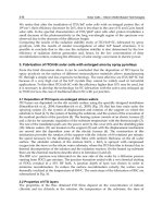
Fig. 10 shows an example of a “radially isometric orientation” where parameters of the robot
as listed in Table 1 are used.
For the controller that will be described later, the control input is determined using the value of
the radially isometric orientation, β. As shown in Equation 44, an integral is needed to obtain
the value of β. This implies that a controller using the value of β needs an integral calculation
every control cycle to obtain the value of β. This control scheme is thus undesirable for a
spacecraft equipped with limited on-board computational resources.
In order to reduce the effect of such limited on-board computation resources, we consider an
approximation of the “radially isometric orientation,” or simply, manifold.
Although it depends on the mass and the moment of inertia of the space robot, as shown in Fig.
10, the invariant manifold can be approximated by a plane surface around the goal link angles.
Any set of link angles around the goal link angles,
ˆ

x =

ˆ
φ
1
,
ˆ
φ
2
,

ˆ
θ

T
, can be approximated by a
linear combination of h
1
(φ
1d
,φ
2d
) and h
2
(φ
1d
,φ
2d
)
⎡
⎣
ˆ
φ
1
ˆ
φ
2
h
1
(φ
1d

,φ
2d
)
ˆ
φ
1
+ h
2
(φ
1d
,φ
2d
)
ˆ
φ
2
⎤
⎦
(46)
Fig. 11 shows a manifold approximated by a plane surface. It should be noted that if a set of
link angles is far away from the goal link angles, the difference between the approximating
manifold and the exact manifold, of course, becomes larger. Therefore, if a more accurate
approximate manifold is required, types of surfaces other than plane surfaces, such as spline
surfaces, should be used. However, we need a trade off between accuracy and computational
cost. In this chapter, taking into consideration experiments that will be discussed later, we use
an approximating manifold that is a plane surface.
2.3 Invariant manifold based control
2.3.1 Smooth time invariant feedback control
The control method proposed in (Mukherjee & Kamon, 1999) is given by
˙

r
= αr

ρ
2
tanh

n
1
β
2

−r
2

(47)
˙
ϕ
= −n
2
sgn
(
h
3
(φ
1d
,φ
2d
)
)

tanh
(
n
3
β
)
(48)
where α, n
1
,n
2
,n
3
, and ρ are positive scalar constants, and the link angle velocities are driven
by Equations 42 and 43.
510
Advances in Spacecraft Technologies
Applications of Optimal Trajectory Planning and
Invariant Manifold Based Control for Robotic Systems in Space
15
−4
−2
0
2
4
−4
−3
−2
−1
0

1
2
3
4
−0.6
−0.4
−0.2
0
0.2
0.4
0.6
0.8
1
1.2
1.4
2
[rad]
1
[rad]
[rad]
Fig. 10. Invariant manifold.
This control method is asymptotically stable, because as the value of β approaches zero, the
radius r, and the phase argument ϕ driven by the above control method approach zero. This
−4
−2
0
2
4
−4
−3

−2
−1
0
1
2
3
4
−0.6
−0.4
−0.2
0
0.2
0.4
0.6
0.8
1
1.2
1.4
2
[rad]
1
[rad]
[rad]
Fig. 11. Plane surface approximation of the invariant manifold.
511
Applications of Optimal Trajectory Planning
and Invariant Manifold Based Control for Robotic Systems in Space
16 Advances in Spacecraft Technologies
control method, however, suffers from slow convergence, and we now explain the reason for
this.

When β approaches zero, the control method (47) is equivalent to
˙
r
= −αr
3
(49)
This implies that the radius r does not converge to zero at a first-order convergence rate. In
addition, as β approaches zero, the change of phase argumentation, that is, the Lie bracket
motion, also becomes slower. As a result, the rate of convergence to approach the goal state
becomes very slow.
Furthermore, modeling errors were not considered in (Mukherjee & Kamon, 1999). The time
invariant feedback control method cannot stabilize the state to the goal state in the presence
of modeling errors, because the actual manifold is different from the manifold based on the
mathematical model.
2.3.2 Adaptive manifold based switching control
To overcome the disadvantages of the time invariant feedback controller, an adaptive
manifold based switching control is proposed here.(Kojima & Kasahara, 2010)
Firstly, the control method in the absence of modeling errors and time delay is explained as a
basic controller; then advanced functions are introduced. The basic control method consists
of two steps.
In the first step, in order to change the attitude of the main body as much as possible, Lie
bracket motion is actively utilized. For this purpose, until the state reaches the invariant
manifold, the radius r and the phase argument velocity
˙
ϕ are controlled to be constant:
˙
r
= 0, (50)
˙
ϕ

= −n
4
sgn(h
3
(φ
1d
,φ
2d
))sgn(β). (51)
If a trajectory of the link angles crosses the zero holonomy curve under the condition of
constant radius, as presented in (Hokamoto & Funasako, 2007), virtual goal link angles,
which asymptotically reach the goal angles, are set for the link trajectory not to cross the zero
holonomy curve.
In the second step, the state variables slide along the manifold until they reach the goal states.
In this step, in order for the radius r to converge to zero at a first-order convergence rate, the
radius is controlled by
˙
r
= −dr (52)
We can expect a fast convergence rate from Equations 50, 51 and 52, compared with the smooth
time invariant feedback control. This expectation will be verified experimentally.
The control input determined by the smooth invariant feedback control(Mukherjee & Kamon,
1999) is smooth, whereas the proposed control method is a switching control. This proposed
switching control, therefore, may induce undesirable oscillations on flexible appendages
attached to the main body or links.
Undesirable oscillations could be avoided by controlling the phase argument velocity
˙
ϕ so
that the connection from Equation 51 to Equation 48 becomes smooth as β approaches the
manifold. In this study, a smooth connection has not yet been investigated, and thus it remains

a future topic for study.
Next, let us consider an adaptive law to estimate the modeling error in the absence of a time
delay. In this study, we assume that there exists only a difference between the mathematical
512
Advances in Spacecraft Technologies
Applications of Optimal Trajectory Planning and
Invariant Manifold Based Control for Robotic Systems in Space
17
moment of inertia of the main body and the correct one, which is treated as a modeling error.
If an angular acceleration sensor is installed on the main body, and the link angles are driven
by the torque motors, then the moment of inertia of the main body can be directly estimated
from the relation between the torques and the angular acceleration. However, the link angles
of the model treated in this study are controlled in terms of the angular velocity. This implies
that the moment of inertia of the main body cannot be directly estimated using the relation
between the torque and the angular acceleration.
We are assuming here that the attitude of the main body can be measured by an attitude sensor
such as a magnetometer. We consider an adaptive law to estimate the moment of inertia of
the main body from the difference between the predicted attitude change and the actual one.
Let the error of the moment of inertia of the main body be given by
ΔJ
0
= J
0
−
ˆ
J
0
, (53)
where J
0

and
ˆ
J
0
are the correct and estimated moments of inertia of the main body,
respectively. The attitude change of the main body per one period of δϕ
= 2π is given by
Δθ
=

r=const
h
1
(r, ϕ, J
0
) dφ
1
(r, ϕ)+h
2
(r, ϕ, J
0
) dφ
2
(r, ϕ) (54)
The above path integral can be converted into a surface integral using Stokes’s theorem, Recall
that the modeling error given by Equation 53, Equation 54 can be approximated as follows:
Δθ
=

r=const

h
3
(r, ϕ, J
0
)dφ
1
∧ dφ
2


r=const
h
3
(r, ϕ,
ˆ
J
0
)dφ
1
∧ dφ
2
+

r=const
∂h
3
(r, ϕ, J
0
)
∂J

0




J
0
=
ˆ
J
0
ΔJ
0
dφ
1
∧dφ
2
(55)
The attitude change of the main body corresponding to the assumed moment of inertia of the
main body
ˆ
J
0
is given by
Δ
ˆ
θ :
=

r=const

h
3
(r, ϕ,
ˆ
J
0
) dφ
1
∧dφ
2
(56)
By comparing Equation 55 with Equation 56, the difference between the predicted and actual
attitude changes can be approximately represented by
Δθ
−Δ
ˆ
θ 

r=const
∂h
3
(r, ϕ, J
0
)
∂J
0





J
0
=
ˆ
J
0
ΔJ
0
dφ
1
∧dφ
2
(57)
Because the radius r is restricted to be constant during the first step in the proposed control
method, the surface area dφ
1
∧d φ
2
during one periodic motion of the phase argument δϕ = 2π
is always the same. Therefore, by solving Equation 57 with respect to the modeling error, we
have
Δ
ˆ
J
0

Δθ − Δ
ˆ
θ


r=const
∂h
3
(r,ϕ,J
0
)
∂J
0



J
0
=
ˆ
J
0
dφ
1
∧dφ
2
(58)
513
Applications of Optimal Trajectory Planning
and Invariant Manifold Based Control for Robotic Systems in Space
18 Advances in Spacecraft Technologies
Using this relation, the actual moment of inertia of the main body can be estimated as
J
0
=

ˆ
J
0
+ Δ
ˆ
J
0
(59)
The denominator of Equation 58 is, however, based on the estimated moment of inertia of the
main body, which is not yet equivalent to the actual one. Therefore, if the moment of inertia
of the main body is simply updated, based on Equation 59, the estimated moment of inertia
might become a meaningless (e.g., negative) value in a physical sense. In order to avoid such
a situation, Equation 59 is replaced with
J
0
=
ˆ
J
0
+ γΔ
ˆ
J
0
(0 < γ < 1) (60)
to update the estimated moment of inertia.
We explain the value that is selected for γ in this study. In general, the smaller the value of
γ and the greater the number of estimations chosen, then the more accurate the estimation
could be, whereas a long time is required to obtain an accurate moment of inertia.
Suppose that the estimated moment of inertia approaches the actual moment after ten
estimations. In this case, it may be natural to set γ to 0.1

(= 1/10). For greater safety, half
this value, i.e., 0.05, is chosen for γ.
In addition, a value, which is surely less than the actual one, is chosen as the initial guess
for the moment of inertia so that the estimated moment of inertia is unlikely to decrease or
become negative, but instead increases during updates.
Next, we consider a case where a time delay exists. In this study, we assume that a time delay
exists only for the output, but not in the control input, and that this time delay does not vary,
but instead, is always constant.
Because the control method tries to control the link angles so that the radius r and the phase
argument velocity
˙
ϕ are kept constant during the first step, if no time delay exists in the
output, the vector of the link angle motion is always tangential to the vector from the goal
angles to the current link angles, and thus the radius r never changes.
On the other hand, if a time delay τ exists, a phase argument difference τ
˙
ϕ occurs between the
measured link angles B
(
ˆ
φ
1
(t −τ),
ˆ
φ
2
(t −τ)) and the actual link angles A(
ˆ
φ
1

(t),
ˆ
φ
2
(t)), which
corresponds to the time delay τ, as shown in Fig. 12. In this case, the vector of link angles
velocity is determined as

b, based on the measured link angles B. This vector differs from
the desired velocity vector

a which is determined in the absence of time delay. The phase
argument difference results in a radius increase Δr. Taking this fact into consideration, we
introduce here a method for estimating the time delay from radius changes.
Suppose that the radius at link angles A is the same as that of B. In this case, both vectors

a and

b have the same length r
˙
ϕ, as shown in Fig. 12. Taking into account that the angle between
these two vectors corresponds to τ
˙
ϕ, the radius increase can be approximately expressed as
˙
r
= r
˙
ϕtan(τ
˙

ϕ) (61)
From this relation, using the radius increase Δr during a specified time duration Δt, the time
delay τ can be estimated as
τ
=

1

˙
ϕ

tan
−1

Δr

r
˙
ϕΔt

(62)
Note that the radius r at the link angles A is not always the same as that at the measured link
angles B due to the effect of the past control input, thus, the estimation of the time delay should
be updated using Equation 62 several times. In this study, the time delay was estimated every
phase argument change of δϕ
= π/4 during the first step.
514
Advances in Spacecraft Technologies
Applications of Optimal Trajectory Planning and
Invariant Manifold Based Control for Robotic Systems in Space

19
r
.
.
1
(t))
2
(t),
1
r
r
.
goal
.
2
A
B
(
(
t- ),
2(t-
))
a
b
b
Fig. 12. Schematic representation of relation between the time delay and the radius change.
Until the next estimation of the time delay, the current attitude of the main body, the link
angles (A in Fig. 12), and the radius r are predicted using the history of the past control input
corresponding to the estimated time delay.
Then the new value for the control input is determined using the predicted current state. At

the next estimation of the time delay, it is updated by inspecting the difference between the
predicted radius and the actual one.
2.4 Experimental verification
2.4.1 Experimental setup
Fig. 13 shows the experimental setup of a planar two-link space robot. This robot was
equipped with a magnetometer to sense the attitude of the main body, two stepper motors
to drive each link angle, and two encoders to sense each link angle. Note that operational
angle of each link was restricted within
±110 deg due to structural limitations.
Fig. 13. Experimental apparatus for the planar two-link robot.
515
Applications of Optimal Trajectory Planning
and Invariant Manifold Based Control for Robotic Systems in Space
20 Advances in Spacecraft Technologies
m
0
2.280 kg
m
1
0.922 kg
m
2
0.493 kg
l
01
0.125 m
l
11
0.283 m
l

12
0.017 m
l
21
0.270 m
J
0
0.03585 kgm
2
J
1
0.00410 kgm
2
J
2
0.00324 kgm
2
Table 1. Robot parameters.
A large glass board, called a flight-bed, was horizontally placed. To imitate microgravity, the
surface of the board was paved with a number of ball bearings to decrease frictional drag.
Note that friction due to the ball bearings was about 0.019 G, which is much greater than that
of air bearings. The ball bearings, therefore, will have to be replaced with air bearings in the
near future.
Because noise was included in the attitude output from the magnetometer, a low-pass filter,
whose time-lag does not have an impact on the attitude measurement, was implemented, to
cut off the noise. A personal desktop computer (PC) equipped with a digital board was placed
next to the board. The PC measured the state of the robot via the board, determined the control
input (link angular velocities) based on the control law implemented in the C language, and
drove the stepper motors situated on the link joints. The sampling and control cycle is 100
msec.

The mass of each link was measured by an electro balance, and the moment of inertia of each
link was measured by a moment of inertia measurement device, MOI-005-104 from the Inertia
Dynamics and the LLC Co.
The moment of inertia of the main body was measured around the center of mass, while the
moment of inertia of each link was measured around the joint part, and then converted to one
around the mass center. The parameters of the experimental setup are as listed in Table 1.
2.4.2 Experimental results
Experiments were carried out on smooth invariant feedback control and the proposed
adaptive invariant manifold based switching control using the parameters listed in Table 2.
Then their convergence rates as they approached the goal state were compared in the presence
of both modeling error and time delay.
Gains α = 0.2,0.4, n
1
= 1.0,n
2
= 2.0,n
3
= 1.0
n
4
= π/5,d = 0.2,γ = 0.05
Initial state φ
1
= φ
2
= θ = 0.3 rad
Goal state φ
1d
= φ
2d

= 0.6 rad, θ
d
= 0.2 rad
Initial estimated moment of inertia
ˆ
J
0
= 0.015 kgm
2
Table 2. Experimental conditions.
516
Advances in Spacecraft Technologies
Applications of Optimal Trajectory Planning and
Invariant Manifold Based Control for Robotic Systems in Space
21
Taking into consideration that the magnetometric sensor output included noise of
approximately 2 deg, the tolerance of the judgment of attainment with regard to the invariant
manifold and the convergence criterion to the goal value were set to 2 deg in the mean square
root of the second power of angle errors. The time delay was set to 0.5 sec, and implemented
by feeding the controller the output measured five sampling cycles previously. The initial
guess for the moment of inertia was set to 0.015 kgm
2
, which is surely less than the actual
value. We explain the results below.
Two results for the smooth invariant feedback control are shown in Figs. 14(a) and 14(b).
These correspond to the results for control gains of α
= 0.4, and α = 0.2, respectively. The
results of the proposed control method are shown in Figs. 15 to 17. Figs. 15, 16, and 17 show
the time responses of the state variables, the estimated time delay, and the estimated moment
of inertia of the main body, respectively.

The link angle φ
1
controlled by the smooth invariant feedback control exceeded the link angle
limitation around 4 sec for the case of a control gain with α
= 0.4. This is because the phase
argument velocity
˙
ϕ was very large, and the phase argument error due to time delay was also
very large, thus leading to radius divergence, as explained in Fig. 12.
Contrary to the above case, for the case of the control gain α
= 0.2, which is less than that of
the above case, the phase argument velocity
˙
ϕ became smaller, the phase argument error due
to time delay became smaller, which led to a smaller divergence rate of the link angles. As the
result, the link angles did not exceed the angle limitation. Although the link angles reached
the goal link angles, the attitude of the main body did not converge to the goal attitude. This is
because β based on the mathematical model was incorrect, due to the error in the moment of
inertia, and after determining that β approached zero, the link angles, which were controlled
by the controller without any adaptive law to compensate for the error, moved to the goal
angles(φ
1d
,φ
2d
) directly, and finally converged to other state. In addition, it took a long time
for the link angles to move directly to the goal link angles (φ
1d
,φ
2d
) in the second step, because

the control law almost became
˙
r
= −αr
3
, for which the convergence rate was not of first order
as β approached zero.
On the other hand, the proposed control method succeeded in controlling so as to move the
states to the goal states, and the estimated time delay and moment of inertia converged to 0.77
sec, and 0.0244 kgm
2
, respectively.
The estimated moment of inertia of the main body was slightly less than the actual one. This
may be because additional torque was generated due to friction between the ball bearings and
the arms, which prevented the links from moving in the ideal motion, and in turn induced
greater than the ideal attitude reaction of the main body, which resulted in an interpretation
of the moment of inertia to be less than the actual one.
As shown in Fig. 16, the estimated time delay, 0.77 sec, was slightly greater than the actual
time delay, that is, 0.5 sec. However, from Fig. 15, we can justify the estimated time delay
because after the time delay was estimated, the magnitude of sinuous motion of the link angle
φ
1
around the goal angle was the same as that of φ
2
for the period between 8 and 14 sec.
In other words, it can be said that the radius r did not change; thus the states were almost
correctly predicted.
After the time delay was estimated, the link angles changed their sinuous motion to straight
line motion at a time of around 14 sec, in order to approach the goal angles at a first-order
convergence rate, as shown in Fig. 15. This implies that the state approached the invariant

manifold around the above time, and at that time the control logic changed from the first step
to the second step.
517
Applications of Optimal Trajectory Planning
and Invariant Manifold Based Control for Robotic Systems in Space
22 Advances in Spacecraft Technologies
-0.5
0
0.5
1
1.5
0 5 10 15 20 25 30 35 40
angle [rad]
time
[
s
]
(a) α = 0.4
-0.5
0
0.5
1
1.5
0 5 10 15 20 25 30 35 40
angle [rad]
time
[
s
]
(b) α = 0.2

Fig. 14. Time responses of the state variables resulting from smooth invariant feedback
control
In addition, Fig. 15 shows that the link motion returned to a sinuous motion at around 25
sec. This implies that even as the link angles were controlled to slide on the manifold, β left
the convergence tolerance due to the moment of inertia error of the main body, and then the
control logic returned to the first step.
We can observe in Fig. 17 that since the control logic returned to the first step, the adaptive
law to estimate the moment of inertia of the main body re-functioned, the moment of inertia
was updated towards the correct value at around 30 sec, and this update contributed to the
state convergence to the goal state.
Consequently, the effectiveness of the proposed control method was validated by comparing
the results of the smooth invariant feedback control method with those of the proposed control
method.
518
Advances in Spacecraft Technologies
Applications of Optimal Trajectory Planning and
Invariant Manifold Based Control for Robotic Systems in Space
23
3. Conclusion
This Chapter presents two main topics related to the space robotic systems: (1) Optimal
trajectory planning for two-link robotic arm manipulators in the presence of chaotic
wandering obstacles and (2) Invariant manifold based control methods for spacecraft attitude
control problems.
The first Section describes mathematical modeling of a two-link robotic manipulator in
three-dimensional space using Lagrange equations. The system includes three rotational
joints (RRR) and a point mass payload at the end effector. To ensure collision avoidance,
the path -12constraints are formulated based on the projected obstacle’s position along the
arms of the robot. The associated non-linear optimization problems were formulated and
solved using the Chebyshev-pseudospectral method. It should be stressed out that, the
method presented in the current work allows not only to minimize the specified arbitrary

non-linear cost function, but also allows to solve the optimization task in view of multiple
additional non-linear constraints that the user of the robotic systems may choose to impose
based on mission requirements or considerations. In the current work a procedure of optimal
path planning for rigid manipulators performing operations in presence of the wandering
obstacles, changing their positions and shapes, has been successfully implemented. The
optimal scenarios enable to perform deployment of the payloads avoiding their collision
with the non-statioary obstacles. It has been demonstrated that the actuator efforts required
to perform the task is higher than for the similar cases without the obstructing obstacles.
Examples of additional constraints may involve path constraints on the system, prohibiting
the members to enter a specified space area or, on the contrary, prescribing the system to
follow the desired trajectory or prescribing for the members of the robotic system not to leave
the allowed bandwidth corridors. The method is generic and is not restricted to the listed
examples of the cost functions and additional constraints.
In the second Section, an adaptive invariant manifold based switching control has been
proposed for controlling a planar two-link space robot. The proposed control method is a kind
of invariant manifold based control, and has two advanced functions: estimation of the time
delay in the system, and estimation of the moment of inertia of the main body. The proposed
-0.5
0
0.5
1
1.5
0 5 10 15 20 25 30 35 40
angle [rad]
time
[
s
]
Fig. 15. Time responses of the state variables for the case of adaptive invariant manifold
switching control.

519
Applications of Optimal Trajectory Planning
and Invariant Manifold Based Control for Robotic Systems in Space
24 Advances in Spacecraft Technologies
0
0.2
0.4
0.6
0.8
1
1.2
1.4
0 5 10 15 20 25 30 35 40
estimated delay time [s]
time
[
s
]
Fig. 16. Time response of the estimated time delay.
control method consists of two steps. In the first step, link angles are controlled to carry out
Lie bracket motion so that the attitude of the main body approaches the invariant manifold
as much as possible. In addition, the time delay and the modeling error due to the moment
of inertia are estimated. During the first step, provided that a time delay does not exist, the
control method manages to control the link angles so that the distance between the current
link angles and goal link angles, that is, the radius, is kept constant. The radius does however
change, due to the time delay. Taking into consideration the relation between the change of
radius and the time delay, the time delay is estimated from the change in the radius. After
estimating the time delay, a modeling error, which is taken to be the difference between the
accurate and the estimated moments of inertia of the main body, is estimated by comparing
the predicted attitude change of the main body and the actual one, and then the mathematical

moment of inertia is updated. In the second step, the link angles are controlled to slide on the
invariant manifold until it converges to the goal state. The effectiveness of the functions of the
proposed control scheme method, the reduction in convergence time compared to the smooth
0
0.005
0.01
0.015
0.02
0.025
0.03
0.035
0.04
0 5 10 15 20 25 30 35 40
estimated moment of inertia [kgm ]
time
[
s
]
Fig. 17. Time response of the estimated moment of inertia of the main body.
520
Advances in Spacecraft Technologies
Applications of Optimal Trajectory Planning and
Invariant Manifold Based Control for Robotic Systems in Space
25
invariant feedback control, and estimation of not only the time delay, but also the modeling
errors, were successfully verified experimentally.
4. References
Brockett, R. (1983). Differential Geometric Control Theory, Asymptotic Stability and Feedback
Stabilization, Birkhauser, Boston.
Cao, B., Dodds, G. & Irwin, G. (1997). Constrained time-efficient and smooth cubic

spline trajectory generation for industrial robots, Control Theory and Applications, IEE
Proceedings - 144(5): 467 –475.
Cerven, W. T. & Coverstone, V. L. (2001). Optimal reorientation of a multibody spacecraft
through joint motion using averaging theory, Journal of Guidance, Control and
Dynamics 24(4): 788–795.
Gil, P., Murray, W. & Saunders, M. (2002). User’s Guide for SNOPT, Version 6: A FORTRAN
Package for Large-Scale Nonlinear Programming, University of California, San Diego,
CA.
Hashimoto, T., F. A. H. & Amemiya, T. (2006). Simultaneous feedback stabilization of space
robot attitude, J. Japan Soc. Aero. Space Sci. 54(635): 549–554.
Hokamoto, S. & Funasako, T. (2007). Feedback control of a planar space robot using a moving
manifold, Journal of Robotic Society of Japan 25(5): 95–101.
Hu, S., Xue, L., Xu, W., Qiang, W. & Liang, B. (2008). Trajectory planning of space robot
system for reorientation after capturing target, Systems and Control in Aerospace and
Astronautics, 2008. ISSCAA 2008. 2nd International Symposium on, pp. 1–6.
Huang, P. & Xu, Y. (2006). Pso-based time-optimal trajectory planning for space robot with
dynamic constraints, Robotics and Biomimetics, 2006. ROBIO ’06. IEEE International
Conference on, Kunming, China, pp. 1402–1407.
Kojima, H. & Kasahara, S. (2010). Adaptive invariant manifold based switching control for
planar two-link space robot(2nd report), J. Japan Soc. Aero. Space Sci. 58(679): 233–238.
Luo, J. & Tsiotras, P. (1998). Exponentially convergent control laws for nonholonomic systems
in power form, Systems & Control Letters 35(2): 87–95.
Luo, X., Fan, X., Zhang, H. & Chen, T. (2004). Integrated optimization of trajectory planning
for robot manipulators based on intensified evolutionary programming, Robotics and
Biomimetics, 2004. ROBIO 2004. IEEE International Conference on, pp. 546 –551.
Mukherjee, R. & Kamon, M. (1999). Almost smooth time-invariant control of planar space
multibody systems, Robotics and Automation, IEEE Transactions on 15(2): 268–280.
Pomet, J. B. (1992). Explicit design of time-varying stabilization control law for a class of
controllable systems without drift, Systems & Control Letters 18(2): 147–158.
Reyhanoglu, M. & McClamroch, H. H. (1992). Planar reorientation maneuvers of space

multibody systems using internal controls, Journal of Guidance, Control, and Dynamics
15(6): 1475–1480.
Samson, C. (1995). Control of chained systems application to path following and time-varying
point- stabilization of mobile robots, Automatic Control, IEEE Transactions on
40(1): 64–77.
Seshadri, C. & Ghosh, A. (1993). Optimum path planning for robot manipulators amid static
and dynamic obstacles, Systems, Man and Cybernetics, IEEE Transactions on 23(2): 576
–584.
Sordalen, O. & Egeland, O. (1995). Exponential stabilization of nonholonomic chained
systems, Automatic Control, IEEE Transactions on 40(1): 35–49.
521
Applications of Optimal Trajectory Planning
and Invariant Manifold Based Control for Robotic Systems in Space
26 Advances in Spacecraft Technologies
Teel, A. R., M. R. M. & Walsh, G. C. (1995). Nonholonomic control systems: From steering to
stabilization with simusids, International Journal of Control 62(4): 849–870.
Trivailo, P. M. (2007). Collision-free trajectory planning for 2d and 3d robotic
arm manipulators in the presence of mobile wandering obstacles - paper
iac-07-c2.3.02., 58th International Astronautical Federation Congress, Hyderabad,
India, pp. 4952–4960.
Vannoy, J. & Xiao, J. (2008). Real-time adaptive motion planning (ramp) of mobile
manipulators in dynamic environments with unforeseen changes, Robotics, IEEE
Transactions on 24(5): 1199–1212.
Williams, P. (2005). User’s Guide to DIRECT, Version 1.17, RMIT Technical Report, Melbourne,
Australia.
Williams, P., Trivailo, P. M. & Lee, K. W. (2009). Real-time optimal collision-free control for
robotic arm manipulators in the presence of wandering obstacles, 60th International
Astronautical Congress, Vol. 7, pp. 5500–5508.
Xu, W., Li, C., Liang, B., Xu, Y., Liu, Y. & Qiang, W. (2009). Target berthing and
base reorientation of free-floating space robotic system after capturing, ACTA

ASTRONAUTICA 64(2-3): 109–126.
Yamada, K. (1994). Attitude control of space robot by arm motion, Journal of Guidance, Control,
and Dynamics 17(5): 1050–1054.
Yoshida, E., Esteves, C., Belousov, I., Laumond, J P., Sakaguchi, T. & Yokoi, K. (2008). Planning
3-d collision-free dynamic robotic motion through iterative reshaping, Robotics, IEEE
Transactions on 24(5): 1186–1198.
522
Advances in Spacecraft Technologies
23
Optimal Control Techniques for Spacecraft
Attitude Maneuvers
Shifeng Zhang, Shan Qian and Lijun Zhang
National University of Defense Technology,
P. R. China
0B1. Introduction
The capability of attitude maneuvers and attitude tracking for spacecrafts is required in the
current sophisticated space missions. In short, it is to obtain command requirements and
attitude orientation after some form of control. With the development of space missions, the
ability of rapid and energy-saved large-angle attitude maneuvers is actively expected. And
the high requirements for the attitude control design system are increasingly demanded.
Consequently, optimal control for attitude maneuvers has become an important research
direction in the aerospace control area.
From control aspect, spacecraft attitude maneuvers mainly involve trajectory planning
(Guidance), attitude determination (Navigation), and attitude control (Control). Further
researches about these three key technologies are necessary to achieve optimal control for
attitude maneuvers. In this chapter, the necessary background on optimal control for
attitude maneuvers of three-axis stabilized spacecraft is provided, and the recent work
about guidance and navigation as well as control is summarized, which is presented from
three parts as follows:
1. The optimal trajectory planning method for minimal energy maneuvering control

problem (MEMCP) of a rigid spacecraft;
2. Attitude determination algorithm based on the improved gyro-drift model;
3. Attitude control of three-axis stabilized spacecraft with momentum wheel system.
1B2. Optimal trajectory planning method for MEMCP of a rigid spacecraft
The trajectory planning for attitude maneuvers is to determine the standard trajectory for
spacecraft attitude maneuvers with multi-constraints using optimization algorithm, which
makes the spacecraft move from the initial state to the anticipated state within the specified
period and optimizes the given performance index. At present, the optimal trajectory
planning problems for spacecraft attitude maneuver mainly focus on the time-optimal and
fuel-optimal control. A fuel-optimal reorientation attitude control scheme for symmetrical
spacecraft with independent three-axis controls is derived in (Li & Bainum, 1994). Based on
the low-thrust gas jet model and Euler’s rotational equation of motion, Junkins and Turner

(Junkins & Turner, 1980) investigate the optimal attitude control problem with multi-axis
maneuvers. They use the closed-form solution of the single-axis maneuver as an initial value
and minimize the quadratic sum of the integral of the control torques. Vadali and Junkins
(Vadali & Junkins, 1984) have addressed the large-angle reorientation optimal attitude
Advances in Spacecraft Technologies

524
control problem for asymmetric rigid spacecraft with multiple reaction wheels by using an
integral of a weighted quadratic function associated with controlled variables as loss
function. Further more, Vadali and Junkins (Vadali & Junkins, 1983) also investigate the
optimal attitude maneuvering control problem of rigid vehicles.
The complete optimal attitude control problem is essentially a two-point boundary value
problem. Since the input variables of the control system are restricted, Pontryagin’s
Minimum Principle (PMP) is usually used to solve the optimal attitude control problem of
the symmetric or asymmetric rigid spacecraft with constraints. The optimal attitude control
problem with fixed maneuvering period has been solved in (Vadali & Junkins, 1984; Vadali
& Junkins, 1983; Dwyer, 1982; Schaub & Junkins, 1997). In practice, numerical methods are

generally used to solve the highly nonlinear and close coupling differential equations
derived from PMP. However, the method falls short to deal with dynamic optimization
problem with uncertain terminal time, and the shooting method is commonly adopted
whereas it will increase the iterations and computational burden. Therefore, the satisfied
development has not yet been achieved for large-angle attitude reorientation of asymmetric
rigid spacecraft up to now.
Recently, (Chung & Wu, 1992) presents a nonlinear programming (NLP) method to solve
time-optimal control problem for linear system. Different from the conventional shooting
method which sets the time step as a fixed value, the NLP method considers the time step as
a variable and obtains the optimal solution on the premise of ensuring sufficient
discretization precision of the model. (Yang et al., 2007) further discusses MEMCP of a rigid
spacecraft, which introduces two aspects of research on the three-axis spacecraft with
limited output torque, including: 1) the description of MEMCP using NLP method, and 2)
the construction method for initial feasible solution of the NLP. However, the derivation in
that paper has some errors and the initial feasible solution does not conform to the actual
motion of the spacecraft. Moreover, the method augments the optimizing time and the
randomness of the variation between the adjacent attitude commands. Consequently, this
section (Zhang et al., 2009) further improves the proposed method and presents a new
construction method for initial feasible solution of the NLP, and obtains the optimal control
period and torques by the energy-optimal criterion. Simulation results demonstrate the
feasibility and advantages of the improved method.
2.1 Dynamical and kinematical equations of a rigid spacecraft
The attitude motion of a spacecraft can be described by its dynamical and kinematical
equations. In general, the dynamic equation of motion can be represented as

1111
2222
3333
1/ 0 0 0 ( ) /
01/ 0 0 ( ) /

001/ 0 () /
xx zyxx x
yyzxyy y
zzyxzzz
IIIITI
IIIITI
IIIITI
ωωωωω
ωωωωω
ωωωωω
−+
=− − × + + −
−+
⎡⎤
⎧⎫
⎡⎤ ⎡ ⎤ ⎡ ⎤⎡ ⎤ ⎡ ⎤
⎢⎥
⎪⎪
⎢⎥ ⎢ ⎥ ⎢ ⎥⎢ ⎥ ⎢ ⎥
⎨⎬
⎢⎥
⎢⎥ ⎢ ⎥ ⎢ ⎥⎢ ⎥ ⎢ ⎥
⎪⎪
⎢⎥
⎢⎥ ⎢ ⎥ ⎢ ⎥⎢ ⎥ ⎢ ⎥
⎣⎦ ⎣ ⎦ ⎣ ⎦⎣ ⎦ ⎣ ⎦
⎩⎭
⎣⎦




(1)
where
x
I ,
y
I
,
z
I and
1
I ,
2
I ,
3
I denote the moment of inertia of rigid spacecraft about the
principal axis and the three reaction wheels, respectively. ,,
x
y
z
ω
ωω
are the components of
spacecraft’s angular velocity expressed in its body-fixed frame, and
123
,,
ω
ωω
are the
components of the reaction wheel’s angular velocity.

123
,,TTTare the control torques
provided by the perpendicular momentum wheels along the principal axis.
The equation of angular motion of the momentum wheels can be obtained from Eq.(1)
Optimal Control Techniques for Spacecraft Attitude Maneuvers

525

1 111 11
2 222 22
3 333 33
1/ 0 0 0 ( ) (1/ 1/ )
0 1/ 0 0 ( ) (1/ 1/ )
0 0 1/ 0 ( ) (1/ 1/ )
xzyxxx
yzxyy y
zyx z z z
IIIIIIT
IIIIIIT
IIIIIIT
ωωωωω
ωωωωω
ωωωωω
−+ +
=−×++++
−+ +
⎡⎤
⎧⎫
⎡⎤⎡ ⎤ ⎡ ⎤⎡ ⎤ ⎡ ⎤
⎢⎥

⎪⎪
⎢⎥⎢ ⎥ ⎢ ⎥⎢ ⎥ ⎢ ⎥
⎨⎬
⎢⎥
⎢⎥⎢ ⎥ ⎢ ⎥⎢ ⎥ ⎢ ⎥
⎪⎪
⎢⎥
⎢⎥⎢ ⎥ ⎢ ⎥⎢ ⎥ ⎢ ⎥
⎣⎦⎣ ⎦ ⎣ ⎦⎣ ⎦ ⎣ ⎦
⎩⎭
⎣⎦



(2)

Considering the 1-2-3 sequence of rotations, the kinematic equation of motion using Euler
angle representation is given by

sec cos sec sin 0
sin cos 0
tan cos tan sin 1
x
y
z
φθψθψω
θψ ψω
ψ
θψ θψ ω
−

=
−
⎡⎤
⎡
⎤⎡ ⎤
⎢⎥
⎢
⎥⎢ ⎥
⎢⎥
⎢
⎥⎢ ⎥
⎢⎥
⎢
⎥⎢ ⎥
⎣
⎦⎣ ⎦
⎣⎦



(3)

where
ϕ
is roll angle,
θ
is pitch angle and
ψ
is yaw angle.
2.2 Modeling and analysis of MEMCP

The MEMCP of the rigid spacecraft between two attitudes can be described as an optimizing
problem as follows.
The initial attitude is given by

initial initial initial
1 2 3 1,initial 2,initial 3,initial
( (0), (0), (0)) ( , , )
( (0), (0), (0)) (0,0,0)
( (0), (0), (0)) ( , , )
xyz
φθψ φ θ ψ
ωωω
ωωω ω ω ω
=
⎧
⎪
=
⎨
⎪
=
⎩
(4)

The goal is to determine the control inputs
T
123
() [ (), (), ()]t TtTtTt=T for some [0, ]
f
tt∈ to
minimize the following objective function

3
222 2
123
1
00
(() () ()) ()
ff
tt
k
k
JTtTtTtdt Ttdt
=
=++=
∑
∫∫


subject to

final final final
,min ,max
(( ),( ), ( )) ( , , )
( ( ), ( ), ( )) (0,0,0)
( ) , for [0, ], 1,2,3
ff f
xf yf zf
iii f
tt t
ttt

TTtT tti
φθψ φθψ
ωωω
=
=
≤≤ ∈ =
(5)

where
initial initial initial
(,, )
φθψ
and
final final final
(,, )
φθψ
represent the initial and desired final
attitudes of the spacecraft, respectively.
f
t
is determined by the optimization process.
Due to the characteristics of highly nonlinear and close coupling of the problem, it will be
solved in the discrete-time domain using numerical method. First, we divide the interval
[0, ]
f
tt∈ into N equidistant subinterval and assume that the angular acceleration is
constant in each subinterval. Therefore, from Eq.(1) and Eq.(2), we can obtain
Advances in Spacecraft Technologies

526

1
0
111
222
333
0()()
() (0) 1/ 0 0
() (0) 0 1/ 0 ( ) 0 ( )
() () 0
() (0) 0 0 1/
( ) () ()
()()()
( ) () ()
zy
xx x
i
yy y z x
k
yx
zz z
xx
yy
zz
kk
iI
iIkk
kk
iI
II kI k

II kI k
II kI k
ωω
ωω
ωω ω ω
ωω
ωω
ωω
ωω
ωω
−
=
⎧
−
⎡⎤⎡ ⎤⎡ ⎤⎡ ⎤
⎪
⎢⎥⎢ ⎥⎢ ⎥⎢ ⎥
=
−−×
⎨
⎢⎥⎢ ⎥⎢ ⎥⎢ ⎥
⎪
⎢⎥⎢ ⎥⎢ ⎥⎢ ⎥
−
⎣⎦⎣ ⎦⎣ ⎦⎣ ⎦
⎩
⎡
++
++
++

∑
1
2
3
()/
()/
()/
x
y
z
Tk I
Tk I t
Tk I
⎫
⎤⎡ ⎤
⎪
⎢⎥⎢⎥
+
Δ
⎬
⎢⎥⎢⎥
⎪
⎢⎥⎢⎥
⎣⎦⎣⎦
⎭
(6)

11
1
22

0
33
111
222
333
() (0) 1/ 0 0 0 () ()
() (0) 0 1/ 0 ( ) 0 ( )
() (0) 0 0 1/ ( ) ( ) 0
( ) () ()
( ) () ()
( ) () ()
xzy
i
yz x
k
zyx
xx
yy
zz
iI kk
iIkk
iIkk
II kI k
II kI k
II kI k
ωω ωω
ωω ω ω
ωω ωω
ωω
ωω

ωω
−
=
−
=
+−×
−
++
++
++
⎧
⎡
⎤
⎡⎤⎡ ⎤⎡ ⎤
⎪
⎢
⎥
⎢⎥⎢ ⎥⎢ ⎥
⎨
⎢
⎥
⎢⎥⎢ ⎥⎢ ⎥
⎪
⎢
⎥
⎢⎥⎢ ⎥⎢ ⎥
⎣⎦⎣ ⎦⎣ ⎦
⎣
⎦
⎩

⎡
∑
1
2
3
1
2
3
()()
()()
()()
11
11
11
x
y
z
Tk
Tk t
Tk
II
II
II
+
++ Δ
+
⎫
⎡⎤
⎤
⎪

⎢⎥
⎢⎥
⎬
⎢⎥
⎢⎥
⎪
⎢⎥
⎢⎥
⎣⎦
⎣⎦
⎭
(7)
where
1
/
ii f
tt t t N
−
Δ= − =
,
1,2, ,iN
=

.
Suppose that the time derivative of
φ
,
θ
,
ψ

are constant during each subinterval, then we
have

1
0
() (0)
() (0)
() (0)
sec ( )cos ( ) sec ( )sin ( ) 0 ( )
sin ( ) cos ( ) 0 ( )
tan ( )cos ( ) tan ( )sin ( ) 1
()
i
k
x
y
z
i
i
i
kk kk k
kkkt
kk kk
k
φφ
θθ
ψψ
θψ θψ ω
ψψω
θψ θψ

ω
−
=
=+
⎡
⎤
−
⎡⎤
⎡⎤⎡ ⎤
⎢
⎥
⎢⎥
⎢⎥⎢ ⎥
Δ
⎢
⎥
⎢⎥
⎢⎥⎢ ⎥
⎢
⎥
⎢⎥
⎢⎥⎢ ⎥
−
⎣⎦⎣ ⎦
⎣⎦
⎣
⎦
∑
(8)

Therefore, the previous MEMCP can be described as a constrained NLP problem. Given the
initial attitudes, determine the values of (0), , ( 1)N
−
TT and t
Δ
to minimize

31
2
10
()
N
k
ki
JTit
−
==
=
Δ
∑∑

subject to

upper
final final final
,min ,max
0
( ( ), ( ), ( )) ( , , )
( ( ), ( ), ( )) (0,0,0)
() , 1,2,3; 0,1, , 1

xyz
iii
tt
NN N
NNN
TTjTi j N
ε
φθψ φθψ
ωωω
<<Δ<Δ
⎧
⎪
=
⎪
⎨
=
⎪
⎪
≤
≤== −
⎩

(9)

where
ε
is a small positive number to ensure the computation time is not excessively long.
The question is how to select the value of N to solve the discrete NLP problem mentioned
above. For the unconstrained linear programming problem, (Chung & Wu, 1992) points out
the initial value of N must be greater than the dimensions of the state variables, which is

adopted in this paper.
Optimal Control Techniques for Spacecraft Attitude Maneuvers

527
2.3 Construction of initial feasible solution of NLP problem
The NLP problem usually requires the initial feasible solution to start the optimization
process. The initial feasible solution is a set of optimization variables (0), , ( 1)N −TT and
tΔ which satisfy Eq.(9). Different initial feasible solutions will yield different local optimal
solutions, and the deviation of the initial feasible solution from the optimal solution will
affect the iteration times and computation time. (Yang et al., 2007) presents a construction
method of the initial feasible solution. However, the solution does not agree well with the
actual motion of the spacecraft, and the randomness of variation between the adjacent
attitude commands is excessively large. To solve this problem, a new construction of the
initial feasible is presented in this section.
The first step is to determine a maneuvering trajectory satisfying the boundary conditions
without the constraints of the control torques. Then, the set of control torques computed in
the above trajectory is checked. If it satisfies all the constraints, the set of control torques and
tΔ is the initial feasible solution. Otherwise, we need to adjust the velocity and acceleration
until finding a set of initial feasible solution.
With the given N , the attitude trajectories satisfying the boundary conditions can be
determined by

()
initial initial
final
final
0,1
2
(1) (1
() ()

2
2, , 1
, 1
ii
i
i
ii
ii
N
iN
iNN
φθ
γφ γ φ φ
φθ
φ
=
−
−+ − −
==
−
=−
=+
⎧
⎪
⎪
⎪
⎨
⎪
⎪
⎪

⎩

()
final
final
initial
0,1
2
(1) (1)
2
2, , 1
, 1
0,1
(
()
i
i
i
ii
N
iN
iNN
i
i
i
θγθθ
θ
ψ
ψ
ψ

=
−
−+ − −
−
=−
=+
=
−
=
⎧
⎪
⎪
⎪
⎨
⎪
⎪
⎪
⎩

()
final
final
2
1) ( 1)
2
2, , 1
, 1
i
i
i

N
iN
iNN
γψ ψ
ψ
−
+−−
−
=−
=+
⎧
⎪
⎪
⎪
⎨
⎪
⎪
⎪
⎩

(10)
where
i
γ
is a random number obeying the uniform distribution in the interval [0, 1] . Euler
angle vector is defined as
T
[,, ]
φ
θψ

=λ , and it is obvious that
(
)
i
λ
satisfies the initial
constraints in Eq.(4) and final constraints in Eq.(9).
Take the roll angle
φ
for example, we can easily obtain the inequalities
(1) ()
f
inal
ii
φ
φφ
−
≤≤

or ( 1) ( )
f
inal
ii
φ
φφ
−≥ ≥ . It is shown that the attitude trajectory
(
)
i
φ

constructed by the
previous model approaches the value of
f
inal
φ
all along. The process is not reciprocating and
in well agreement with the optimal maneuvering process.
Choose the appropriate value of t
Δ
to satisfy the constraint
upper
0 tt
ε
<
<Δ <Δ , so that

(1)()
()
(1)()
() 0,1, ,
()
(1) ()
ii
t
i
ii
iiN
t
i
ii

t
φφ
φ
θθ
θ
ψ
ψψ
+−
Δ
+−
==
Δ
+−
Δ
⎡⎤
⎢⎥
⎡⎤
⎢⎥
⎢⎥
⎢⎥
⎢⎥
⎢⎥
⎢⎥
⎢⎥
⎣⎦
⎢⎥
⎢⎥
⎣⎦





(11)
Advances in Spacecraft Technologies

528
where [ (0) (0) (0)] [0 0 0]
φθψ
=


and [() () ()][000]NN N
φθψ
=


. We can obtain
from Eq.(3) that

1
()
() sec ()cos () sec ()sin () 0
() sin () cos () 0 ()
tan ( )cos ( ) tan ( )sin ( ) 1 ( )
()
x
y
z
i
iiiii

ii ii
ii ii i
i
φ
ωθψθψ
ωψ ψθ
θψ θψ ψ
ω
−
⎡
⎤
⎡⎤
−
⎡⎤
⎢
⎥
⎢⎥
⎢⎥
=
⎢
⎥
⎢⎥
⎢⎥
⎢
⎥
⎢⎥
⎢⎥
−
⎣⎦
⎣⎦

⎢
⎥
⎣
⎦



(12)
Obviously, the angular velocity
ω also satisfies the boundary constraints in Eq.(4) and
Eq.(9).
Then let us check whether the maneuvering trajectory satisfies the torque constraints or not.
After determining ( ( ), ( ), ( ))
xyz
iii
ω
ωω
and
(
)
(), (), ()
xyz
iii
ωωω

, the corresponding values of
(0), , ( 1)N −TT can be sequentially calculated. The calculation flow is summarized as
follows:
1.
Substituting

123
( (0), (0), (0))
ωωω
and ( (0), (0), (0))
xyz
ωωω
into Eq.(6) to calculate
123
( (0), (0), (0))TTT .
2.
Substituting
123
( (0), (0), (0))
ωωω
, ( (0), (0), (0))
xyz
ωωω
and
123
( (0), (0), (0))TTT into Eq.(7) to
determine
123
( (1), (1), (1))
ω
ωω
.
3.
Repeat the step 1 and step 2, and determine the values of (0), , ( 1)N
−
TT sequentially.

If the obtained control torques satisfy the constraints, the set of
(0), , ( 1)N
−
TT and tΔ is
the initial feasible solution. Otherwise, t
Δ
is increased to decrease the maneuvering velocity
and acceleration until the control torques satisfy the constraints. Since the initial feasible
solution is stochastically yielded via Eq.(10), the final optimal control scheme is derived
from the multiple initial feasible solutions separately.
2.4 NLP solution process of MEMCP
On the basis of the previous sections, the NLP solution process of MEMCP can be described
as follows:
Step 1. Choose an integer N and iteration number _nf;
Step 2. Set 0i = ;
Step 3. Describe the MEMCP using NLP model;
Step 4. 1ii=+;
Step 5. Determine the NLP initial feasible solution of MEMCP;
Step 6. Solve the MEMCP using NLP with the given initial values;
Step 7. If _inf≤ , then go to step 5, if not, continue;
Step 8. Choose the smallest local optimal solution as the solution of MEMCP;
Step 9. End.
In the above algorithm, the computation time and nonlinear degree should be considered to
choose
_nf, it is generally set as 20. In addition, the value of t
Δ
is required smaller to
obtain the high discretization accuracy, while it is also required as larger as possible to
minimize the energy consumption. By the tradeoff, we can determine the upper limit
denoted as

limit
tΔ . If ()tN
Δ
is greater than
limit
t
Δ
, the value of N needs to be adjusted.
(Chung & Wu, 1992) provides a selection and adjustment approach about the values
of
limit
tΔ and N .
Optimal Control Techniques for Spacecraft Attitude Maneuvers

529
2.5 Simulation results
In this section, the feasibility and validity of the above approach are verified. The following
parameters are used for simulations. The initial conditions are ( (0), (0), (0)) (0,0,0)
xyz
ω
ωω
= ,
( (0), (0), (0)) (0,0,0)
φθψ
=
,
123
( (0), (0), (0)) (0,0,0)
ωωω
=

,and the final conditions are:
( ( ), ( ), ( )) (0,0,0)
xf yf zf
ttt
ω
ωω
=
,((),(),())(30,45,0)
ff f
tt t
φ
θψ
=
.The boundary conditions of
control torques are :
Nm
1,max 2 ,max 3,max
( , , ) (0.56,0.53,0.24)( )TTT = , Nm
1,min 2 ,min 3,min
( , , ) ( 0.56, 0.53, 0.24)( )TTT =− − − .The
moment of inertia of spacecraft are
2
( , , ) (182,329,336)(k
g
m)
xyz
III= , and the moment of
inertia of momentum wheels are
2
123

0.041(k
g
m)III=== .
2.5.1 Case 1
The case is used to verify the construction of initial feasible solution of NLP. When tΔ is
small (e.g., 6tsΔ= ), the initial set of control torques
(0), , ( 1)N
−
TT is large. The control
torques obtained will be easy to exceed the constraints, as shown in Table 1. It is necessary
to increase the value of t
Δ
(e.g., 10ts
Δ
= ) to decrease the maneuvering velocity and
acceleration. Thus, the control torques can satisfy the constraints, as illustrated in Table 2.


φ

θ

ψ

1
T
2
T
3
T

1 0 0 0 -0.272 -0.737 0
2 3.080 0 0 0.009 0.021 -0.039
3 6.073 4.620 0 -0.218 -0.605 -0.103
4 11.60 9.110 0 -0.133 -0.423 -0.213
5 18.88 17.39 0 0.116 0.211 -0.140
6 25.29 28.32 0 0.316 0.908 0.234
7 27. 90 37.93 0 0.160 0.547 0.226
8 28.22 41.85 0 -0.026 -0.095 -0.044
9 28.94 42.33 0 -0.021 -0.080 -0.040
10 30 43.41 0 0.068 0.253 0.118
11 30 45 0
Table 1. A set of infeasible solution to 6ts
Δ
= and 10N
=



φ

θ

ψ

1
T
2
T
3
T

1 0 0 0 -0.113 -0.307 0
2 0 0 0 0.065 0.175 -0.008
3 3.563 5.345 0 -0.130 -0.357 -0.036
4 5.091 7.636 0 0.036 0.086 -0.032
5 10.76 16.14 0 -0.094 -0.296 -0.111
6 15.44 23.15 0 0.141 0.381 0.062
7 23.55 35.32 0 0.069 0.223 0.083
8 27.24 40.85 0 0.026 0.092 0.041
9 28.34 42.51 0 -0.037 -0.138 -0.063
10 28.37 42.56 0 0.038 0.140 0.065
11 30 45 0
Table 2. A set of feasible solution to 10ts
Δ
= and 10N
=

Advances in Spacecraft Technologies

530
2.5.2 Case 2
Fig. 1 illustrates the performance index J with respect to different values of
upper
tΔ in the
cases of 10
N = and 20N
=
. When the maneuvering times N is fixed, we can find that a
larger value of
upper
tΔ will result in a smaller value of J ; when

upper
t
Δ
is fixed, the greater
value of
N will result in the smaller value of performance index J . It is shown that the
longer maneuvering period will require the smaller energy consumption which agrees well
with the actual situation.



Fig. 1. Performance index
J
with respect to
upper
t
Δ



NLP optimal solution
NLP initial feasible solution


Fig. 2. Spacecraft’s attitude
Optimal Control Techniques for Spacecraft Attitude Maneuvers

531

Fig. 3. Spacecraft’s angular velocities

Fig. 4. Momentum wheels’ angular velocities
2.5.3 Case 3
In this simulation case, we choose the parameters 10N
=
and
upper
=100st
Δ
. Figs. 2-4 show
the responses of attitude angle
λ
and angular velocities of spacecraft
ω
as well as angular
velocity of momentum wheels
w
ω
, respectively. In each figure, we compared the results in
the case of NLP initial feasible solution (top) and NLP optimal solution (bottom). Obviously,
in the initial feasible solution of NLP, the Euler angles
λ
tend to the final attitude angle all
the time while the variation curve is not smooth. The curve of
w
ω
is oscillating and unstable,
which means that the control inputs vary severely during the attitude maneuvers. After a
period of the NLP optimizing, Euler angle

λ
approaches the desired states gradually,
control curve
w
ω
is steady and smooth, and the energy function of the control decreases
from 7.3217 to 9.1401×10
-4
.
Advances in Spacecraft Technologies

532
2B3. Attitude determination algorithm based on the improved gyro-drift model
Attitude determination is the process of computing the orientation of the spacecraft relative
to an inertial reference frame or some reference objects in space (e.g., Earth, Sun, Star) using
attitude sensors. It is prerequisite of attitude maneuvering control for spacecraft.
For a three-axis stabilized spacecraft, the attitude measurement system consisting of
gyroscopes and star sensors is the typical composition of attitude determination. Based on
the attitude kinematical equations of spacecraft, combined with Extend Kalman Filter (EKF)
algorithm, the attitude can be estimated and the accumulated errors of gyroscopes can be
eliminated using star sensor data. Modeling the gyro drift is required for the process and
zero-order or one-order Markovian model is usually adopted. When adopting the above
gyro drift model, the filter has good performance and fast rate of convergence. However, the
estimated error curves of attitude and angular velocity are not smooth with various noises
and the maximum relative error can reache to 10%. Since attitude and angular velocity are
the feedback signals in the attitude control system (ACS), the unstable estimated errors may
affect the stability and precision of the control system. For this problem, two types of
improved gyro drift models are presented to decrease the steady state deviation of
estimated errors and improve the estimated accuracy (Qian et al., 2009).
3.1 Gyro-based attitude determination scheme

3.1.1 Fundamental principle
In the gyro-based attitude determination system, the gyro data provide a continuous
attitude reference through attitude propagation, but the estimated attitude errors
accumulate due to the gyro drift. Star sensor data provide high-precision attitude
information to eliminate the errors at some sampling rate, thereby data processing is
indispensable owing to the measurement errors. Therefore, the attitude filter can be
established using the gyroscope and star sensor data, where the Extended Kalman filter
algorithm is used to estimate and correct the attitude.
3.1.2 State equation of attitude determination system
The gyro-based determination scheme includes prediction estimation and observation
correction. Corresponding attitude estimation model includes the state prediction model
and state-error estimation model.
The orbital coordinate system is selected as the reference frame of the attitude motion of the
spacecraft, and the state equations of the attitude determination system can be represented
as (Wertz, 1998)

()
1
2
b
ob
=Ωq ω q

(13)

b
=
bv

(14)

where
TT
124
[ ]q≡q q
denotes orbital-to-body attitude quaternion,
b
ob
ω
denotes the angular
velocity in the orbital coordinate system determined by
(
)
bbo
ob o io
R
=
−⋅
ω
ω q ω ,
ω
denotes the
inertial angular velocity measured by the gyroscope,
g
−
−
ω
=U b v ;
b
o

R is the orbital-to-
Optimal Control Techniques for Spacecraft Attitude Maneuvers

533
body attitude matrix,
o
io
ω
denotes the orbital angular velocity with respect to inertial space.
b is the drift-rate bias and
g
v
is the drift-rate noise.
1.
State prediction model
Integrating the Eq.(13) the attitude quaternion estimates in the interval
[,]
g
tt t
−
Δ
can be
obtained, and the prediction model of state estimation is given by

()
()
()
()
1
ˆ

ˆˆ ˆ
2
b
g
ob
gg
ttt ttt=−Δ+Ω ⋅Δ −Δqq q
ω
(15)

()
(
)
ˆˆ
g
ttt=−Δbb
(16)

where superscript “
∧
” denotes the estimates of the corresponding value.
2.
Error state equation
The error state equation of the error quaternion can be given by (Wang, 2004)

[]
1
24
0
11

ˆ
22
g
b
qΔ=
⎧
⎪
⎪
Δ=−×Δ−Δ−
⎨
⎪
⎪
Δ=
⎩
24
q
ω
qbv
bv



(17)

where
124
[ ]q
Τ
Τ
Δ≡Δ Δqqdenotes the attitude error quaternion, and

ˆ
Δ
=−
b
bb.
3.1.3 Observation model
Observation model 1: When gyroscope and star sensor are adopted as the sensors for the
attitude determination system, the error state vector is defined as
[]
T
2341123

qqqq
bbb
δ
≡Δ Δ Δ Δ Δ Δ ΔX , and the observation vector is observation residuals of
the star sensor defined as
[]
T
ϕ
θψ
≡Δ Δ ΔZ . With the small angle approximations, the
observation equation can be given by

kkkk
δ
=
⋅+
Z
XVH (18)

with

ˆ
ˆ
ˆ
m
m
m
ϕ
ϕϕ
θ
θθ
ψψ
ψ
⎡
⎤
Δ
⎡⎤⎡⎤
⎢
⎥
⎢⎥⎢⎥
Δ= −
⎢
⎥
⎢⎥⎢⎥
⎢
⎥
⎢⎥⎢⎥
Δ
⎣⎦⎣⎦

⎣
⎦

where
T
ˆ
ˆˆ
[ ]
ϕ
θψ
is the attitude estimate derived from the prediction model, and the
observation matrix is
[
]
33 33
2
k ××
= 0HI .
Observation model 2: When the attitude sensors for the attitude determination system are
chosen as gyroscope and sun sensor as well as infrared horizon sensor, the constant biases
along roll axis and pitch axis of the infrared horizon senor are generally augmented into the
state variable. Therefore, we choose the state vector as
(
)
(
)
TT T
[ ]
bias bias
tt

ϕθ
≡Xq b
and