Advances in Vehicular Networking Technologies Part 5 pot

Advances in Vehicular Networking Technologies

112

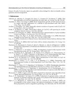
Fig. 8. Power spectrum of transmit signal with spectrum-hole of 6.6%


Fig. 9. Range spectra with and without hole. A point target is placed at 2.2m
3.3 Effect of spectrum-hole
The effect of spectrum-hole on the range spectrum is presented where the measurement
specification is shown in Table 1. Two sphere targets with -9dBsm and -15dBsm are
measured in an RF anechoic chamber (Skolnik, 2001) (Nakamura et al., 2011). The
measurement was conducted in an RF absorber where theses targets on turn table were
placed at 2.2m and 3m from the antenna. Fig.10 shows the range spectrum with spectrum-
hole of 6.6%s, which is compared with that without hole. Please note that the other echoes at
0.8m and 1.6m are from the turn table. Fig.11 shows the range spectrum as a function of
rotation angle where the distane from thsese targets to the antenna are almost equal at the
rotation angle of 90 degree. These targets are found to be discriminated because of the range
resolution of approximately 15cm. The measurements were conducted for
f
Δ
= 34.5MHz
and N=30. Consider
f
Δ
=
7.5MHz and N=133, however, the maximum detectable range d
max

is 20m and the range-resolution is approximately 15cm which is applicable to the short-

range automotive radar.
From the measurement results, it can be concluded that the stepped-FM radar without high
speed A/D devices can be coexistent with other narrowband wireless applications.
Ultra-Wideband Automotive Radar

113
Frequency 3~4GHz
Stepped width Δf 34.5MHz
Number of step N 30
Stepped cycle 10msec
A/D 10kS/sec
IDFT point 1024
Table 1. Measurement specifications


Fig. 10. Range spectra for two targets when the spectrum-holes is 6.6%

Fig. 11. Range spectrum as a function of for two sphere targets
4. Detection using trajectory estimation
Short-range automotive radar with high range-resolution should suffer from clutter because
of its very broad lateral coverage. It is therefore an important issue to detect moving
automobile in heavy clutter conditions. The clutter may be generally classified from
Advances in Vehicular Networking Technologies

114
automobile by the Doppler, but it will be difficult for a very short-pulse of UWB-IR radar.
This is because a shorter pulse will have better range-resolution, but poorer Doppler
resolution. Observing the range profile during several micro-seconds, however, each object
echo’s trajectory is estimated using Hough transformation and the Doppler is then
calculated (Okamoto et al., 2011). When the speed of object is almost constant during the

time, for example, the trajectory is regarded as linear on the time-range coordinate (Hough
space). As a result, moving automobiles are separated from stationary clutter in the Hough
space and detected/tracked with high range. The field measurement results at 24GHz are
presented.
4.1 Time-range profile
Fig.12 shows an example of received range profile on a roadway for a bandwidth of 1GHz.
The profile includes many echoes distinguishable with different delay. Detection,
recognition and tracking of automobile in clutter are very important issues in automotive
radar. Traditionally, the received range profile for each transmit pulse is compared against a
given threshold and a detection decision is made. And once the decision is successfully
done, the range profile is discarded and the next one is considered. This is called threshold
detection. However it is not easy to detect some automobiles simutaneously in heavy clutter
because the automobiles can’t be distinguished from clutter in frequency domain. A time-
range profile based detection is useful for the UWB-IR radar where moving automobiles are
classified from clutter by observing the range profile. Fig.13 shows the range profiles as a
function of transmit pulse number, which is called time-range profile. It is seen from Fig.13
that each echo’s trajectory may be estimated and the Doppler is then calculated.
4.2 Hough transform
Hough transform (HT) has been widely applied for detecting motions in the fields of image
processing and computer vision. Consider the time-range profile as shown in Fig.13, the
time trajectory of each object echo can be estimated by the HT, which is a computationally
efficient algorithm in order to detect the automobile on time-space data map. For example,
the trajectory would be linear for a short duration of 0.1 second or less, thereby the Doppler
can be calculated from the inclination of line.


Fig. 12. Power range profile for a roadway
Ultra-Wideband Automotive Radar

115

Fig. 13. Time-range profiles for 50 nanosecond pulses
4.3 Automobile classification
A. Measurement set-up and procedure
The measurements were conducted on a roadway as shown in Fig.14. The detail
specification is shown in Table 2. The four automobiles were driven along the roadway and
the received signals were processed on board. A pulse repetition interval (PRI) of 15ms is
considered for the scenario of Fig.14. The antennas with a beam-width of 70° in horizontal
direction were placed 60cm above the ground. Please note the anti-collision radar is
designed for short-range/wide-angle object detection.



(a) Measurement scene (b) Measurement scenario
Fig. 14. Measurement scenario
Advances in Vehicular Networking Technologies

116
Bandwidth
5GHz, 1GHz
（centered at 24GHz）
Polarization H-H. plane
Type Double-ridged Horn
Gain
12.5dBi
（24GHz）
Antenna
Height 60cm
Sedan: #1 4.64m×1.72m×1.34m
SUV: #2 4.42m×1.81m×1.69m

Target
Mini-van: #3 4.58m×1.69m×1.85m
Table 2. Measurement parameters
B. Measurement results
Fig.15 shows the flow of HT algorithm from time-range profile to trajectory line. The quasi-
images (8bits time-range image) for BW=300MHz and 500MHz are shown in Fig.15(a) and
(b) respectively. Many trajectories are plotted by the Hough space translation. The number
of trajectory lines depends on the signal-to-clutter ratio (SCR) and the window size to
observe the time-range profile. Some trajectory lines of a time-range profile would be
connected to the lines of the following profile. Therefore the trajectory of object echo can be
selected using the continuity between the consecutive time-range profiles, while the quasi
trajectory should be discarded. Fig.16 (a) shows the estimated trajectory lines for a BW of
500MHz. It is seen that many lines are depicted because of significant clutter. Fig.17(b)
shows the survived lines by the algorithm of Fig.15 where three time-range profiles for 20
pulses are used. It is seen that clutter can be estimated from the Doppler. Fig.18 also shows
the estimated lines for a BW of 300MHz. The results of Figs. 17and 18 are found to agree
with the scenarios. The measurements were also conducted for different scenarios of side-
looking and back-looking radar and the trajectory estimation scheme is found to be useful in
order to classify the automobile from heavy clutter.


Fig. 15. Signal flow for HT algorithm
Ultra-Wideband Automotive Radar

117

(a) BW=500MHz (b) BW=300MHz
Fig. 16. Quasi-images of time-range profile

(a) Estimated trajectory lines by HT (b) Survived trajectory lines
Fig. 17. Estimated trajectory line (BW=500MHz)


Fig. 18. Estimated trajectory line (BW = 300MHz)
5. Target discrimination
Automotive radar is required to detect automobile accurately, but not to detect clutters
falsely, even in complicated traffic conditions. One-dimensional range profile of an
Advances in Vehicular Networking Technologies

118
automobile target has dependence on the shape because it has some remarkable scattered
centers. Therefore the different types of automobile has different range profile feature which
can be used as a unique template for automobile target discrimination/identification purpose
in tracking mode. That is, the target is detected accurately by the correlation of received
signal with template. The scheme also offers real-time operations unlike two-dimensional
image processing (Overiez et al., 2003) (Sato et al., 2006). The measurement results are
presented for various types of automobile (Matsunami et al., 2009) (Matsunami et al., 2010).
5.1 Target discrimaination and identification
Figs.19(a)-(c) show the measured range profile for various bandwidths where a sedan typed
automobile was placed at approximately 10m. Please note that the profiles are expressed as
a function of range-bin corresponding to the range-resolution (=1/BW). Echoes from
various objects are found to be distinguished for wider bandwidth. It is seen that there exist
some remarkable scattered centers. However the feature is not so clear because of
scintillation and noise. Figs.20-22 show range profiles for various bandwidth where the non-
coherent integration of 50 pulses was conducted in order to reduce the scintillation and
noise. For the dedan, some strong echoes are seen from the side mirror and interior, and the
SUV shows a unique feature.

(a) BW=500MHz

(b) BW=1GHz

(c) BW=5GHz
Fig. 19. Power range profiles for various values of BW. A sedan was placed forward the
radar antenna where the antenna to target separation was approximately 10m
Ultra-Wideband Automotive Radar

119

(a) Sedan (b) Mini-van

(c) SUV (d) Mini-truck
Fig. 20. Unique profiles of automobile (BW=5GHz)

(a) Sedan (b) Mini-van

(c) SUV (d) Mini-truck
Fig. 21. Unique profiles of automobile (BW=1GHz)
Advances in Vehicular Networking Technologies

120

(a) Sedan (b) Mini-van


(c) SUV (d) Mini-truck
Fig. 22. Unique profiles of automobile (BW=500MHz)
5.2 Profile matching

Range profiles have been measured for four automobile #1~#4 (sedan, mini-van, SUV and
mini-truck) which have been processed as the template. And the profile matching rate is
calculated for various unknown automobiles. The matching rate is shown in Table.3-5. For
BW=500MHz or more, it is higher than 96% when the automobile is the same as the
template and each automobile can be detected. Assuming a correlation value of 0.6 for the
discrimination, each profile can be identified in clutter since it has unique feature with god
cross-correlation.

Subject vehicle
Template
Sedan Mini-van SUV Mini-truck
Sedan
99.1
22.5 26.9 19.9
Mini-van 13.1
96.9
14.9 15.5
SUV 8.6 4.6
98.6
21.6
Mini-truck 16.8 20.8 15.3
98.2
Table 3. Matching rate [%]（BW=5GHz）
Ultra-Wideband Automotive Radar

121
Subject vehicle
Template
Sedan Mini-van SUV Mini-truck
Sedan

99.4
30.4 53.7 6.2
Mini-van 19.5
96.0
24.8 28.3
SUV 45.1 19.3
99.3
18.4
Mini-truck 14.7 24.8 31.7
98.6
Table 4. Matching rate [%]（BW=1GHz）

Subject vehicle
Template
Sedan Mini-van SUV Mini-truck
Sedan
99.9
38.0 76.6 33.5
Mini-van 38.0
98.9
19.2 31.4
SUV 55.3 25.3
98.2
31.7
Mini-truck 31.2 20.0 33.0
99.3
Table 5. Matching rate [%]（BW=500MHz）
6. Conclusion
UWB-IR short-range radar a5 24/26GHz will be used for various applications such as pre-
crash detection and blind spot surveillance. The short-range radar has a few significant

problems to be overcome such as multiple targets detection and clutter suppression.
This chapter has presented how to detect multiple automobile targets in clutter. The
presented results are as follows;
•
UWB-IR radar requires high speed A/D devices to synchronize and detect the received
nanosecond echo, thereby the system becomes very complicated and expensive. In
section 3, the use of stepped-FM scheme which does not require high speed A/D has
introduced for UWB-IR radar. In addition it offers spectrum hole to coexist with
existing wireless systems.
•
UWB-IR short-range radar is expected to provide a wide coverage in azimuth angle.
Therefore, increased clutter makes it difficult to detect multiple automobile targets.
Section 4 has introduced a multiple target detection scheme in heavy clutter using the
trajectory of radar echoes.
•
Section 5 has introduced a target identification scheme in order to improve the
detection performance where a power delay profile matching is employed and the
usefulness has been demonstrated by the measurement at 24GHz. The results have
showed that automobile targets can be recognized and identified.
7. References
Skolnik, M. (2001). Introduction to Radar systems, 3rd ed., McGraw-Hill, ISBN0-07-288138-0,
New York
Advances in Vehicular Networking Technologies

122
Taylor, J. D. (1995). Introduction to Ultra-wideband Radar Systems, CRC Press LLC, ISBN0-
8493-4440-9, Wsshington, D.C
Matsunami,I.; Nakahata, Y.; Ono, k. & Kajiwara,A. (2008). Empirical Study on Ultra-
wideband Vehicle Radar, Proc. of IEEE Vehicular Technology Conference, ISBN 978-1-
4244-1722-3, 8G-5, Calgary, Sept. 2008.

Nakamura,R.; Yokoyama,R. & Kajiwara,A. (2010), Short-Range Vehicular Radar Using
Stepped-FM Based UWB-IR, Proc. of IEEE Radio and Wireless Symposium, ISBN 978-
1-4244-4726-8, New Orleans, Jan. 2010.
Wehner, D. R. (1995). High-Resolution Radar, Artech House, ISBN978-0-89006-727-7, pp.197-
255, 1995.
Nakamura,R. & Kajiwara,A.(2011), Empirical Study on Spectrum-Hole Characteristics of
Stepped-FM UWB Microwave Sensor, to be appeared in Proc. of IEEE Radio and
Wireless Symposium, Jan. 2011.
Okamoto,Y.; Matsunami,I. & Kajiwara,A.(2011), Moving vehicle discrimination using
Hough, transformation, to be appeared in Proc. of IEEE Radio and Wireless
Symposium, Jan. 2011.
Ovariez,J.P.; Vignaud,L.; Castelli,J.C.; Tria, M., & Benidir,M.(2003). Analysis of SAR image
by multidimensional wavelet transform. IEE Proc. Radar Sonar Navig., pp.234-241,
Aug.2003.
Sato,T. & Sakamoto,T(2006). Reconstruction Algorithms for UWB Pulse Radar Systems,
IEICE Trans. Comm., ISBN1344-4697, vol.J88-B, pp.2311-2325, Dec.2006.
Matsunami,I. & Kajiwara,A.(2009). Power Delay Profile Matching for Vehicular Radar, Proc.
of IEEE Vehicular Technology Conference, ISBN 978-1-4244-2514-3, 5E-1, Anchorage,
Sept. 2009.
7
An Ultra-Wideband (UWB) Ad Hoc Sensor
Network for Real-time Indoor Localization of
Emergency Responders
Anthony Lo
1
, Alexander Yarovoy
1
, Timothy Bauge
2
, Mark Russell

2
,
Dave Harmer
2
and Birgit Kull
3

1
Delft University of Technology,
2
Thales Research & Technology Limited,
3
IMST GmbH,
1
The Netherlands
2
UK
3
Germany
1. Introduction
A localization system is a network of nodes, which is used by an unknown-location node to
determine its physical location. The Global Navigation Satellite System, GNSS (Hofmann-
Wellenhof, 2008) is an example of a widely used outdoor localization system. However,
outdoor localization systems perform poorly in indoor environments due to strong signal
attenuation and reflection by building materials, and no line-of-sight propagation. Thus,
Indoor Localization Systems (ILSs) are needed to provide similar localization inside
buildings. ILSs have many potential applications in the commercial, military and public
safety sectors. This chapter focuses on the public safety application. The considered ILS is
used to track emergency responders, e.g. fire-fighters and policemen, who carry out search
and rescue missions in the disaster zone such as building fires and collapsed tunnels. Such

an ILS was first crystallized in the EUROPCOM (Emergency Ultra wideband RadiO for
Positioning and COMmunications) project (Harmer, 2008; Harmer et al., 2008). The
EUROPCOM system is an ad hoc sensor network which comprises a small number of base
or reference nodes deployed outside surrounding a building, and the rest of the nodes are
unknown-location nodes which are worn and deployed by emergency responders entering
the hostile building. The unknown-location node is self-localized by collectively
determining its position relative to base nodes. Additionally, the unknown-location node is
also allowed to determine its position relative to neighboring unknown-location nodes. This
greatly enhances the accuracy and robustness of the ILS. It is fully autonomous and can be
rapidly deployed with little human intervention.
Ultra-WideBand (UWB) is the radio transmission technology used by the EUROPCOM
system. A UWB signal is defined to be one that possesses an absolute bandwidth of at least
500 MHz or a fractional bandwidth larger than 20% of the center frequency. Currently,
several UWB technologies exist, namely direct sequence UWB, impulse radio UWB, Multi-
Advances in Vehicular Networking Technologies

124
band Orthogonal Frequency Division Multiplexing (MB-OFDM) UWB, Chaotic UWB, and
Frequency Hopping (FH-UWB). The EUROPCOM system selected FH-UWB because it
offers significantly better range and position accuracy than other technologies such as pulse
UWB (Frazer, 2004).
A great deal of effort has been expended on localization algorithms, but the Medium Access
Control (MAC) and routing protocols for ILS have received very little attention yet. Unlike
other ad hoc sensor networks, the considered ILS exhibits unique characteristics. Therefore,
it poses new technical challenges in the MAC and multi-hop routing protocol design. Firstly,
the ILS is heterogeneous in the sense it is composed of different types of nodes with varying
capability, processing power and battery energy. Secondly, the ILS operates in a highly
dynamic and hostile environment. Lastly, emergency applications require fast localization in
the order of seconds. In order to address these challenges, we propose a novel Self-
Organizing Composite MAC (SOC-MAC) protocol and a Lightweight and robust Anycast-

based Routing (LAR) protocol. Cross-layer approach is present in the design to attain highly
optimized, bandwidth- and energy-efficient protocols.
2. Network architecture of an Indoor Localization System (ILS)

CU
BU
DU
MU
MU
Incident Zone
non-UWB link
(Implementation dependent)
UW
B

L
in
k
BU
BU
BU
BU
MU
MU
DU
DU
Legend: BU Base Unit
CU Control Unit
DU Dropped Unit
MU Mobile Unit

Fig. 1. Network Architecture of an Indoor Localization System
The assumed ILS, which is an ad hoc sensor network, consists of four types of nodes: a
Control Unit (CU), Base Units (BUs), Dropped Units (DUs) and Mobile Units (MUs), as
shown in Fig. 1. The MU is a sensor that is worn by every emergency responder. The MU
has the capability to calculate its position which is in turn delivered to the CU. The BUs are
located outside and around the incident area, while maintaining wireless connectivity with
An Ultra-Wideband (UWB) Ad Hoc Sensor Network for
Real-time Indoor Localization of Emergency Responders

125
the emergency responders inside the building. Unlike other units, the position of BUs is
known and most likely to be acquired through GNSS. Furthermore, the BUs will remain
stationary throughout the entire mission. The DUs are strategically placed in the incident
area by emergency responders to serve as relay nodes once the MUs lose wireless
connectivity with the BUs. Similar to MUs, the DUs can determine their positions and relay
them to the CU. The CU provides the main visual display to the rescue coordinators,
showing the current position and direction of movement of individual emergency
responders with respect to the incident area topology, e.g. a building. As shown in Fig. 1,
the ILS is composed of a UWB subnetwork and a non-UWB subnetwork. The reason for two
separate subnetworks is that the CU is not involved in the localization process. Thus, more
radio resources are available for the UWB subnetwork, in particular, when the number of
MUs increases.
2.1 System assumptions
In this subsection, we state several assumptions made in the design of the MAC and routing
protocols. The MAC and routing protocol design assumes the FH-UWB technology is
employed by the Physical layer of the BU, the DU and the MU. The operating bandwidth of
the FH-UWB units is 1.25 GHz which consists of 125 carrier frequencies. This means, the
carrier spacing is 10 MHz. The center frequency is located at 5.1 GHz. Each unit follows a
fixed hop pattern. The pair CU-BU communicates over a non-UWB link. Similarly, the BU-

BU transmission is also over non-UWB links. The rationale for using a non-FH-UWB
technology is that more radio resources are available to the FH-UWB subnetwork. Since the
non-FH-UWB technology is implementation-dependent, we will not further deal with the
specifics of the non-UWB technology in the rest of the chapter. The design of the MAC and
routing protocols is described in subsections 2.2 and 2.3, respectively.
2.2 A Self-organizing Composite Medium Access Control (SOC-MAC) protocol
As each MU is mobile, it will determine and transmit its position information to the CU
periodically. For instance, in order to cope with user mobility in the order of 0.5 m/s
(walking speed), an MU needs to measure and transmit position information to CU at a rate
of one position packet per second. As a result, SOC-MAC is based on the Time Division
Multiple Access (TDMA) because such a MAC is particularly suited to the periodic nature of
localization process. Unlike traditional TDMA, SOC-MAC is designed for ad hoc networks
with no requirement for a central controller for allocating time slots as it is self-organizing.


RA-TDMA
A-TDM AI-TDMA
Reserved TDMA

Fig. 2. SOC-MAC
Advances in Vehicular Networking Technologies

126
Using SOC-MAC, each unit can autonomously select and reserve time slots based only on
local network knowledge without the need of dedicated signaling messages.
As shown in Fig. 2, the SOC-MAC protocol operates in two phases: a Random Access
TDMA (RA-TDMA) phase and a Reserved TDMA phase. The former phase is invoked by a
unit prior to joining the network or when the unit has not used any time slots in the
previous superframe; thus, there are no reservations in the current frame. In this phase, a
unit acquires a time slot through a random access mechanism. Once a time slot has been

acquired, SOC-MAC will enter the Reserved TDMA phase. The RA-TDMA phase and the
Reserved TDMA phase are described in the following subsections.
2.2.1 Random Access TDMA (RA-TDMA) phase
The UWB medium is segmented into SOC-MAC superframes, each of which has a constant
period of T seconds. Each superframe is in turn partitioned into N orthogonal time slots of
duration T/N seconds. The start of the superframe is provided by one of the BUs, known as
the Master BU (MBU). Naturally, MBU will occupy the first time slot. Units unable to hear
the transmissions of MBU will synchronize to the TDMA frame by monitoring the
transmissions of other neighboring units, which will identify the time slot in which they are
transmitting. From this time slot number information, the start of the frame can be inferred.
Fig. 3 depicts the structure of the superframe and time slot. Each time slot can be used for
either data transmission (referred to as “data slot”) or ranging (referred to as “ranging slot”).
The latter time slot format is specifically used for determining the range between two units.
Thus, the ranging slot can accommodate a very limited payload. The MAC header includes
identifiers of up to five ranging units, denoted as “R1 ID” to “R5 ID”, which have been
selected to respond to ranging requests. The final part of the ranging slot is reserved for the
corresponding “pong” responses from “R1 ID” up to “R5 ID”. Unlike ranging-slot, data-slot
is purely utilized to transmit user data and can accommodate larger payload. The MAC
header of the two slot structures contains similar fields except the ranging-slot includes the
ranging unit identifiers and the position data of the transmitting unit (i.e., TX ID POS).
Hence, the MAC header of the ranging-slot is longer and has to be split into two parts
separated by two pilot tones as shown in Fig. 3.
In general a unit enters the RA-TDMA phase prior to joining the network. Fig. 4 contains the
flow chart of the RA-TDMA phase. Before the unit can transmit in a time slot, it must listen
to the physical channel for at least one complete TDMA superframe period. During this
period, the unit constructs a list of one-hop neighbors and a map of their time-slot usage.
Based on the time-slot usage map, the unit derives a list of vacant time slots in the
forthcoming superframe. The number of vacant slots in the list is denoted as candidate slot
counter (csc) in Fig. 4. When a first vacant time slot in the next superframe arrives, the p-
persistent algorithm is applied to determine if this vacant time slot can be used for

transmission. The p-persistent algorithm defines two parameters, namely P1 and P2. P2 is
inversely proportional to csc, and P1 is randomly selected from an interval [0 1]. If P1 is
equal to, or less than P2, then the vacant time slot is reserved and transmission should occur
in the reserved time slot. If not, the number of vacant time slots csc in the list is decremented
by one and the same procedure is repeated for the next vacant time slot. The p-persistent
algorithm minimizes the chance that two or more units in the RA-TDMA phase are
contending for the same time slot. A low csc increases the probability of selecting the next
vacant time slot. The number of unsuccessful attempts in reserving a time slot is recorded in
attempt count (ac). Once a vacant time slot has been successfully reserved, the RA-TDMA
phase ends and the reserved TDMA phase sets in to complete the channel access procedure.
An Ultra-Wideband (UWB) Ad Hoc Sensor Network for
Real-time Indoor Localization of Emergency Responders

127

0 1 2 3 4 5 6 N 0 1 2 3 4 5 6 N
Pilot Pilot
MAC
Header
(Part I)
Pilot Pilot R0 R1 R2 R3 R4 R5
Responses of 5 UnitsData from Transmitting Unit
MAC Header
(Part II)
and Payload
Superfr ame 0
T
Superframe 1
T
Pilot Pilot

MAC
Header
Pilot Pilot Pilot PilotNWK Payload
Ranging-Slot Format
Data-Slot Format
FEC
Rate
MLEN SYNC
TX
ID
R0
ID
R2
ID
R1
ID
R4
ID
R3
ID
MAC
Info
(I)
CRC
FEC
Rate
MAC
Info
(II)
NWK

Payload
CRC
TX ID
POS
RX
ID
MAC
Reserved
ST
Msg
Type
Submsg
FEC
Rate
MLEN SYNC
TX
ID
Bit Sequence for identifying
Data Slot
MAC
Info
CRC
ST
Msg
Type
Submsg
(*)
RX
ID
MAC

Reserved
SLOTNUM Unused
SOFF Unused
SOFF LEN
(*) Thi s field has the sam e structur e as the “submsg” field in the R anging Slot
(+) This field has the same structure as the NWK Header in the Rangi ng Slot
or
or
(Submessage Type 1)
(Submessage Type 2)
(Submessage Type 3)
For A - TDM A w hen ST > 0
For A-TDMA when ST = 0
For I- TDM A to reserve extr a tim e slots
NWK
Header
NWK
Header
(+)
Hop
Count
Congestion
Level
Reserved

Fig. 3. SOC-MAC Superframe
Advances in Vehicular Networking Technologies

128

Is slot vacant
?
Analyze next slot in
forthcoming superframe
Select random
number , p1, from [0,1]
P1 ≤ P2
?
A slot is selected ;
RA -TDMA phase ends ;
Reserved TDMA phase starts ;
ac = 0;
ac = ac + 1 ;
csc = csc – 1;
P2 = 1/csc;
Yes
Yes
No
No
Start
csc = number of
vacant slots ;
P2 = 1/csc;
ac = 0;
End
Scan one com pl ete
superframe

Fig. 4. Flow Chart of RA-TDMA
2.2.2 Reserved TDMA phase

The Reserved TDMA mode comprises two operations, namely the Autonomous TDMA (A-
TDMA) and the Incremental TDMA (I-TDMA). The latter is used to acquire additional slots
in the same superframe in addition to the one acquired in the RA-TDMA phase. A-TDMA is
responsible for managing the acquired time slots.
A-TDMA
Once a slot has been acquired through RA-TDMA and/or I-TDMA, the same time slot is
automatically reserved for the next Slot_Timeout (ST) superframes, where ST is randomly
picked from an interval [1 MAX_TIMEOUT]; MAX_TIMEOUT is a MAC design parameter.
A-TDMA is responsible for keeping ST up-to-date. That is, ST is decremented by one in each
new superframe. ST is included in the MAC header so that other units can determine when the
time slot will be free. When ST > 0, the Submessage Type 1 is used, which contains the time-slot
number (SLOTNUM) of the currently reserved time slot as illustrated in Fig. 3. When a time
slot expires (i.e., ST = 0), A-TDMA randomly chooses a vacant time slot in the next superframe
from a list of vacant time slots in the time-slot usage map, and pre-announces to the other
An Ultra-Wideband (UWB) Ad Hoc Sensor Network for
Real-time Indoor Localization of Emergency Responders

129
units the offset between the present time slot and the newly selected time slot (SOFF
expressed in number of time slots) using the format Submessage Type 2 in the current
superframe as shown in Fig. 3. This allows other units to find this unit in the next superframe
without searching and to update the time-slot usage map. The new time slot will only be used
in the next superframe. The continuous change of time-slot positions ensures that if two or
more units had chosen the same time slot in the RA-TDMA phase, the collision can only
persist for a maximum of MAX_Timeout superframes before one or all involved units must
choose a different time slot. Thus, the collision is resolved through a probabilistic means.
Hence, MAX_TIMEOUT must be small in order to reduce the number of collisions that are
energy-wasting. On the other hand, if MAX_TIMEOUT is too small then neighbor units need
to perform frequent updates on the time-slot usage map, which in turn increases power
consumption. The new time slot is assigned a new ST value which is obtained using the same

process as described above. The A-TDMA algorithm is depicted in Fig. 5.


Is
Slot_ Timeout
Expired ?
Check Slot _Timeout
Select a r andom
slot from a set of vacant sl ots
Yes
No
Pre -announce selected slot in
Current superframe
Start
End

Fig. 5. Reserved TDMA Phase: ATDMA Operation
I-TDMA
The time slot acquired during the RA-TDMA phase is the first and only one for each unit. If
a unit needs extra time slots, then I-TDMA is employed to reserve the extra time slots in the
same superframe to increase the data rates. I-TDMA calculates the number of required time
slots N
I
based on the actual queue length provided by the Network layer. It searches for a
block of N
I
successive vacant time slots in the time-slot usage map. If not available, N
I
is
reduced until the search is successful. The number of reserved time slots (LEN) and the

offset (SOFF) between the current and the first new time slot are advertised using the format
Submessage Type 3, refer to Fig. 3, so that all other units are informed about the new
reservations. In principle each new time slot can be used for another I-TDMA operation so
that the number of time-slot reservations can grow more rapidly. Hence, the usage of I-
TDMA needs to be restricted if the channel is busy and the number of vacant time slots is
small. Note that in almost all cases the A-TDMA operation is required, while the I-TDMA
Advances in Vehicular Networking Technologies

130
operation is only sporadically needed to increase the data rates by reserving additional time
slots. In order to free reserved time slots, the time slots are simply not renewed by A-TDMA
after Slot_Timeout superframes.
2.3 A Lightweight and Robust Anycast-based Routing (LAR) protocol
The Lightweight and Robust Anycast-based Routing (LAR) protocol routes data packets
from MUs or DUs to the nearest BU. There is no exact destination BU for a data packet.
Thus, routing decisions must rely on routing parameters and packet types. LAR defines two
routing parameters, namely hop count and congestion level. Hop count indicates the distance
of a unit (in terms of the number of hops) to a reference BU. It increases monotonically at
each hop. Congestion level is used to indicate the buffer occupancy of a unit. These routing
parameters are not disseminated using dedicated routing packets but carried and
propagated in the Network (NWK) header of data packets. Thus, LAR does not incur
routing packet overheads. The format of the NWK header is depicted in Fig. 3. This means
that irrespective of the data type, the NWK header always contains the mandatory routing
parameters. The NWK header occupies 12 bits in a total of 1831 bits in one time slot of the
SOC-MAC superframe. Therefore, the overheads of the NWK header for routing are less
than 1%, which conserves bandwidth and energy.
Route establishment is initiated by BUs to form spanning trees rooted at each BU. This is a
natural choice because each BU periodically broadcasts its position which is known
beforehand, while DUs and MUs just listen to the BU broadcasts since they need to
determine their position. The BU sets the initial value for the hop count and congestion

level. From the BU broadcasts, the DUs/MUs create a new entry in the routing table if it
does not exist. The routing table entry contains the following fields: neighbor unit id, hop
count, congestion level, FEC level and the expiration time of the entry. The first field identifies the
address of the unit that broadcasts the data packet, which represent the next-hop unit for the
route towards a destination BU. The neighbor unit id is contained in the MAC header. Note
that the unit maintains only the next-hop routing state, which provides the routing protocol
with a high degree of scalability. The hop count in the routing table is incremented by one
with respect to the received hop count. For instance, if the incremented hop count is n+1
then the unit is n+1 hops away from the destination BU. The congestion level field is
extracted from the NWK header. FEC (Forward Error Correction) level determines the
channel bit rate for communicating with the next hop of the neighbor unit id. Four FEC
levels, viz., FEC-1 to FEC-4, are defined. FEC-4 provides the highest bit rate but no or the
lowest level of error protection. The FEC level is also contained in the MAC header. Once a
DU/MU has determined its position, it can broadcast its position. The hop count in the
NWK header is obtained from the selected route in the routing table entry, while the
congestion is set to the maximum of its congestion level and that in the routing table entry.
In the case of multiple entries in the routing table, a route selection algorithm with load
balancing is used to choose the next hop. The algorithm will be described in subsection 2.3.1.
So far, we have focused on route construction from an MU/DU to a destination BU, which is
referred to as forward route. A reverse route (from a BU to an MU or DU) can be
constructed using data packets sent on the forward route. One such data packet is position
reporting which is used to transport position data to the BU. Position reporting packets are
periodically sent by an MU and DU. The position reporting packets are transmitted using a
forward route selected by the unit to a destination BU. All units along the forward route
store the source and forwarding unit identifiers in their routing table. The latter identifier is
An Ultra-Wideband (UWB) Ad Hoc Sensor Network for
Real-time Indoor Localization of Emergency Responders

131
the address of the intermediate unit that forwards the data packet while the source identifier

is the address of the unit which generates the position reporting packets. No other routing
parameters are needed for the reverse route. Since the position broadcasting and position
reporting are periodic, the forward and reverse routes are always up-to-date. Therefore, no
specific route recovery or maintenance functions are required.
2.3.1 Load balancing
Load balancing is achieved using the congestion level parameter, which is based on the
occupancy of queues in a unit. The queues allocated by a unit are assumed to be fixed size.
The congestion level is then deduced from the queue occupancy as shown in Table 1.

Congestion Level Queue Occupancy Definition
0 - 2 20% - 40% full Not congested
3 - 4 50% - 60% full Slightly congested
5 - 6 70% - 80% full Congested
7 90% full Heavily congested
Table 1. Congestion Levels for Load Balancing
2.3.2 Route selection


next-hop candidate
Is candidate hop
count smallest ?
next -hop candidates with
smallest hop count
Is candidate
Congestion level
lowest?
Advertised selected
next hop
No
Yes

No
Yes
Yes
Start
End

Fig. 6. Next-hop Selection Algorithm with Load Balancing
Advances in Vehicular Networking Technologies

132
Hop count is the primary routing metric, while congestion is the secondary metric due to the
delay at the MAC layer, which cannot be tolerated by real-time data packets. In the case of
multiple entries in the routing table, LAR must select the candidate route with the smallest
hop count. If there are several candidate routes with the same hop count then the candidate
with the lowest congestion level is picked. By selecting the candidate route with the smallest
hop count the selection algorithm can guarantee loop-free delivery as a data packet is
always forwarded from a unit with a higher hop count to a unit with lower hop count. The
selection algorithm is shown in Fig. 6.
3. Simulation set-up
The feasibility and performance of SOC-MAC and LAR are evaluated by means of
simulation. To this end, we extended the Mobility Framework (MF) (Mobility Framework)
module by incorporating a model for a UWB Physical layer, the SOC-MAC protocol, the LAR
protocol and the Application layer, and the ILS network entities. MF is an add-on package for
simulating mobile and wireless networks on the OMNeT++ platform (OMNeT++) which is a
powerful generic, object-oriented and discrete-event simulation tool. Naturally, MF can be
easily extended for simulating the ILS network. Thus, three new simulation nodes, namely
BUhost, DUhost, and MUhost, were defined. These nodes correspond to the units BU, DU
and MU, respectively. CU was not modeled because it is in the non-UWB subnetwork which
is implementation-specific. Fig. 7 depicts a sample of the simulation network, which consists
of four BUhosts, two DUhosts and four MUhosts. In each of the simulation nodes, three

protocol models, viz., the application, the network and the Network Interface Card (NIC)
were defined as extensions to the corresponding models in MF. The internal structure of the
node is shown in Fig. 8(a). The Blackboard and Mobility models were used without
extensions. Note that BUhost, DUhost and MUhost have the same internal node structure.
The application model,
EuropAppLayer, the network model, EuropNetwLayer, the MAC model,
EuropMacLayer, and the Physical model are described in the next subsections.


Fig. 7. Simulation Network
An Ultra-Wideband (UWB) Ad Hoc Sensor Network for
Real-time Indoor Localization of Emergency Responders

133

EuropAppLayer
EuropNetwLayer
EuropNIC
BU/DU/MUhost
Blackboard
Mobility
EuropMacLayer
SnrDecider
EuropSnrEval
NIC
(a) (b)

Fig. 8. Node and NIC Structure
3.1 Physical layer model
The Physical model is divided into EuropSnrEval and SnrDecider as shown in Fig. 8(b). The

former was extended from SnrEval in MF while the latter was used as it is. EuropSnrEval is
used to calculate the Signal-to-Interference-plus-Noise (SINR) of a received MAC frame. The
SINR is defined as

,max
10log
r
n
P
SINR
PI
=
+
(1)
where P
r,max
is the strongest received signal power among the received signals, based on the
capture effect (Rappaport, 2001). P
n
is the Additive White Gaussian Noise (AWGN). I is the
interference power which is defined as the sum of all received signal power excluding P
r, max
.
The interference power I is expressed as

,maxr
r
P
IP
≠

=
∑
(2)
In case of collision-free transmission, the term I is null. Hence, Equation (1) is reduced to

,max
10log
r
n
P
SINR
P
=
(3)
The computed SINR is passed to SnrDecider which determines whether the MAC frame is
correctly received or not. A MAC frame is considered to be correctly received, if SINR ≥
SINR
th
, where SINR
th
is the SINR threshold. A correctly received frame is delivered to the
EuropMacLayer, otherwise it is discarded. SINR
th
was obtained through physical layer
simulation, which produces Bit Error Rate (BER) plots as a function of SINR. Given a target
BER, SINR
th
is deduced. The physical layer simulation was carried out separately using
another tool since OMNeT++ and MF lack the support for simulating physical layer
functions such as frequency hopping, channel coding, modulation, and signal processing.

Advances in Vehicular Networking Technologies

134
The received power P
r
in Equation (1) is characterized by large-scale fading and small-scale
fading. Large-scale fading represents the average signal power attenuation when
transmitted through the medium. The attenuation or commonly known as Path Loss (PL) as
a function of distance is expressed as (Rappaport, 2001).

/10
00
0
() ( )( ) ,
10
x
d
PL d PL d d d
d
σ
γ
=
≥ (4)
where d
0
is the reference distance, γ is referred to the path loss exponent, and X
σ
denotes the
log-normal shadowing effect with a zero-mean normal distribution (in dB) and standard
deviation σ (also in dB). PL(d

0
) is evaluated using the free-space path loss equation or by
conducting measurements. In our work, PL(d
0
) was determined using the free-space path
loss equation which is given by (Rappaport, 2001)

2
0
0
4
()
c
fd
PL d
c
π
⎛⎞
=
⎜⎟
⎝⎠
(5)
where
max min
.
2
c
f
ff
=

+
f
min
and f
max
are the lower and upper boundary of UWB transmission
frequency band, respectively. Substituting Equation (5) into Equation (4), and let d
0
= 1 m in
our case, we can rewrite Equation (4) as

2
/10
0
4
() 10 ,
x
c
f
PL d d d d
c
σ
γ
π
⎛⎞
=
≥
⎜⎟
⎝⎠
(6)

Small-scale fading represents the wide variations in received signal strength caused by
interference between two or more versions of the transmitted signal arriving at the receiver
at slightly different times. It is typically modeled by the Ricean distribution or the Rayleigh
distribution when there is a line-of-sight or non-line-of-sight, respectively. In UWB systems,
the signal power variations due to small-scale fading are not severe due to the ultra-large
bandwidth of UWB signals and diversity techniques used in the physical layer. Thus, in our
physical channel model, we are only concerned with the large-scale fading. Hence, the
received power P
r,max
in Equation (1) and P
r
in Equation (2) can be calculated using

()
t
r
P
P
PL d
= (7)
where PL(d) is given in Equation (6), and P
t
is the transmit power.
3.2 MAC layer model
The MAC model, EuropMacLayer, captures the complete functionality of SOC-MAC
described in Section 2.2. It was derived from the BasicMacLayer model of MF. The model
definition consists of three parts, referred to as a EuropMacLayer module definition, a
EuropMacLayer protocol data unit definition, and a EuropMacLayer module
implementation. The EuropMacLayer module definition, which is specified using the
OMNeT++ NED language. The EuropMacLayer protocol data unit definition, called

EuropMacPkt, was derived from the MacPkt definition of MF. The derived module contains
An Ultra-Wideband (UWB) Ad Hoc Sensor Network for
Real-time Indoor Localization of Emergency Responders

135
the fields of the EuropMacLayer protocol data unit only. The EuropMacLayer module
implementation contains the algorithms of the composite MAC. Unlike the EuropMacLayer
module definition and EuropMacPkt definition, this module was directly written in the C++
programming language. The EuropMacLayer module definition and EuropMacPkt are
translated into C++ code when an executable of the simulation program is built.
3.3 Network layer model
The Network model, EuropNetwLayer, implements the LAR protocol described in Section
2.3. It was derived from the SimpleNetwLayer model of MF. Similar to the MAC model, it
consists of three parts: a EuropNetwLayer module definition, a EuropNetwLayer protocol
data unit definition, and a EuropNetwLayer module implementation. The EuropNetwLayer
protocol data unit definition, called EuropNetwPkt, was derived from the NetwPkt
definition of MF.
3.4 Application layer model
The application traffic model generates dummy position packets of fixed size at regular
intervals. The dummy position packets carry no real position information and the simulated
nodes do not perform position estimation. This does not affect the performance of SOC-
MAC and LAR as long as the application model can mimic the traffic behavior of the real
system. The application traffic model, called EuropApplLayer, which was derived from
BasicApplLayer of MF. The application traffic model also consists of three parts: a
EuropApplLayer module definition, a EuropApplLayer protocol data unit definition, and a
EuropApplLayer module definition.
4. Simulation results
4.1 SOC-MAC performance
We analyze the performance of SOC-MAC. The performance measures for SOC-MAC are
the successful SOC-MAC packet reception rate and the network throughput. An SOC-MAC

packet consists of a header and payload for both the data- and ranging-slot as illustrated in
Fig. 3. Thus, in one time slot, only one SOC-MAC packet is transmitted. The successful
packet reception rate P in the network is defined as the total number of SOC-MAC packets
received by all units divided by the total number of SOC-MAC packets transmitted by all
units in the network. Hence, P is expressed as

1
1
(1)()
M
i
i
M
j
j
r
P
M
b
=
=
∑
=
−
∑
(8)
where r
i
is the number of MAC packets received by the ith unit, and b
j

is the total number of
MAC packets transmitted by the jth unit. M is the total number of units in the network. The
scale factor in the denominator of Equation (8) is due to the fact that a packet transmitted by
jth unit is received by all the other M – 1 units in the single hop case. Therefore, P is unity in
an ideal case.
Network throughput is defined as the total throughputs of all units, where the throughput
of a unit is the amount of successfully received MAC frames in bits per second. The network