Artificial Neural Networks Industrial and Control Engineering Applications Part 6 potx

Artificial Neural Networks - Industrial and Control Engineering Applications

164
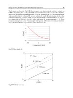
instance in a steel with a carbon content of 0.15wt%, addition of 0.025% Nb increases tensile
strength by 150 MPa.


Fig. 7. Carbon concentration effect in combination with (a) Silicon (b) Manganese (c) Niobium.
Application of Bayesian Neural Networks to
Predict Strength and Grain Size of Hot Strip Low Carbon Steels

165
Figure 8a, displays the effect of strip thickness versus manganese content on the final tensile
strength. The results indicate a drop in tensile strength when final thickness is increased.
This can be attributed to lower cooling rate of thicker strips. Therefore, coarsening takes
place and the tensile strength decreases (Singh et al., 1998). This figure also illustrates the
more influential effects of manganese on thinner strips. Figure 8b reveals the significance of
finishing temperature verses the carbon concentration on tensile strength. It shows that by
decreasing finishing temperature, the final tensile strength increases. Inter-pass
recrystallization and grain growth prevention my causes this effect (Preloscan et al., 2002).
The influence of temperatures on tensile strength is not significant when compared with that
of chemical composition (in specified ranges) (Botlani-Esfahani et al., 2009b).


Fig. 8. Interaction of processing feature (a) Final thickness and manganese concentration, (b)
Finishing temperature and carbon concentration.
Artificial Neural Networks - Industrial and Control Engineering Applications

166
3.4 Grain size model results
The result of this analysis indicates the importance of Si, Mn and C contents on grain

refinement which is significantly greater than the concentration of other elements. The most
effective element for grain refinement is recognized to be that of vanadium. However, its
concentration in these steels is very low. For testing, the results of the model are depicted
when the concentrations of elements are on their mean values which mentioned in Table 2
and the microalloying elements (i.e. Nb, Ti and V) are not present. Figure 9 shows the model
result of this analysis. Manganese stabilizes austenite, therefore decreases austenite to ferrite
transformation temperature and hence refines the grain structure. In addition, manganese


Fig. 9. Model result in respect of silicon and manganese concentration in 0.015 wt %C and
0.035 wt%Al. (a) Absence micro-alloying elements. (b) Minor addition of vanadium (0.008
wt %).
Application of Bayesian Neural Networks to
Predict Strength and Grain Size of Hot Strip Low Carbon Steels

167
can enhance the precipitation strengthening of vanadium microalloyed steels and to a lesser
extent, niobium microalloyed steels (keytosteel). Figure 9a reveals determining role of
silicon on grain size in the absence of microalloying elements (i.e. Nb, Ti and V). The figure
shows that silicon concentration divides the figure into three regions include finer, mild and
coarser grain structures. This figure also indicates that increasing Si content, increases grain
size. This is because silicon is a ferrite stabilizer and promotes ferrite grain growth
(Umemoto et al., 2001). Figure 9b shows that addition of small amount of vanadium
(0.008wt %) to steel severely contracts the coarser grain region. Vanadium acts as a
scavenger for oxides, and forms nano-scale inter-phase precipitations. This is mainly due to
the rapid rate of austenite to ferrite transformation which produces these nano-scale
precipitates (Bhadeshia & Honeycombe, 2006). Furthermore, addition of vanadium also
reduces the finer grain area somewhat. This is because, vanadium is strong carbide former
and the majority of such elements is ferrite stabilizer and therefore, promotes ferrite grain
growth (Zhang & Ren, 2003). The net effect of this minor vanadium addition is to decrease

the sensitivity of grain size to silicon content, and also reduction of coarse grain area.
4. Conclusions
1. The effects of chemical composition and process variables on the tensile strength of hot
strip mill products were modeled by Artificial Neural Network (ANN) moreover a
Bayesian ANN model assisted by RJMCMC is capable of predicting the grain size of hot
strip low carbon steels and can be used as a function of steel composition. The results of
both models are shown to be consistent with experimental data (acquired from
Mobarakeh Steel Company data).
2.
The relative importance of each input variable was evaluated by sensitivity analysis for
tensile strength. The influence of chemical composition on final tensile strength is much
more pronounced than process parameters. Furthermore, grain size model recognizes
the effects of relevant elements in grain refining. These are manganese, silicon and
vanadium. Silicon concentration shows determining role this effect have not reported in
the literature and vanadium reveals great impact on grain refining phenomena.
3.
The results show the effects of the parameters are too complex to model with a simple
linear regression technique. The developed ANN models can be used as guide to
control the final mechanical properties of commercial carbon steel products. The major
advantage of these methods is selection of useful inputs in complex problems with
many inputs. Because many problems in materials science and engineering are similar,
this method is useful for solving them.
5. References
Bhadeshia. H.K.D.H., Honeycombe. R.W.K. (2006) Steels Microstructure and Properties.
3rd ed., Elsevier, London, U.K, 57.
Bhadeshia. H.K.D.H., Lordand. M. Svensson. L.E. (2003) Silicon–Rich Bainitic Steel Welds
Proc. of Int. Conf.: Joining & Welding Solutions to Industrial Problems, JWRI,
Osaka University, Japan, 43-52.
Botlani-Esfahani. M, M. R. Toroghinejad and Key Yeganeh. A. R. (2009a) Modeling the Yield
Strength of Hot Strip Low Carbon Steels by Artificial Neural Network. Materials

and Design 30:9, 3653-3658
Artificial Neural Networks - Industrial and Control Engineering Applications

168
Botlani-Esfahani. M, Toroghinejad. M. R. and Abbasi. Sh. (2009b) Artificial Neural Network
Modeling the Tensile Strength of Hot Strip Mill Products. ISIJ International 49:10,
1583-1587
Doan. C. D. and Yuiliong. S. (2004) Generalization for Multilayer Neural Network Bayesian
Regularization or Early Stopping. Proc. of Asia Pacific Association of Hydrology
and Water Resources 2nd Conference, APHW, Singapore, 1
Gonzalez. JEG. (2002) Study of the effect of hot rolling processing parameters on the
variability of HSLA steels, Master thesis, University of Pittsburgh, USA
Hulka. K. (2003): Niobium Information, 17/98,
Keytosteel.com. Control of high strength low alloy (HSLA) steel properties. www.
keytosteel.com
Lampinen. J. and Vehtari. A. (2001) Bayesian techniques for neural networks - review and
case studies. In K. Wang, J Grundespenkis, and A. Yerofeyev, editors, Applied
Computational Intelligence to Engineering and Business, 7-15.
MacKay DJC. (1992) A practical Bayesian framework for back-propagation networks. Neural
Computation. 4, 415-47.
MathWorks,Inc. />doc/nnet/nnet.pdf, Nat-ick, MA, USA
MEYER, L (2001). History of Niobium as a microalloying element.” In: Proceedings of the
International Symposium Niobium 2001. Niobium Science and Technology.
Niobium 2001 Ltd. Bridgeville: Pa, USA. 359-377
Preloscan. A., Vodopivec. F., Mamuzic. I. (2002) Fine-Grained Structural Steel with
Controlled Hot Rolling. Materiali in Tehnologije, 36, 181.
Parker. S.V. (1997) Modeling phase transformation in hot-rolling steels. PhD Thesis,
University of Cambridge, UK
Ryu. J. (2008). Model for mechanical properties of hot-rolled steels, Master thesis, Pohang
University of Science and Technology, Korea

Singh. S. B., Bhadeshia. H. K. D. H, MacKay. D. J. C., Carey. H, and Martin. I. (1998) Neural
Network Analysis of Steel Plate Processing. Ironmaking Steelmaking, 25, 355.
Umemoto. M., Liu. Z.G., Masuyama. K., Tsuchiya. K. (2001): Influence of Alloy Additions on
Production and Propeties of Bulk Centite. Scripta. Materialia., 45, 39.
Zhang. Y. B., Ren. D.Y. (2003) Distribution of strong carbide forming elements in hard facing
weld metal. Materials. Science and Technology., 19:8. 1029-103.
Vehtari. A., and Lampinen. J. (2002), Bayesian model assessment and comparison using
cross-validation predictive densities, Neural Computation, 14, 2439.
Xu. M., Zeng. G., Xu. X., Huang. G., Jiang. R. and Sun. W. (2006) Application of Bayesian
Regularized BP Neural Network Model for Trend Analysis, Acidity and Chemical
Composition of Precipitation in North Carolina. Water, Air, and Soil Pollution, 172,
167.
8
Adaptive Neuro-Fuzzy Inference
System Prediction of Calorific Value
Based on the Analysis of U.S. Coals
F. Rafezi, E. Jorjani and Sh. Karimi
Science and Research Branch, Islamic Azad
University, Tehran
Iran
1. Introduction
Coal is a chemically and physically heterogeneous and combustible substance that consists
of both organic and inorganic compounds. It currently is a major energy source worldwide,
especially among many developing countries, and will continue to be so for many years
(Miller, 2005).The chemical analysis of coal includes proximate and ultimate analyses. The
proximate analysis gives the relative amounts of moisture, volatile matter, and ash, as well
as the fixed carbon content of the coal. The ultimate or elemental analysis gives the amounts
of carbon, hydrogen, nitrogen, sulfur, and oxygen in the coal (Miller, 2005).
The measure of the amount of energy that a given quantity of coal will produce when
burned is kown as calorific value or heating value. Heating value is a rank parameter and a

complex function of the elemental composition of the coal, but it is also dependent on the
maceral and mineral composition (Hower and Eble, 1996). It can be determined
experimentally using a calorimeter.
Many equations have been developed for the estimation of gross calorific value (GCV)
based on proximate analysis and/or ultimate analysis (Mason and Gandhi, 1983; Mesroghli
et al., 2009; Given et al., 1986; Parikh et al., 2005; Custer, 1951; Spooner, 1951; Mazumdar,
1954; Channiwala and Parikh, 2002; Majumder et al., 2008).
Regression analyses and data for 775 U.S. coal samples (with less than 30% dry ash) were
used by Mason and Gandhi (1983) to develop an empirical equation that estimates the
calorific value (CV) of coal based on its C, H, S, and ash contents (all on dry basis). Their
empirical equation, expressed in SI units, is:
CV = 0.472C + 1.48H + 0.193S + 0.107A – 12.29 (MJ/kg) (1)
Given et al. (1986) developed an equation to calculate the calorific value of U.S. coals from
their elemental composition; expressed in SI units, their equation is:
CV = 0.3278C + 1.419H + 0.09257S – 0.1379O + 0.637 (MJ/Kg) (2)
Neural networks, as a new mathematical method, have been used extensively in research
areas related to industrial processes (Zhenyu and Yongmo, 1996; Jorjani et al., 2007; Specht,
Artificial Neural Networks - Industrial and Control Engineering Applications

170
1991; Chen et al., 1991; Wasserman, 1993; Chehreh Chelgani et al., 2008; Hansen and
Meservy, 1996; Patel et al., 2007; Mesroghli et al., 2009; Bagherieh et al., 2008; Jorjani et al.,
2008; Chehreh Chelgani et al., 2010; Khandelwal and Singh, 2010 ; Sahu et al., 2010;
Yao et al., 2005; Patel et al., 2007; Salehfar and Benson, 1998; Wu et al., 2008; Karacan,
2007).
Patel et al. (2007) predicted the GCV of coal utilizing 79 sets of data using neural network
analyses based on proximate analysis, ultimate analysis, and the density of helium. They
found that the input set of moisture, ash, volatile matter, fixed carbon, carbon, hydrogen,
sulfur, and nitrogen yielded the best prediction and generalization accuracy.
Mesroghli et al. (2009) investigated the relationships of ultimate analysis and proximate

analysis with GCV of U.S. coal samples by regression analysis and artificial neural network
methods. The input set of C, H
exclusive of moisture
(H
ex)
, N, O
exclusive of moisture
(O
ex
), S, moisture,
and ash was found to be the best predictor.
The adaptive neuro-fuzzy inference system (ANFIS), which consists of both artificial neural
networks and fuzzy logic, has been used widely in research areas related to industrial
processes (Boyacioglu and Avci, 2010; Esen and Inalli, 2010; Soltani et al., 2010; Pena et al.,
2010; Chong-lin et al., 2009).
The aim of the present work is to assess the properties of 4540 samples of U.S. coal from 25
states with reference to the GCV and possible variations with respect to ultimate and
proximate analyses using multi-variable regression, the SPSS software package, and the
ANFIS, MATLAB software package.
This work is an attempt to answer the following important questions:
a. Is it possible to generate precise linear or non-linear equations between ultimate and
proximate analysis parameters and GCV for different U.S. coal samples that have a
wide range of calorific values from 4.82 to 34.85 MJ/kg?
b. Is ANFIS a better tool than regression analysis for improving accuracy and decreasing
errors in the estimation of the calorific value of coal?
c. Is it possible to improve the accuracy of predictions by changing “total hydrogen and
oxygen in coal (H and O)” to “H
ex
, O
ex

, and moisture?”
This work is different from previously published work because it involves the first use of
ANFIS to predict the GCV of coal.
2. Experimental data
The data that were used to examine the proposed approaches were obtained from the U.S.
Geological Survey Coal Quality (COALQUAL) database, open file report 97-134 (Bragg et
al., 2009). Samples with more than 50% ash and samples that had a proximate analysis
and/or an ultimate analysis different from 100% were excluded from the database.
Analysis results for a total of 4540 coal samples were used.
The sampling procedures and chemical analytical methods are available at the following
website: The number
of samples and the range of GCV for different states are shown in Table 1.
Table 2 shows the ranges of input variables, i.e., C, H, H
ex
, N, O, O
ex
, total sulfur, ash,
moisture, and volatile matter, that were used in predicting GCV.
Adaptive Neuro-Fuzzy Inference System Prediction
of Calorific Value Based on the Analysis of U.S. Coals

171
State Number of samples Range of GCV (MJ/kg)
Alabama 679 6.05-34.80
Alaska 51 8.65-27.42
Arizona 10 18.54-24.36
Arkansas 52 5.57-34.68
Colorado 172 7.24-33.81
Georgia 25 24.03-34.85
Indiana 101 19.23-28.96

Iowa 73 16.03-26.59
Kansas 19 20.87-28.86
Kentucky 720 18.68-34.03
Maryland 40 23.04-33.48
Missouri 68 23.83-28.63
Montana 140 5.55-20.63
New Mexico 114 8.81-32.15
North Dakota 124 4.85-13.61
Ohio 398 16.43-31.14
Oklahoma 25 23.89-33.31
Pennsylvania 498 13.58-33.10
Tennessee 42 24.61-33.48
Texas 33 9.54-27.74
Utah 103 4.82-30.14
Virginia 368 19.49-34.80
Washington 10 13.14-27.45
West Virginia 340 14.29-34.75
Wyoming 335 6.27-34.23
Table 1. Number of samples and range of GCV (as-received) for different U.S. states

Variable (%) Minimum Maximum Mean Std. Deviation
Moisture 0.4 49.60 8.90 9.90
Volatile matter 3.80 55.70 32.30 6.32
Ash 0.90 32.90 10.84 5.97
Hydrogen 1.70 8.10 5.27 0.69
Carbon 24.10 89.60 65.72 12.02
Nitrogen 0.20 2.41 1.29 0.33
Oxygen 0.90 54.70 14.86 11.27
Sulfur 0.07 17.30 1.90 1.73
H

ex
0.19 5.86 4.36 0.79
O
ex
0.09 22.14 7.50 3.27
Table 2. Ranges of proximate and ultimate analyses of coal samples (as-received)
Artificial Neural Networks - Industrial and Control Engineering Applications

172
3. Methods
3.1 Regression analysis
Regression nalysis is a statistical tool that is used to investigate the relationships between
variables. Usually, the investigator seeks to ascertain the causal effect of one variable upon
another. To explore such issues, the investigator assembles data on the underlying variables
of interest and employs regression analysis to estimate the quantitative effect of the causal
variables upon the variable that they influence. The investigator also typically assesses the
statistical significance of the estimated relationships, that is, the degree of confidence that
the true relationship is close to the estimated relationship (An introduction to regression
analysis, Alan O. Sykes).
Linear regression estimates the coefficients of the linear equation, involving one or more
independent variables, which are required to have a reliable prediction of the value of the
dependent variable. All variables must pass the tolerance criterion to be entered in the
equation, regardless of the entry method specified. The default tolerance level is 0.0001.
Also, a variable is not entered if it would cause the tolerance of another variable already in
the model to drop below the tolerance criterion. All independent variables selected are
added to a single regression model. However, different entry methods can be specified for
different subsets of variables. Method selection allows specifying how independent
variables will be entered into the analysis. Using different methods, a variety of regression
models can be selected from the same set of variables (SPSS Inc., 2004).
Non-linear regression is a method of finding a non-linear model of the relationship between

the dependent variable and a set of independent variables. Unlike traditional linear
regression, which is restricted to estimating linear models, non-linear regression can
estimate models with arbitrary relationships between independent and dependent variables.
This is accomplished using iterative estimation algorithms (SPSS Inc., 2004).
In this study, both single-variable and multi-variable regressions were used to develop
correlations between ultimate and proximate analyses of coal samples with their gross
calorific value (GCV). A stepwise procedure for selecting variables was used, and the
variables were entered sequentially into the model. The first variable considered for use in
the equation was the one with the largest positive or negative correlation with the
dependent variable. This variable was entered into the equation only if it satisfied the
criterion for entry. The next variable, with the largest partial correlation, was considered as
the second input to the equation. The procedure stops when there are no variables that meet
the entry criterion (SPSS Inc., 2004).
3.2 Adaptive neuro fuzzy inference system
In the artificial intelligence field, the term “neuro-fuzzy” refers to combinations of artificial
neural networks and fuzzy logic. Fuzzy modeling and neural networks have been recognized
as powerful tools that can facilitate the effective development of models and integrate
information from different sources, such as empirical models, physical laws, or measurements
and heuristics (Babuska, 1998); these two tools were combined in order to achieve readability
and learning ability at the same time (Jantzen, 1998). The neuro-fuzzy approach in the fuzzy
modeling research field is divided into two areas: 1) linguistic fuzzy modeling that is focused
on interpretability, mainly the Mamdani model and 2) precise fuzzy modeling that is focused
on accuracy, mainly the Takagi-Sugeno-Kang (TSK) model (Wikimedia Foundation Inc., 2009).
ANFIS is an architecture that is functionally equivalent to a Takagi-Sugeno-Kang-type fuzzy
Adaptive Neuro-Fuzzy Inference System Prediction
of Calorific Value Based on the Analysis of U.S. Coals

173
rule base (Jang & Sun, 1995); it is a class of adaptive, multi-layer, feed-forward networks that is
functionally equivalent to a fuzzy inference system.

A fuzzy rule in a Sugeno fuzzy model has the form of:
If x is A and y is B then z = f(x, y) , (3)
where A and B are input fuzzy sets in the antecedent, and, usually, z = f(x, y) is a zero- or
first-order polynomial function in the consequent. The fuzzy reasoning procedure for the
first-order Sugeno fuzzy model and equivalent ANFIS structure is shown in Fig. 1.
Here, the defuzzification procedure in the Mamdani fuzzy model is replaced by the
operation of the weighted average in order to avoid the time-consuming procedure of
defuzzification. Defuzzification refers to the way a crisp value is extracted from a fuzzy set
as a representative value (Jang and Sun, 1995).
Jang and Sun (1995) and Jantzen (1998) have provided more details about the ANFIS
architecture, learning algorithms, and training methods.


Fig. 1. (a) The Sugeno fuzzy model reasoning; (b) equivalent ANFIS structure (Jang and Sun,
1995)
4. Results and discussion
4.1 Relationships between GCV and individual input variables
By a least squares mathematical method, the correlation coefficients (R
2
) of C, H, H
ex
, N, O,
O
ex
, total sulfur, ash, moisture, and volatile matter with GCV were determined to be +0.99, -
0.25, +0.72, +0.52, -0.86, -0.51, +0.01, -0.05, -0.85, and +0.03, respectively. From the above-
mentioned results, it can be concluded that the worthy relationships are for carbon with
positive effect and oxygen with negative effect, because they are rank parameters; and
moisture with negative effect, because it is also a rank parameter at low rank coals and
because it is a diluent with respect to heating value. Non-linear relationships between

individual input variables and GCV were examined as well, but the results were not better
than the results obtained when the linear procedure was used.
Artificial Neural Networks - Industrial and Control Engineering Applications

174
4.2 Multi-variable relationships of GCV with ultimate and proximate analysis
parameters
The best-correlated linear equations, using a stepwise procedure between the various
mentioned parameters and GCV, can be presented as follows:
a. Ash, moisture, and volatile matter inputs:
GCV (MJ/kg) = 37.777 – 0.647M – 0.387A – 0.089VM R
2
= 0.97 (4)
b. Carbon, hydrogen, nitrogen, oxygen, sulfur, and ash inputs:
GCV (MJ/kg) = 5.833 + 0.284C – 0.321O + 1.031H + 0.519N – 0.046Ash
R
2
= 0.994 (5)
c. Carbon, hydrogen exclusive of moisture, nitrogen, oxygen exclusive of moisture, sulfur,
moisture, and ash inputs:
GCV (MJ/kg) = 26.452 + 0.074C – 0.405M + 0.89H
ex
- 0.446 O
ex
– 0.256Ash - 0.195S
R
2
= 0.995 (6)
Estimated deviations of GCV from target values for equations (4) through (6) are shown in
Table 3.

Eq. (6) Eq. (5) Eq. (4) GCV deviation from target (MJ/kg)
78.2% 71.7% 39.4% Less than 0.5
96.5% 95.2% 72.5% Less than 1
3.5% 4.8% 27.2% More than 1
Table 3. Estimated deviations of GVC from target values for various linear regression
equations
The non-linear equations were examined as well, and the exponential equation was the best
predictor of GCV. The results for the input sets of (a), (b), and (c) are shown in the following
equations:
a. Ash, moisture, and volatile matter inputs:
GCV = 182.667 + 37.564e
-0.027M
– 0.381e
0.042VM
– 182.79e
0.002A
R
2
= 0.988 (7)
b. Carbon, hydrogen, nitrogen, oxygen, sulfur, and ash inputs:
GCV = -156.641 – 0.091e
-0.073A
+ 60.15e
0.004C
– 13.95e
-0.322H
+ 0.33e
0.648N
+ 109.885

-0.003O
– 0.318 e
-0.363S
R
2
= 0.995 (8)
c. Carbon, hydrogen exclusive of moisture, nitrogen, oxygen exclusive of moisture, sulfur,
moisture, and ash inputs:
GCV = -278.474 + 4.487e0.016C + 24.485e-0.019M + 7.173e0.013N + 76.532e0.012Hex +
189.349e-0.001Oex – 0.033e0.221S – 4.727e0.021A R
2
= 0.999 (9)
The estimation of GCV deviations from target values for equations (7) through (9) are
shown in Table 4. By comparing Tables 3 and 4, it can be concluded that exponential
equations are more precise than linear equations for predicting the GCV of coal.
Adaptive Neuro-Fuzzy Inference System Prediction
of Calorific Value Based on the Analysis of U.S. Coals

175
Eq. (9) Eq. (8) Eq. (7) GCV deviation from target (MJ/kg)
74.8% 28.98% 60% Less than 0.5
99.1% 71.34% 86.65% Less than 1
0.9% 28.66% 13.35% More than 1
Table 4. Estimation of the deviations of GCV from target values for various non-linear
regression equations
4.3 ANFIS prediction
Three input sets, (a), (b) and (c), were used to determine whether ANFIS is able to predict
GCV better than regression. This was done using the ANFIS menu in the MATLAB software
package to identify the relationships between GCV and input variables.
In a neuro-fuzzy inference system, the first step is to determine the system inputs and

outputs that will be used to predict GCV. In this study, input set (a) was comprised of three
variables, i.e., ash, volatile matter, and moisture; input set (b) was comprised of six
variables, i.e., C, H, N, O, S, and ash; input set (c) was comprised of seven variables, i.e., C,
H
ex
, N, O
ex
, S, ash, and moisture.
The Sugeno fuzzy inference system was used in this research. The output functions in the
Sugeno system are linear or constant. A rule in the fuzzy Sugeno model is:
If input 1 = x and input 2 = y, then the output is z = ax + by + c (10)
In the Sugeno system, for a zero-order model, the z plane is constant (a = b = 0). The plane of
z
i,
the

output of any rule, is weighted by w
i
. The final output of the system is the weighted
average of all outputs, which is calculated as follows:

∑
=
∑
=
=
N
1i
i
w

N
1i
i
z
i
w
output final
(11)
The subtractive clustering scheme was used to cluster data; the best-designed, neuro-fuzzy
system for input sets (a), (b), and (c) were systems with three, five, and twelve clusters,
respectively. For input set (a), the range of influence, squash factor, accept ratio, and reject
ratio were selected as 0.5, 1.25, 0.5, and 0.15, respectively; for input set (b), they were 0.35,
1.25, 0.5, and 0.15, respectively; and, for input set (c), they were 0.25, 1.2, 0.5, and 0.125,
respectively. The Gaussian membership function was used. For training of the ANFIS, the
hybrid method was used with 3200 sets of data; the remaining 1340 sets of data were used

R
2
Number of
membership
functions
Testin
g
set
size
Training set
size
Model inputs Basis Model
0.997 3 1340 3200
Ash, volatile matter,

moisture
As receiveda
0.999 5 1340 3200 C, H, N, O, S, ash As receivedb
0.999 12 1340 3200
C,H
ex
, N, O
ex
, S, ash,
moisture
As receivedc
Table 5. Details of the best-correlated neuro-fuzzy models
Artificial Neural Networks - Industrial and Control Engineering Applications

176
for testing. For the training stage, we selected 100 epochs. Details of the best-correlated
neuro-fuzzy models are shown in Table 5. As Table 5 shows, the designed neuro-fuzzy
systems can predict the GCV with acceptable correlation coefficients (R
2
) of 0.997 , 0.999,
and 0.999 for the ( a), (b), and (c) input sets, respectively.
As an example, the neuro-fuzzy design structure for model (c) to predict GCV is shown in
Fig. 2.
The estimates of the deviations of the GCV from target values produced by the neuro-fuzzy
models are shown in Table 6. It can be seen that the prediction precision of GCV from
ANFIS and using all three input sets (a), (b), and (c) (Table 6) are better than those from
linear and non- linear regression (Tables 3 and 4).


Fig. 2. ANFIS model structure for the prediction of GCV using input set (c)

Model c
(12-member
function)
Model b
(5-member
function)
Model a
(3-member
function)
GCV deviation from target (MJ/kg)
99.4% 97.6% 83% Less than 0.5
100% 100% 99.4% Less than 1
0% 0% 0.5% More than 1
Table 6. Estimation of deviations of GCV from target values for neuro-fuzzy models
The GCV predicted (GCV
P
) by ANFIS in the testing stage for input sets (a), (b), and (c)
compared to the actual values determined in the laboratory (GCV
a
) are shown in Figs. 3, 4,
and 5, respectively. The distributions of the differences between actual and estimated GCVs
are shown in Figs. 6, 7, and 8 for input sets (a), (b), and (c), respectively.
5. Technical considerations
According to Eqs. (4) through (9) and the results presented in Tables 3 and 4, it can be seen
that the exponential equations are better than linear equations for predicting GCV; among
the exponential equations, Eq (9) is the most suitable equation. A correlation coefficient of
0.999 and a deviation from experimentally calculated GCVs that was only 0.9 % more than
Adaptive Neuro-Fuzzy Inference System Prediction
of Calorific Value Based on the Analysis of U.S. Coals

177



Fig. 3. ANFIS-estimated GCV in testing stage versus actual determined value (model a)




Fig. 4. ANFIS-estimated GCV in testing stage versus actual determined value (model b)
Artificial Neural Networks - Industrial and Control Engineering Applications

178


Fig. 5. ANFIS-estimated GCV in testing stage versus actual determined value (model c)



GCV difference (MJ/kg)


Fig. 6. Distribution of difference between actual and estimated GCV in testing stage (model a)
Adaptive Neuro-Fuzzy Inference System Prediction
of Calorific Value Based on the Analysis of U.S. Coals

179

GCV difference(MJ/kg)

Fig. 7. Distribution of difference between actual and estimated GCV in testing stage (model b)



GCV difference(MJ/kg)

Fig. 8. Distribution of difference between actual and estimated GCV in testing stage (model c)
0.5 (MJ/kg) were achieved by Eq (9). With reference to the above results, it can be concluded
that the input set of carbon, hydrogen exclusive of moisture, nitrogen, oxygen exclusive of
moisture, sulfur, moisture, and ash can be used as the best and most-reliable input for the
Artificial Neural Networks - Industrial and Control Engineering Applications

180
prediction of the GCV of coal using exponential equations. Restating “hydrogen and
oxygen” in the form of “hydrogen exclusive of moisture, oxygen exclusive of moisture, and
moisture” can decrease the errors and deviations from experimentally calculated GCV by
regression. According to Table 5, which presents the correlation coefficients of the ANFIS
models for the (a), (b), and (c) input sets, the correlation coefficients in the test stage were
determined ot be 0.997 (model a) to 0.999 (models b and c). In addition, Table 6, which
presents the deviations of the ANFIS model predictions from targets values, shows that the
errors and deviations from experimentally calculated GCVs in ANFIS models are less than
those produced by regression models. Although Mesroghli et al. (2009) reported that
artificial neural network is not better or very different from regression results when the
proximate and ultimate analyses are the GCV predictors. However, in the current work, a
suitable, structured ANFIS model predicted GCV with a high precision that has not been
reported in previous published works.
6. Conclusions
• In this work, proximate and ultimate analyses of 4540 coal samples from 25 U.S. states
and two mathematical modelling methods, i.e., multi-variable regression and adaptive

neuro-fuzzy interface systems were used to estimate GCV.
• The best-correlated linear equation was achieved using input set (c) (C, H
ex
, N, O
ex
,
S, M, ash) with a correlation coefficient of 0.995. The results also showed that, for
input set (c), the difference between actual and predicted values of GCV in about
78% of the data was less than 0.5 MJ/kg, and, in 96% of the data, the difference was
less than 1 MJ/kg.
• Exponential equations provided improved correlation coefficients in comparison to
linear equations. The best result was achieved using input set (c) with a correlation
coefficient of 0.999. The difference between actual and predicted values of GCV in
about 75% of the data was less than 0.5 MJ/kg, and, in 99% of the data, the
difference was less than 1 MJ/kg.
• The neuro-fuzzy modeling system improved prediction accuracy for input sets (a),
(b), and (c).
• The neuro-fuzzy rules that were designed using 3, 5, and 12 membership functions
can predict the GCV with R
2
= 0.997, 0.999, and 0.999, respectively. They also
produced a deviation from target values of less than 0.5 MJ/kg for about 83, 97,
and 99% of data, respectively, and less than 1 MJ/kg for about 99, 100, and 100% of
data for input sets (a), (b), and (c), respectively.
• The GCV prediction precision achieved in the current work using neuro-fuzzy
systems has not been reported previously in the literature.
7. References
Babuska, R. (1998). Fuzzy modeling for control, Kluwer Academic Publisher, Boston.
Boyacioglu, M.A. & Avci, D. (2010). An Adaptive Network-Based Fuzzy Inference System
(ANFIS) for the prediction of stock market return: The case of the Istanbul Stock

Exchange,
Expert Systems with Applications, Volume 37, Issue 12, 7908-7912.
Bagherieh, A.H. ; Hower, J.C. ; Bagherieh, A.R. & Jorjani, E. (2008). Studies of the
relationship between petrography and grindability for Kentucky coals using
Adaptive Neuro-Fuzzy Inference System Prediction
of Calorific Value Based on the Analysis of U.S. Coals

181
artificial neural network . International Journal of Coal Geology, Volume 73, Issue 2,
130-138.
Bragg, L.J. ; Oman, J.K. ; Tewalt, S.J. ; Oman, C.J. ; Rega, N.H. ; Washington, P.M. &
Finkelman, R.B. (2009). U.S.
Geological Survey Coal Quality (COALQUAL) database
version 2.0. open-file report 97-134,
products/databases/CoalQual/index.htm.
Chong-lin, W. ; Cao-yuan, M. ; Jian-hua, L. ; Guo-xin, L. ; Dong-liang, Z. & Jie-jie, T. (2009).
Study on coal face stray current safety early warning based on ANFIS,
Procedia
Earth and Planetary Science
, Volume 1, Issue 1, 1332-1336.
Chen, S. ; Cowan, C.F.N. & Grant, P.M. (1991). Orthogonal least squares learning algorithm
for radial basis function networks.
IEEE Trans. Neural Networks, 2 (2), 302–309.
Custer, V.F. (1951). Uber die Berechnung des Heizwertes von Kohlen der
Immediatzusammensetzung. Brennst Chem, 32, 19–20.
Channiwala, S.A. & Parikh, P.P. (2002). A unified correlation for estimating HHV of solid,
Liquid and gaseous fuels.
Fuel, 81, 1051–1063.
Chehreh Chelgani, S. ; Hower, J.C. ; Jorjani, E. ; Mesroghli, Sh. & Bagherieh, A.H. (2008).
Prediction of coal grindability based on petrography, proximate and ultimate

analysis using multiple regression and artificial neural network models,
Fuel
Processing Technology, Volume 89, Issue 1, 13-20.
Chehreh Chelgani, S. ; Mesroghli, Sh. & Hower, J.C. (2010). Simultaneous prediction of coal
rank parameters based on ultimate analysis using regression and artificial neural
network.
International Journal of Coal Geology, Volume 83, Issue 1, 31-34.
Esen, H. & Inalli, M. (2010). ANN and ANFIS models for performance evaluation of a
vertical ground source heat pump system ,
Expert Systems with Applications, Volume
37, Issue 12, 8134-8147.
Given, P.H. ; Weldon, D. & Zoeller, J.H. (1986). Calculation of calorific values of coals from
ultimate analyses: theoretical basis and geochemical implications.
Fuel, 65, 849–854.
Hower, J.C. & Eble, C.F. (1996). Coal quality and coal utilization.
Energy Miner. Div.
Hourglass 30 (7), 1–8.
Hansen, J.V. & Meservy, R.D. (1996). Learning experiments with genetic optimization of a
generalized regression neural network.
Decis. Support Syst., 18 (3–4), 317–325.
Jorjani, E., Chehreh Chelgani, S. & Mesroghli, Sh. (2007). Prediction of microbial
desulfurization of coal using artificial neural networks ,
Minerals Engineering,
Volume 20, Issue 14, 1285-1292.
Jorjani, E. ; Mesroghli, Sh. & Chehreh Chelgani, S. (2008). Prediction of operational
parameters effect on coal flotation using artificial neural network.
Journal of
University of Science and Technology Beijing, Mineral, Metallurgy, Material, Volume 15,
Issue 5, 528-533.
Jantzen J. (1998).

Neurofuzzy modelling, Technical University of Denmark, Department of
Automation, Tech. report no 98-H-874, 1-28.
Jang, J.S.R. & Sun, C.T. (1995). Neuro-fuzzy modeling and control,
Proceedings of the IEEE,
83(3): 378–406.
Khandelwal, M. & Singh, T.N. (2010). Prediction of macerals contents of Indian coals from
proximate and ultimate analyses using artificial neural networks,
Fuel, Volume 89,
Issue 5, 1101-1109.
Artificial Neural Networks - Industrial and Control Engineering Applications

182
Karacan, C.O. (2007). Development and application of reservoir models and artificial neural
networks for optimizing ventilation air requirements in development mining of
coal seams,
International Journal of Coal Geology, Volume 72, Issues 3-4, 221-239.
Mason, D.M. & Gandhi, K.N. (1983). Formulas for calculating the calorific value of coal and
chars.
Fuel Process. Technol. 7, 11–22.
Miller, B.G. (2005).
Coal Energy Systems, Elsevier Academic Press, ISBN: 0-12-497451-1, USA.
Mazumdar, B.K. (1954). Coal systematics: deductions from proximate analysis of coal part I.
J. Sci. Ind. Res., 13B (12), 857–863.
Majumder, A.K. ; Jain, R. ; Banerjee, J.P. & Barnwal, J.P. (2008). Development of a new
proximate analysis based correlation to predict calorific value of coal.
Fuel, 87,
3077–3081.
Mesroghli, Sh. ; Jorjani, E. & Chehreh Chelgani, S. (2009). Estimation of gross calorific value
based on coal analysis using regression and artificial neural networks.
International

Journal of Coal Geology
, 79, 49–54.
Patel, S.U. ; Kumar, B.J. ; Badhe, Y.P. ; Sharma, B.K. ; Saha, S. ; Biswas, S. ; Chaudhury, A. ;
Tambe, S.S. & Kulkarni, B.D. (2007). Estimation of gross calorific value of coals
using artificial neural.
Fuel, Volume 86, Issue 3, 334-344.
Pena, B. ; Teruel, E. & Diez, L.I. (2010). Soft-computing models for soot-blowing
optimization in coal-fired utility boilers,
Applied Soft Computing, In Press, Corrected
Proof.
Parikh, J. ; Channiwala, S.A. & Ghosal, G.K. (2005). A correlation for calculating HHV from
proximate analysis of solid fuels.
Fuel, 84, 487–494.
Soltani, F. ; Kerachian, R. & Shirangi, E. (2010). Developing operating rules for reservoirs
considering the water quality issues: Application of ANFIS-based surrogate
models,
Expert Systems with Applications, Volume 37, Issue 9, 6639-6645.
Specht, D.F. (1991). A generalized regression neural network.
IEEE Trans. Neural Netw., 2(5),
568–576.
Salehfar, H. & Benson, S.A. (1998). Electric utility coal quality analysis using artificial neural
network techniques,
Neurocomputing, Volume 23, Issues 1-3, 195-206.
Spooner, C.E. (1951). Swelling power of coal. Fuel, 30, 193–202.
SPSS. (2004). Help Files, Version 13, SPSS Inc.
Wu, Q.; Ye, S. & Yu, J. (2008). The prediction of size-limited structures in a coal mine using
Artificial Neural Networks.
International Journal of Rock Mechanics and Mining
Sciences, Volume 45, Issue 6, 999-1006.
Wasserman, P.D. (1993).

Advanced methods in neural computing. Van Nostrand Reinhold, New
York, 155–161.
Zhenyu, Z. & Yongmo, X. (1996).
Introduction to fuzzy theory, neural networks, and their
applications.
Beijing/Nanning: Tsinghua University Press/Guangxi Science and
Technology Press, in Chinese.
Sahu, H.B. ; Padhee, S. & Mahapatra, S.S. (2010). Prediction of spontaneous heating
susceptibility of Indian coals using fuzzy logic and artificial neural network
models,
Expert Systems with Applications, In Press, Uncorrected Proof.
9
Artificial Neural Network Applied for
Detecting the Saturation Level in the
Magnetic Core of a Welding Transformer
Klemen Deželak
1
, Gorazd Štumberger
1
, Drago Dolinar
1
and Beno Klopčič
2
1
University of Maribor, Faculty of Electrical Engineering and Computer Science
2
Indramat elektromotorji d. o. o.
Slovenia
1. Introduction
This chapter deals with the detector of saturation level in the magnetic (iron) core of a

welding transformer. It is based on an artificial neural network (ANN) and requires only the
measurement of the transformer’s primary current. The saturation level detector could be
the substantial component of a middle frequency resistance spot welding system (RSWS),
where the welding current and the flux density in the welding transformer’s iron core are
closed-loop controlled by two hysteresis controllers. The resistance spot welding systems,
described in different realizations (Brown, 1987), are widely used in the automotive
industry. Although the alternating or direct currents (DC) can be used for welding, this
chapter focuses on the resistance spot welding system (Fig. 1) with DC welding current. The
resistances of the two secondary windings R
2
, R
3
and characteristics of the rectifier diodes,
connected to these windings, can slightly differ. Reference (Klopčič et al., 2008) shows that
combination of these small differences can result in increased DC component in welding
transformer’s iron core flux density. It causes increasing iron core saturation with the high
impact on the transformer’s primary current i
1
, where currents spikes eventually appear,
leading to the over-current protection switch-off of the entire system. However, the
problematic current spikes can be prevented either passively or actively (Klopčič et al.,
2008). When the current spikes are prevented actively, closed-loop control of the welding
current and iron core flux density is required (Klopčič et al., 2008). Thus, the welding
current and the iron core flux density must be measured. While the welding current is
normally measured by the Rogowski coil (Ramboz, 1996), the iron core flux density can be
measured by the Hall sensor or by a probe coil wound around the iron core. In the case, the
flux density value is obtained by the analogue integration of the voltage induced in the
probe coil (Deželak et al., 2008). Integration of the induced voltage can be unreliable due to
the unknown integration constant in the form of the remanent flux and the drift in analogue
electronic components. The drift can be kept under control by the use of closed-loop

compensated analogue integrator.
An advanced, the two hysteresis controllers based control of the RSWS, where the current
spikes are prevented actively by the closed-loop control of the welding current and flux
Artificial Neural Networks - Industrial and Control Engineering Applications

184
density in the welding transformer’s iron core, is presented in (Klopčič et al., 2008). The
modified solution requires measuring of the welding current, while instead of measured
flux density only information about saturation level in the iron core is required (Deželak et
al., 2010). Some methods, tested on welding transformer’s iron core, that can be applied for
saturation level detection are presented in (Deželak et al., 2008). All these methods require
the Hall sensor or probe coils which make them less interesting for applications in the
industrial RSWS, due to the relatively high sensitivity on vibrations, the mechanical stresses
and the high temperatures. In order to overcome these problems, an ANN based iron core
saturation level detector is introduced in this work. Additionally the method proposed for
the detecting saturation level of the complete loaded RSWS, completed by ANN, is
presented. Its only (single) input is the measured transformer’s primary current.
The ANN, applied in the iron core saturation level detector, is trained to recognize the
waveform of the current spikes, which appear in the primary current when the iron core is
approaching the saturated region. Before the ANN can be applied, its structure must be
defined first, and then the ANN must be trained using an appropriate learning method
(Pihler et al., 1997). In this paper, the ANN structure appropriate for saturation detection in
the transformer’s iron core and the appropriate learning method are found with the help of
properly build dynamic model of the RSWS (Deželak et al., 2010). The mentioned dynamic
model includes models of the hysteresis controllers and the ANN based saturation level
detector. The well-known trial and error method was used for defining ANN structure. It is
shown that the three-layer ANN with 30 neurons in the first layer, 7 neurons in the second
layer, and 1 neuron in the third layer, gives acceptable results. ANN is trained by the
resilient backpropagation rule, where the measured and calculated samples of transformer’s
primary current, with different known levels of saturation in the iron core, are used. The

calculated and measured results, presented in this paper, show that the proposed ANN
based iron core saturation level detector can be used as a part of the discussed RSWS,
improving performances of the entire system
2. Dynamic model of the resistance spot welding system
The resistance spot welding system consists of a full wave output rectifier, a single phase
transformer, an H-bridge inverter and an input rectifier. It is shown in Fig. 1 and described
in (Klopčič et al., 2008). The three-phase alternating current (AC) voltages u
1
, u
2
and u
3
,
supplied from the electric grid, are rectified in the input rectifier in order to produce the DC
bus voltage. This voltage is used in the H-bridge inverter, where different switching
patterns and modulation techniques can be applied, to generate AC voltage u
H
, required for
supply of the welding transformer. The welding transformer has one primary and two
secondary windings. They are marked with indices 1, 2 and 3, respectively. The currents, the
number of turns, the resistances and the leakage inductances of the primary and two
secondary welding transformer’s windings are denoted by i
1
, i
2
, i
3
, N
1
, N

2
, N
3
, R
1
, R
2
, R
3
, and
L
σ1
, L
σ2
, L
σ3
. The effects of the eddy current losses are accounted for by the resistor R
Fe
, while
R
L
and L
L
are the resistance and inductance of the load. The output rectifier diodes D
1
and
D
2
are connected to both transformer’s secondary coils. They generate the DC welding
current i

L
which has a DC value a few times higher than the amplitudes of AC currents i
2

and i
3
that appear in the transformer’s secondary coils without rectifier diodes.
Artificial Neural Network Applied for Detecting the
Saturation Level in the Magnetic Core of a Welding Transformer

185

Fig. 1. The resistance spot welding system
The supply voltage of the primary coil of the transformer could be generated on the
different ways (Štumberger et al., 2010). In the existent system, widely spread in the
automotive industry, this voltage is generated by the H-bridge inverter applying pulse
width modulation (PWM) at switching frequency of f = 1 kHz. The PWM principle is shown
in Fig. 2a, where u
t
is the triangular voltage, U
ref
is the reference voltage for PWM, T
p
is the
period of H-bridge inverter output voltage, u
m
is the gate driver input voltage, S
1
, S
4

and S
2
,
S
3
are the pairs of IGBT-s in the H-bridge inverter (Sabate et al., 1990).
Additionally Fig. 2b shows the AC voltage generated by the H-bridge applied by PWM,
where U
DC
is the DC-bus voltage.


Fig. 2. The PWM principle (a) and the AC voltage generated by the H-bridge applied by
PWM (b)
As references (Klopčič et al., 2008) and (Deželak et al., 2010) show, the resistances of the
secondary windings R
2
, R
3
and the characteristics of the rectifier diodes could be slightly
different. These differences can cause DC component in welding transformer’s iron core flux
density, which causes increasing iron core saturation with the essential impact on the
transformer’s primary current i
1
, where currents spikes appear, leading to the over-current
protection switch-off of the entire system.
Aforementioned phenomena could be confirmed by the appropriate dynamic model (Leon
& Semlyen, 1994) of the complete resistance spot welding system. In this work the model is
built with the programme package Matlab/Simulink based on the following set of equations
(1) – (8).

Artificial Neural Networks - Industrial and Control Engineering Applications

186
u
H
= R
1
i
1
+L
σ1
(di
1
/dt)+ N
1
(d
φ
/dt) (1)
0 = R
2
i
2
+L
σ2
(di
2
/dt)+ N
2
(d
φ

/dt)+dip
1
+ R
L
i
L
+L
L
(d(i
2
+ i
3
)/dt) (2)
0 = R
3
i
3
+L
σ3
(di
3
/dt)- N
3
(d
φ
/dt)+dip
2
+ R
L
i

L
+L
L
(d(i
2
+ i
3
)/dt) (3)
N
1
i
p
+N
2
i
2
- N
3
i
3
=H(B)l
ic
+2δB/μ
0
(4)
i
L
= i
2
+ i

3
(5)
i
1
= i
Fe
+ i
p
(6)
i
Fe
= N
1
(d
φ
/dt)/R
Fe
(7)

φ
= BA
Fe
(8)
θ = N
1
i
1
+ N
2
i

2
-N
3
i
3
(8)
In set of equations (1) – (8)
φ
stands for magnetic flux, dip
1
and dip
2
are nonlinear
characteristics of the output rectifier diodes D1 and D
2
, H(B) is the magnetizing curve of the
iron core material, δ is the air gap, B is the iron core flux density, μ
0
is the permeability of the
vacuum, l
ic
is the average length of the magnetic flux line in the iron core, A
Fe
is the cross-
section of the transformer’s iron core and θ is the magnetomotive force. Parameters that
appear in (1) – (8) are shown in Table 1 and in Table 2.

Parameter Value Unit
A
Fe

0.001385 m
2

δ
10
μm
l
ic
0.313 m
f 1000 Hz
R
1
0.01357
Ω
R
2
20
μΩ
R
3
20
μΩ
R
L
100
μΩ
L
σ1
0.035 mH
L

σ2
1 nH
L
σ3
1 nH
L
L
1
μH
N
1
55 /
N
2
1 /
N
3
1 /
Table 1. Parameters of RSWS dynamic model
Artificial Neural Network Applied for Detecting the
Saturation Level in the Magnetic Core of a Welding Transformer

187
dip
1
- i (A) dip
1
- u (V) dip
2
- i (A) dip

2
- u (V)
0 0 0 0
0.003 0.6 0.011 0.6
0.014 0.65 0.053 0.65
0.059 0.7 0.25 0.7
0.247 0.75 1.17 0.75
1.05 0.8 5.52 0.8
4.43 0.85 25.9 0.85
18.75 0.9 121.5 0.9
79.3 0.95 570 0.95
335 1 2675 1
1418 1.05 12555 1.05
6000 1.1 58912 1.1
25378 1.15 400416 1.15
107334 1.2 1297043 1.2
Table 2. Nonlinear characteristics of the output rectifier diodes D
1
- (dip
1
) and D
2
- (dip
2
)
With the appropriate dynamic model the two behaviours of RSWS, the symmetrical and
asymmetrical, could be simulated. Firstly, the symmetrical behaviour is considered by
parameters shown in Table 3, while obtained results are shown in Fig. 3. The resistances R
2

and R
3
in the two secondary welding transformer’s windings are equal, as well the
characteristics of the output rectifier diodes D
1
and D
2
. Fig. 3 shows the time dependent
primary current i
1
and the magnetic flux density B in the time window of t = 0.1s.

Parameter Value Unit
R
2
20
μΩ
R
3
20
μΩ
D
1
characteristic - dip
1
/
D
2
characteristic - dip
1

/
Table 3. Parameters for symmetrical behaviour of the resistance spot welding system
Different resistances R
2
and R
3
and different characteristics of the output rectifier diodes D
1

and D
2
could cause undesired asymmetry of the spot welding system. In case of considering
values shown in Table 4, the asymmetrical time dependent magnetic flux density B could be
obtained by the appropriate model of RSWS. In this way, when the magnetic flux density B
reaches the saturation level the current spikes appear in the primary current i
1
, as shown in
Fig. 4.

Parameter Value Unit
R
2
20
μΩ
R
3
15
μΩ
D
1

characteristic - dip
1
/
D
2
characteristic - dip
2
/
Table 4. Parameters for asymmetrical behaviour of the resistance spot welding system
Artificial Neural Networks - Industrial and Control Engineering Applications

188
0 0.02 0.04 0.06 0.08 0.1
-400
-200
0
200
400

t
(s)

i
(A)
0.094 0.096 0.098 0.1
-400
-200
0
200
400

t
(s)

i
(A)
0 0.02 0.04 0.06 0.08 0.1
-2
-1
0

t
(s)

B
(T)
0.094 0.096 0.098 0.1
-2
-1
0

t
(s)

B
(T)

Fig. 3. Symmetrical behaviour of the resistance spot welding system

0 0.02 0.04 0.06 0.08 0.1

-400
-200
0
200
400

t
(s)

i
(A)
0.094 0.096 0.098 0.1
-400
-200
0
200
400

t
(s)

i
(A)
0 0.02 0.04 0.06 0.08 0.1
-2
-1
0

t
(s)

B
(T)
0.094 0.096 0.098 0.1
-2
-1
0

t
(s)

B
(T)

Fig. 4. Asymmetrical behaviour of the resistance spot welding system
As Fig. 4 shows, the iron core becomes more and more saturated, which leads to currents
spikes in the primary current i
1
and finally to the over-current protection switch-off. The
unwanted current spikes can be prevented passively by using pairs of rectifier diodes with
matched characteristics, or actively (Klopčič et al., 2008) by controlling the saturation level in
the iron core. In the letter case, a saturation detector, which generates a signal when the
preset saturation level is reached, is indispensable for preventing the iron core saturation.