Discrete Time Systems Part 17 pptx

Fig. 1. Strongly connected dependency graph G
f
=(V
f
, E
f
, π
f
) with loop number
L
G
f
(V
f
)=6 of a 24-dimensional Boolean monomial dynamical system f ∈ MF
24
24
(F
2
).
Circles (blue) demarcate each of the six loop equivalence classes. Essentially, the dependency
graph is a closed path of length 6.
and because of (2) in the previous theorem clearly

a
=

b∈

a
N

t
(b)
Given one loop equivalence class

a ⊆ V
G
, the set of all the t loop equivalence classes can be ordered in
the following manner

a
i
:=

a,

a
i+1
=

b∈

a
i
N
1
(b),

a
i+j
=


b∈

a
i
N
j
(b),

a
i+t−1
=

b∈

a
i
N
t−1
(b)
For any c ∈

b∈

a
i
N
t−1
(b) it must hold N
1

(c) ⊆

a
i
(if N
1
(c) ∩

a
j
= ∅ with j = i, then

a
i
=

a
j
). Thus,
the graph G can be visualized as (see Fig. 1)

a
i
⇒

a
i+1
⇒ ···⇒

a

i+j
⇒

a
(i+j+1) mod t
⇒ ⇒

a
i+t−1
⇒

a
(i+t ) mod t
Due to the fact

a =

b∈

a
N
t
(b) ∀ a ∈ V
G
, we can conclude that the claims of the previous lemma still
hold if the sequence lengths m and m

are replaced by the more general lengths λt + m and λ

t + m


,
where λ, λ

∈ N.
3.2 Boolean monomial control systems: Control theoretic questions studied
We start this section with the formal definition of a time invariant monomial control system
over a finite field. Using the results stated in the previous section, we provide a very compact
nomenclature for such systems. After further elucidations, and, in particular, after providing
the formal definition of a monomial feedback controller, we clearly state the main control
theoretic problem to be studied in Section 3.3 of this chapter.
Definition 54. Let F
q
be a finite field, n ∈ N a natural number and m ∈ N
0
a nonnegative integer.
A mapping g : F
n
q
× F
m
q
→ F
n
q
is called time invariant monomial control system over F
q
if for
469
Discrete Time Systems with Event-Based Dynamics:

Recent Developments in Analysis and Synthesis Methods
every i ∈{1, , n} there are two tuples (A
i1
, , A
in
) ∈ E
n
q
and (B
i1
, , B
im
) ∈ E
m
q
such that
g
i
(x, u)=x
A
i1
1
x
A
in
n
u
B
i1
1

u
B
im
m
∀ (x, u) ∈ F
n
q
×F
m
q
Remark 55. In the case m = 0, we have F
m
q
= F
0
q
= {()} (the set containing the empty tuple) and
thus F
n
q
× F
m
q
= F
n
q
× F
0
q
= F

n
q
×{()} = F
n
q
. In other words, g is a monomial dynamical system
over F
q
. From now on we will refer to a time invariant monomial control system over F
q
as monomial
control system over F
q
.
Definition 56. Let X be a nonempty finite set and n, l
∈ N natural numbers. The set of all functions
f : X
l
→ X
n
is denoted with F
n
l
(X).
Definition 57. Let F
q
be a finite field and l, m, n ∈ N natural numbers. Furthermore, let E
q
be the
exponents semiring of F

q
and M(n ×l; E
q
) the set of n × l matrices with entries in E
q
. Consider the
map
Γ : F
l
m
(F
q
) × M(n ×l; E
q
) → F
n
m
(F
q
)
(
f , A) → Γ
A
( f)
where Γ
A
( f) is defined for every x ∈ F
m
q
and i ∈{1, , n} by

Γ
A
( f)(x)
i
:= f
1
(x)
A
i1
f
l
(x)
A
il
We denote the mapping Γ
A
( f ) ∈ F
n
m
(F
q
) simply A f .
Remark 58. Let l
= m, id ∈ F
m
m
(F
q
) be the identity map (i.e. id
i

(x)=x
i
∀ i ∈{1, , m}) and
A
∈ M(n × m; E
q
) Then the following relationship between the mapping Aid ∈ F
n
m
(F
q
) and any
f
∈ F
m
m
(F
q
) holds
Aid
( f (x)) = Af(x) ∀ x ∈ F
m
q
Remark 59. Consider the case l = m = n. For every monomial dynamical system f ∈ MF
n
n
(F
q
) ⊂
F

n
n
(F
q
) with corresponding matrix F := Ψ
−1
( f ) ∈ M(n × n; E
q
) it holds Fid = f . On the other
hand, given a matrix F
∈ M(n × n; E
q
) we have Ψ
−1
(Fid)=F. Moreover, the map Γ : F
n
n
(F
q
) ×
M(n ×n; E
q
) → F
n
n
(F
q
) is an action of the multiplicative monoid M(n ×n; E
q
) on the set F

n
n
(F
q
). It
holds namely, that
12
If = f ∀ f ∈ F
n
n
(F
q
) (which is trivial) and (A · B) f = A(Bf) ∀ f ∈ F
n
n
(F
q
),
A, B
∈ M(n ×n; E
q
). To see this, consider
(( A · B) f )
i
(x)= f
1
(x)
(A·B)
i1
f

n
(x)
(A·B)
in
=
n
∏
j=1
f
j
(x)
(A
i1
•B
1j
⊕ ⊕A
in
•B
nj
)
=(Aid ◦ Bid )
i
( f (x)) = ( Ai d)
i
(Bid( f (x)))
=(
Aid)
i
( fB(x)) = ( A(Bf))
i

(x)
where id ∈ F
n
n
(F
q
) is the identity map (i.e. id
i
(x)=x
i
∀ i ∈{1, , n}). (cf. with the proof of Theorem
29). As a consequence, MF
n
n
(F
q
) is the orbit in F
n
n
(F
q
) of id under the monoid M(n × n; E
q
). In
particular (see Theorem 29), we have
(F · G)id = F(Gid)= f ◦ g
12
I ∈ M(n ×n; E
q
) denotes the identity matrix.

470
Discrete Time Systems
where g ∈ MF
n
n
(F
q
) is another monomial dynamical system with corresponding matrix G :=
Ψ
−1
(g) ∈ M(n × n; E
q
).
Lemma 60. Let F
q
be a finite field, n ∈ N a natural number and m ∈ N
0
a nonnegative integer.
Furthermore, let id
∈ F
(n+m )
(
n+m)
(F
q
) be the identity map (i.e. id
i
(x)=x
i
∀ i ∈{1, , n + m}) and

g : F
n
q
×F
m
q
→ F
n
q
a monomial control system over F
q
. Then there are matrices A ∈ M(n × n; E
q
)
and B ∈ M(n × m; E
q
) such that
(( A|B)id)(x, u)=g(x, u) ∀ (x, u) ∈ F
n
q
×F
m
q
where (A|B) ∈ M(n ×(n + m); E
q
) is the matrix that results by writing A and B side by side. In this
sense we denote g as the monomial control system
(A, B) with n state variables and m control inputs.
Proof. This follows immediately from the previous definitions.
Remark 61. If the matrix B ∈ M (n ×m; E

q
) is equal to the zero matrix, then g is called a control
system with no controls. In contrast to linear control systems (see the previous sections and also
Sontag (1998)), when the input vector u
∈ F
m
q
satisfies
u
=

1:=(1, , 1)
t
∈ F
m
q
then no control input is being applied on the system, i.e. the monomial dynamical system over F
q
σ : F
n
q
→ F
n
q
x → g(x,

1)
satisfies
σ
(x)=((A|0)id)(x, u) ∀ (x, u) ∈ F

n
q
×F
m
q
where 0 ∈ M(n × m; E
q
) stands for the zero matrix.
Definition 62. Let F
q
be a finite field and n, m ∈ N natural numbers. A monomial feedback
controller is a mapping
f : F
n
q
→ F
m
q
such that for every i ∈{1, , m} there is a tuple (F
i1
, , F
in
) ∈ E
n
q
such that
f
i
(x)=x
F

i1
1
x
F
in
n
∀ x ∈ F
n
q
Remark 63. We exclude in the definition of monomial feedback controller the possibility that one of the
functions f
i
is equal to the zero function. The reason for this will become apparent in the next remark
(see below).
Now we are able to formulate the first control theoretic problem to be addressed in this section:
Problem 64. Let F
q
be a finite field and n, m ∈ N natural numbers. Given a monomial control system
g : F
n
q
× F
m
q
→ F
n
q
with completely observable state, design a monomial state feedback controller
f : F
n

q
→ F
m
q
such that the closed-loop system
h : F
n
q
→ F
n
q
x → g( x, f (x))
471
Discrete Time Systems with Event-Based Dynamics:
Recent Developments in Analysis and Synthesis Methods
has a desired period number and cycle structure of its phase space. What properties has g to fulfill for
this task to be accomplished?
Remark 65. Note that every component
h
i
: F
n
q
→ F
q
, i = 1, , n
x
→ g
i
(x, f (x))

is a nonzero monic monomial function, i.e. the mapping h : F
n
q
→ F
n
q
is a monomial dynamical system
over F
q
. Remember that we excluded in the definition of monomial feedback controller the possibility
that one of the functions f
i
is equal to the zero function. Indeed, the only effect of a component f
i
≡ 0
in the closed-loop system h would be to possibly generate a component h
j
≡ 0. As explained in Remark
28 of Section 3.1, this component would not play a crucial role determining the long term dynamics of
h.
Due to the monomial structure of h, the results presented in Section 3.1 of this chapter can be used to
analyze the dynamical properties of h. Moreover, the following identity holds
h
=(A + B · F)id
where F
∈ M(m ×n; E
q
) is the corresponding matrix of f (see Remark 30), (A, B) are the matrices in
Lemma 60 and id
∈ F

n
n
(F
q
). To see this, consider the mapping
μ : F
m
q
→ F
n
q
u → g(

1, u)
where

1 ∈ F
n
q
. From the definition of g it follows that μ ∈ MF
n
m
(F
q
). Now, since f ∈ MF
m
n
(F
q
), by

Remark 30 we have for the composition μ
◦ f : F
n
q
→ F
n
q
μ ◦ f =(B · F)id
Now its easy to see
h
=(A + B · F)id
The most significant results proved in Colón-Reyes et al. (2004), Delgado-Eckert (2008)
concern Boolean monomial dynamical systems with a strongly connected dependency graph.
Therefore, in the next section we will focus on the solution of Problem 64 for Boolean
monomial control systems g : F
n
2
×F
m
2
→ F
n
2
with the property that the mapping
σ : F
n
2
→ F
n
2

x → g( x,

1)
has a strongly connected dependency graph. Such systems are called strongly dependent
monomial control systems. If we drop this requirement, we would not be able to use Theorems
45 and 46 to analyze h regarding its cycle structure. However, if we are only interested in
forcing the period number of h to be equal to 1, we can still use Theorem 47 (see Remark 48).
This feature will be exploited in Section 3.3, when we study the stabilization problem.
Although the above representation
h
=(A + B · F)id
472
Discrete Time Systems
of the closed loop system displays a striking structural similarity with linear control
systems and linear feedback laws, our approach will completely differ from the well known
"Pole-Assignment" method.
3.3 State feedback controller design for Boolean monomial control systems
Our goal in this section is to illustrate how the loop number, a parameter that, as we
saw, characterizes the dynamic properties of Boolean monomial dynamical systems, can be
exploited for the synthesis of suitable feedback controllers. To this end, we will demonstrate
the basic ideas using a very simple subclass of systems that allow for a graphical elucidation
of the rationale behind our approach. The structural similarity demonstrated in Remark 53
then enables the extension of the results to more general cases. A rigorous implementation of
the ideas developed here can be found in Delgado-Eckert (2009b).
As explained in Remark 53, a Boolean monomial dynamical system with a strongly connected
non-trivial dependency graph can be visualized as a simple cycle of loop-equivalence classes
(see Fig. 1). In the simplest case, each loop-equivalence class only contains one node and
the dependency graph is a closed path. A first step towards solving Problem 64 for strongly
dependent Boolean monomial control systems g : F
n

2
× F
m
2
→ F
n
2
would be to consider the
simpler subclass of problems in which the mapping
σ : F
n
2
→ F
n
2
x → g(x,

1)
simply has a closed path of length n as its dependency graph (see Fig. 2 a for an example
in the case n
= 6). By the definition of dependency graph and after choosing any monomial
feedback controller f : F
n
2
→ F
m
2
, it becomes apparent that the dependency graph of the
closed-loop system
h

f
: F
n
2
→ F
n
2
x → g(x, f (x))
arises from adding new edges to the dependency graph of σ. Since we assumed that the
dependency graph of σ is just a closed path, adding new edges to it can only generate new
closed paths of length in the range 1, . . . , n
−1. By Corollary 41, we immediately see that the
loop number of the modified dependency graph (i.e., the dependency graph of h
f
) must be a
divisor of the original loop number. This result is telling us that no matter how complicated
we choose a monomial feedback controller f : F
n
2
→ F
m
2
, the closed loop system h
f
will
have a dependency graph with a loop number
L

which divides the loop number L of the
dependency graph of σ. This is all we can achieve in terms of loop number assignment. When a

system allows for assignment to all values out of the set D
(L), we call it completely loop number
controllable. We just proved this limitation for systems in which σ has a simple closed path
as its dependency graph. However, due to the structural similarity between such systems
and strongly dependent systems (see Remark 53), this result remains valid in the general case
where σ has a strongly connected dependency graph.
Let us simplify the scenario a bit more and assume that the system g has only one control
variable u (i.e., g : F
n
2
× F
2
→ F
n
2
) and that this variable appears in only one component
function, say g
k
. As before, assume σ has a simple closed path as its dependency graph. Under
these circumstances, we choose the following monomial feedback controllers: f
i
: F
n
2
→ F
2
,
473
Discrete Time Systems with Event-Based Dynamics:
Recent Developments in Analysis and Synthesis Methods

f
i
(x) := x
i
, i = 1, , n. When we look at the closed-loop systems
h
f
i
: F
n
2
→ F
n
2
x → g( x, f
i
(x))
and their dependency graphs, we realize that the dependency graph of h
f
i
corresponds to the
one of σ with one single additional edge. Depending on the value of i under consideration,
this additional edge adds a closed path of length l in the range l
= 1, , n −1 to the dependency
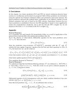
graph of σ. In Figures 2 b-e, we see all the possibilities in the case of n
= L = 6, except for
l
= 1 (self-loop around the kth node).
L = 6
L = 2

L = 3
L = 1 L = 1 L = 1
a
b
c
d
e
f
Fig. 2. Loop number assignment through the choice of different feeback controllers.
We realize that with only one control variable appearing in only one of the components of
the system g, we can set the loop number of the closed-loop system h
f
i
to be equal to any
of the possible values (out of the set D
(L)) by choosing among the feedback controllers f
i
,
i
= 1, , n, defined above. This proves that the type of systems we are considering here are
indeed completely loop number controllable. Moreover, as illustrated in Figure 2 f, if the
control variable u would appear in another component function of g, we may loose the loop
number controllability. Again, due to the structural similarity (see Remark 53), this complete
loop number controllability statement is valid for strongly dependent systems.
In the light of Theorem 47 (see Remark 48), for the stabilization
13
problem we can consider
arbitrary Boolean monomial control systems g : F
n
2

× F
m
2
→ F
n
2
, maybe only requiring the
obvious condition that the mapping σ is not already a fixed point system. Moreover, the
statement of Theorem 47 is telling us that such a system will be stabilizable if and only if the
component functions g
j
depend in such a way on control variables u
i
, that every strongly
connected component of the dependency graph of σ can be forced into loop number one by
incorporating suitable additional edges. This corresponds to the choice of a suitable feedback
controller. The details and proof of this stabilizability statement as well as a brief description
of a stabilization procedure can be found in Delgado-Eckert (2009b).
13
Note that in contrast to the definition of stability introduced in Subsection 1.2.1, in this context we refer
to stabilizability as the property of a control system to become a fixed point system through the choice
of a suitable feedback controller.
474
Discrete Time Systems
4. Conclusions
In this chapter we considered discrete event systems within the paradigm of algebraic state
space models. As we pointed out, traditional approaches to system analysis and controller
synthesis that were developed for continuous and discrete time dynamical systems may not
be suitable for the same or similar tasks in the case of discrete event systems. Thus, one of
the main challenges in the field of discrete event systems is the development of appropriate

mathematical techniques. Finding new mathematical indicators that characterize the dynamic
properties of a discrete event system represents a promising approach to the development of
new analysis and controller synthesis methods.
We have demonstrated how mathematical objects or magnitudes such as invariant
polynomials, elementary divisor polynomials, and the loop number can play the role of the
aforementioned indicators, characterizing the dynamic properties of certain classes of discrete
event systems. Moreover, we have shown how these objects or magnitudes can be used to
effectively address controller synthesis problems for linear modular systems over the finite
field F
2
and for Boolean monomial systems.
We anticipate that the future development of the discrete event systems field will not only
comprise the derivation of new mathematical methods, but also will be concerned with the
development of efficient algorithms and their implementation.
5. References
Baccelli, F., Cohen, G., Olsder, G. & Quadrat, J P. (1992). Synchronisation and linearity, Wiley.
Booth, T. L. (1967). Sequential Machines and Automata Theory, Wiley, New York.
Brualdi, R. A. & Ryser, H. J. (1991). Combinatorial matrix theory, Vol. 39 of Encyclopedia of
Mathematics and its Applications, Cambridge University Press, Cambridge.
Caillaud, B., Darondeau, P., Lavagno, L. & Xie, X. (2002). Synthesis and Control of Discrete Event
Systems, Springer.
Cassandras, C. G. & Lafortune, S. (2006). Introduction to Discrete Event Systems, Springer-Verlag
New York, Inc., Secaucus, NJ, USA.
Colón-Reyes, O., Jarrah, A. S., Laubenbacher, R. & Sturmfels, B. (2006). Monomial dynamical
systems over finite fields, Complex Systems 16(4): 333–342.
Colón-Reyes, O., Laubenbacher, R. & Pareigis, B. (2004). Boolean monomial dynamical
systems, Ann. Comb. 8(4): 425–439.
Delgado-Eckert, E. (2008). Monomial Dynamical and Control Systems over a Finite
Field and Applications to Agent-based Models in Immunology, PhD thesis,
Technische Universität München, Munich, Germany. Available online at

/>Delgado-Eckert, E. (2009a). An algebraic and graph theoretic framework to study monomial
dynamical systems over a finite field, Complex Systems 18(3): 307–328.
Delgado-Eckert, E. (2009b). Boolean monomial control systems, Mathematical and Computer
Modelling of Dynamical Systems 15(2): 107 – 137.
URL: />Delgado-Eckert, E. (2009c). Reverse engineering time discrete finite dynamical systems: A
feasible undertaking?, PLoS ONE 4(3): e4939.
Denardo, E. V. (1977). Periods of Connected Networks and Powers of Nonnegative Matrices,
Mathematics of Operations Research 2(1): 20–24.
Dicesare, F. & Zhou, M. (1993). Petri Net Synthesis for Discrete Event Control of Manufacturing
Systems, Kluwer.
Germundsson, R. (1995). Symbolic Systems — Theory, Computation and Applications, PhD thesis,
Linköping.
475
Discrete Time Systems with Event-Based Dynamics:
Recent Developments in Analysis and Synthesis Methods
Gill, A. (1966). Linear Sequential Circuits: Analysis, Synthesis, and Applications, McGraw-Hill,
New York.
Gill, A. (1969). Linear modular systems, in L. A. Zadeh & E. Polak (eds), System Theory,
McGraw-Hill, New York.
Hopcroft, J. & Ullman, J. (1979). Introduction to automata theory, languages and computation,
Addison-Wesley, Reading .
Iordache, M. V. & Antsaklis, P. J. (2006). Supervisory Control of Concurrent Systems: A Petri Net
Structural Approach, Birkhauser, Boston.
Kailath, T. (1980). Linear Systems, Prentice Hall, Englewood Cliffs.
Kumar, P. R. & Varaiya, P. P. (1995). Discrete Event Systems, Manufacturing Systems, and
Communication Networks, Springer Verlag, NY.
Lancaster, P. & Tismenetsky, M. (1985). The theory of matrices, Computer Science and Applied
Mathematics, second edn, Academic Press Inc., Orlando, FL.
Le Borgne, M., Benveniste, A. & Le Guernic, P. (1991). Polynomial dynamical systems over
finite fields, in G. Jacob & F. Lamnabhi-Lagarrigue (eds), Lecture Notes in Computer

Science, Vol. 165, Springer, Berlin, pp. 212–222.
Lidl, R. & Niederreiter, H. (1997). Finite fields, Vol. 20 of Encyclopedia of Mathematics and its
Applications, second edn, Cambridge University Press, Cambridge. With a foreword
by P. M. Cohn.
Murata, T. (1989). Petri nets: Properties, analysis and applications, Proceedings of the IEEE
77(4): 541 –580.
Plantin, J., Gunnarsson, J. & Germundsson, R. (1995). Symbolic algebraic discrete systems
theory-applied to a fighter aircraft, Decision and Control, IEEE Conference on, Vol. 2,
pp. 1863 –1864 vol.2.
Pták, V. & Sedlaˇcek, I. (1958). On the index of imprimitivity of nonnegative matrices,
Czechoslovak Math. J 8(83): 496–501.
Ramadge, P. & Wonham, W. (1989). The control of discrete event systems, Proceedings of the
IEEE 77(1): 81 –98.
Reger, J. (2004). Linear Systems over Finite Fields – Modeling, Analysis, and Synthesis,
PhD thesis, Lehrstuhl für Regelungstechnik, Friedrich-Alexander-Universität
Erlangen-Nürnberg.
Reger, J. & Schmidt, K. (2004). A finite field framework for modelling, analysis and control
of finite state automata, Mathematical and Computer Modelling of Dynamical Systems
10(3–4): 253–285.
Smale, S. (1998). Mathematical problems of the next century, The Mathematical Intelligencer
20(2): 7–15.
Sontag, E. D. (1998). Mathematical control theory,Vol.6ofTexts in Applied Mathematics, second
edn, Springer-Verlag, New York. Deterministic finite-dimensional systems.
Wolovich, W. A. (1974). Linear Multivariable Systems, Springer, New York.
Young, S. & Garg, V. (1993). On self-stabilizing systems: an approach to the specification and
design of fault tolerant systems, Decision and Control, IEEE Conference on, pp. 1200
–1205 vol.2.
476
Discrete Time Systems
Mihaela Neam¸tu and Dumitru Opri¸s

W est University of Timi¸soara
Romania
1. Introduction
The dynamical systems with discrete time and delay are obtained by the discretization of the
systems of differential equations with delay, or by modeling some processes in which the time
variable is n
∈ IN and the state variables at the moment n −m,wherem ∈ IN , m ≥ 1, are taken
into consideration.
The processes from this chapter have as mathematical model a system of equations given by:
x
n+1
= f (x
n
, x
n−m
, α),(1)
where x
n
= x(n) ∈ IR
p
, x
n−m
= x(n − m) ∈ IR
p
, α ∈ IR and f : IR
p
× IR
p
× IR → IR
p

is a
seamless function, n, m
∈ IN with m ≥ 1. The properties of function f ensure that there is
solution for system (1). The system of equations (1) is called system with discrete-time and delay.
The analysis of the processes described by system (1) follows these steps.
Step 1. Modeling the process.
Step 2. Determining the fixed points for
(1).
Step 3. Analyzing a fixed point of
(1) by studying the sign of the characteristic equation of the
linearized equation in the neighborhood of the fixed point.
Step 4. Determining the value α
= α
0
for which the characteristic equation has the roots
μ
1
(α
0
)=μ(α
0
), μ
2
(α
0
)=
μ(α
0
) with their absolute value equal to 1, and the other roots with
their absolute value less than 1 and the following formulas:

d
|μ(α)|
dα



α=α
0
= 0, μ(α
0
)
k
= 1, k = 1, 2, 3, 4
hold.
Step 5. Determining the local center manifold W
c
loc
(0):
y
= zq + z q +
1
2
w
20
z
2
+ w
11
zz +
1

2
w
02
z
2
+
where z
= x
1
+ ix
2
,with(x
1
, x
2
) ∈ V
1
⊂ IR
2
,0∈ V
1
, q an eigenvector corresponding to
the eigenvalue μ
(0) and w
20
, w
11
, w
02
are vectors that can be determined by the invariance

Discrete Deterministic and Stochastic
Dynamical Systems with Delay - Applications
26
condition of the manifold W
c
loc
(0) with respect to the transformation x
n−m
= x
1
, , x
n
= x
m
,
x
n+1
= x
m+1
. The restriction of system (1) to the manifold W
c
loc
(0) is:
z
n+1
= μ(α
0
)z
n

+
1
2
g
20
z
2
n
+ g
11
z
n
z
n
+
1
2
g
02
z
2
n
+ g
21
z
2
n
z
n
/2, (2)

where g
20
, g
11
, g
02
, g
21
are the coefficients obtained using the expansion in Taylor series
including third-order terms of function f .
System (2) is topologically equivalent with the prototype of the 2-dimensional discrete
dynamic system that characterizes the systems with a Neimark–Sacker bifurcation.
Step 6. Representing the orbits for system (1). The orbits of system (1) in the neighborhood of
the fixed point x
∗
are given by:
x
n
= x
∗
+ z
n
q +
¯
z
n
¯
q
+
1

2
r
20
z
2
n
+ r
11
z
n
¯
z
n
+
1
2
r
02
¯
z
2
n
(3)
where z
n
is a solution of (2) and r
20
, r
11
, r

02
are determined with the help of w
20
, w
11
, w
02
.
The properties of orbit (3) are established using the Lyapunov coefficient l
1
(0).Ifl
1
(0) < 0
then orbit (3) is a stable invariant closed curve (supercritical) and if l
1
(0) > 0thenorbit(3)is
an unstable invariant closed curve (subcritical).
The perturbed stochastic system corresponding to (1) is given by:
x
n+1
= f (x
n
, x
n−m
, α)+g(x
n
, x
n−m
)ξ
n

,(4)
where x
n
= x
0
n
, n ∈ I = {−m, −m + 1, , −1, 0} is the initial segment to be F
0
-measurable,
and ξ
n
is a random variable with E(ξ
n
)=0, E(ξ
2
n
)=σ > 0andα is a real parameter.
System (4) is called discrete-time stochastic system with delay.
For the stochastic discrete-time system with delay, the stability in mean and the stability in
square mean for the stationary state are done.
This chapter is organized as follows. In Section 2 the discrete-time deterministic and
stochastic dynamical systems are defined. In Section 3 the Neimark-Sacker bifurcation for
the deterministic and stochastic Internet control congestion with discrete-time and delay
is studied. Section 4 presents the deterministic and stochastic economic games with
discrete-time and delay. In Section 5, the deterministic and stochastic Kaldor model with
discrete-time is analyzed. Finally some conclusions and future prospects are provided.
For the models from the above sections we establish the existence of the Neimark-Sacker
bifurcation and the normal form. Then, the invariant curve is studied. We also associate
the perturbed stochastic system and we analyze the stability in square mean of the solutions
of the linearized system in the fixed point of the analyzed system.

2. Discrete-time dynamical systems
2.1 The definition of the discrete-time, deterministic and stochastic systems
We intuitively describe the dynamical system concept. We suppose that a physical or biologic
or economic system etc., can have different states represented by the elements of a set S. These
states depend on the parameter t called time. If the system is in the state s
1
∈ S, at the moment
t
1
and passes to the moment t
2
in the state s
2
∈ S, then we denote this transformation by:
Φ
t
1
,t
2
(s
1
)=s
2
478
Discrete Time Systems
and Φ
t
1
,t
2

: S → S is called evolution operator. In the deterministic evolutive processes the
evolution operator Φ
t
1
,t
2
, satisfies the Chapman-Kolmogorov law:
Φ
t
3
,t
2
◦Φ
t
2
,t
1
= Φ
t
3
,t
1
, Φ
t,t
= id
S
.
For a fixed state s
0
∈ S, application Φ : IR → S,definedbyt → s

t
= Φ
t
(s
0
), determines a
curve in set S that represents the evolution of state s
0
when time varies from −∞ to ∞.
An evolutive system in the general form is given by a subset of S
×S that is the graphic of the
system:
F
i
(t
1
, t
2
, s
1
, s
2
)=0, i = 1 n
where F
i
: IR
2
×S → IR.
In what follows, the arithmetic space IR
m

is considered to be the states’space of a system, and
the function Φ is a C
r
-class differentiable application.
An explicit differential dynamical system of C
r
class, is the homomorphism of groups Φ :
(IR, +) → (Di f f
r
(IR
m
), ◦) so that the application IR × IR
m
→ IR
m
defined by (t, x) → Φ( t)(x)
is a differentiable of C
r
-class and for all x ∈ IR
m
fixed, the corresponding application
Φ
(x) : IR → IR
m
is C
r+1
-class.
A differentiable dynamical system on R
m
describes the evolution in continuous time of a

process. Due to the fact that it is difficult to analyze the continuous evolution of the state
x
0
, the analysis is done at the regular periods of time, for example at t = −n, , −1,0, 1, ,n.
If we denote by Φ
1
= f ,wehave:
Φ
1
(x
0
)=f (x
0
), Φ
2
(x
0
)=f
(2)
(x
0
), ,Φ
n
(x
0
)=f
(n)
(x
0
),

Φ
−1
(x
0
)=f
(−1)
(x
0
), ,Φ
−n
(x
0
)=f
(−n)
(x
0
),
where f
(2)
= f ◦ f , ,f
(n)
= f ◦ ◦ f , f
−(n)
= f
(−1)
◦ ◦ f
(−1)
.
Thus, Φ is determined by the diffeomorphism f
= Φ

1
.
A C
r
-class differential dynamical system with discrete time on IR
m
, is the homomorphism of
groups Φ :
(Z, +) → (Di f f
r
(IR
m
), ◦).
The orbit through x
0
∈ IR
m
of a dynamical system with discrete-time is:
O
f
(x
0
)={ , f
−(n)
(x
0
), , f
(−1)
(x
0

), x
0
, f (x
0
), , f
(n)
(x
0
), } = {f
(n)
(x
0
)}
n∈Z
.
Thus O
f
(x
0
) represents a sequences of images of the studied process at regular periods of
time.
For the study of a dynamical system with discrete time, the structure of the orbits’set is
analyzed. For a dynamical system with discrete time with the initial condition x
0
∈ IR
m
(m =
1, 2, 3) we can represent graphically the points of the form x
n
= f

n
(x
0
) for n iterations of the
thousandth or millionth order. Thus, a visual geometrical image of the orbits’set structure
is created, which suggests some properties regarding the particularities of the system. Then,
these properties have to be approved or disproved by theoretical or practical arguments.
An explicit dynamical system with discrete time has the form:
x
n+1
= f (x
n−p
, x
n
), n ∈ IN ,(5)
where f : IR
m
× IR
m
→ IR
m
, x
n
∈ IR
m
, p ∈ IN is fixed, and the initial conditions are x
−p
, x
1−p
,

, x
0
∈ IR
m
.
479
Discrete Deterministic and Stochastic Dynamical Systems with Delay - Applications
For system (5), we use the change of variables x
1
= x
n−p
, x
2
= x
n−(p−1)
, , x
p
= x
n−1
,
x
p+1
= x
n
, and we associate the application
F :
(x
1
, , x
p+1

) ∈ IR
m
× × IR
m
→ IR
m
× × IR
m
given by:
F :
⎛
⎜
⎜
⎜
⎜
⎝
x
1
·
·
x
p
x
p+1
⎞
⎟
⎟
⎟
⎟
⎠

→
⎛
⎜
⎜
⎜
⎜
⎝
x
2
·
·
x
p+1
f (x
1
, x
p+1
)
⎞
⎟
⎟
⎟
⎟
⎠
.
Let
(Ω, F) be a measurable space, where Ω is a set whose elements will be noted by ω and
F is a σ−algebra of subsets of Ω.WedenotebyB(IR) σ−algebra of Borelian subsets of IR. A
random variable is a measurable function X : Ω
→ IR with respect to the measurable spaces

(Ω, F) and (IR, B(IR)) (Kloeden et al., 1995).
A probability measure P on the measurable space
(Ω, F) is a σ−additive function defined on
F with values in [0, 1] so that P(Ω)=1. The triplet (Ω, F, P) is called a probability space.
An arbitrary family ξ
(n, ω)=ξ(n)(ω) of random variables, defined on Ω with values in IR,
is called stochastic process.Wedenoteξ
(n, ω)=ξ(n) for any n ∈ IN and ω ∈ Ω. The functions
X
(·, ω) are called the trajectories of X(n).WeuseE(ξ(n)) for the mean value and E(ξ(n)
2
)
the square mean value of ξ(n) denoted by ξ
n
.
The perturbed stochastic of system (5) is:
x
n+1
= f (x
n−p
, x
n
)+g(x
n
)ξ
n
, n ∈ IN
where g : IR
n
→ IR

n
and ξ
n
is a random variable which satisfies the conditions E(ξ
n
)=0and
E
(ξ
2
n
)=σ > 0.
2.2 Elements used for the study of the discrete-time dynamical systems
Consider the following discrete-time dynamical system defined on IR
m
:
x
n+1
= f (x
n
), n ∈ IN (6)
where f : IR
m
→ IR
m
is a C
r
class function, called vector field.
Some information, regarding the behavior of (6) in the neighborhood of the fixed point, is
obtained studying the associated linear discrete-time dynamical system.
Let x

0
∈ IR
m
be a fixed point of (6). The system
u
n+1
= Df(x
0
)u
n
, n ∈ IN
where
Df
(x
0
)=

∂ f
i
∂x
j

(x
0
), i, j = 1 m
is called the linear discrete-time dynamical system associated to (6) and the fixed point x
0
= f (x
0
).

If the characteristic polynomial of Df
(x
0
) does not have roots with their absolute values equal
to 1, then x
0
is called a hyperbolic fixed point.
We have the following classification of the hyperbolic fixed points:
480
Discrete Time Systems
1. x
0
is a stable point if all characteristic exponents of Df(x
0
) have their absolute values less
than 1.
2. x
0
is an unstable point if all characteristic exponents of Df(x
0
) have their absolute values
greater than 1.
3. x
0
is a saddle point if a part of the characteristic exponents of Df(x
0
) have their absolute
values less than 1 and the others have their absolute values greater than 1.
The orbit through x
0

∈ IR
m
of a discrete-time dynamical system generated by f : IR
m
→ IR
m
is
stable if for any ε
> 0thereexistsδ(ε) so that for all x ∈ B(x
0
, δ(ε)), d( f
n
(x), f
n
(x
0
)) < ε,for
all n
∈ IN .
The orbit through x
0
∈ IR
m
is asymptotically stable if there exists δ > 0sothatforallx ∈
B(x
0
, δ), lim
n→∞
d( f
n

(x), f
n
(x
0
)) = 0.
If x
0
is a fixed point of f, the orbit is formed by x
0
.InthiscaseO(x
0
) is stable (asymptotically
stable) if d
( f
n
(x), x
0
) < ε,foralln ∈ IN and lim
n→∞
f
n
(x)=x
0
.
Let
(Ω, F, P) be a probability space. The perturbed stochastic system of (6) is the following
system:
x
n+1
= f (x

n
)+g(x
n
)ξ
n
where ξ
n
is a random variable that satisfies E(ξ
n
)=0, E(ξ
2
n
)=σ and g(x
0
)=0withx
0
the
fixed point of the system (6).
The linearized of the discrete stochastic dynamical system associated to (6) and the fixed point
x
0
is:
u
n+1
= Au
n
+ ξ
n
Bu
n

, n ∈ IN (7)
where
A
=

∂ f
i
∂x
j

(x
0
), B =

∂g
i
∂x
j

(x
0
), i, j = 1 m.
We use E
(u
n
)=E
n
, E(u
n
u

T
n
)=V
n
, u
n
=(u
1
n
, u
2
n
, ,u
m
n
)
T
.
Proposition 2.1.(i)ThemeanvaluesE
n
satisfy the following system of equations:
E
n+1
= AE
n
, n ∈ IN (8)
(ii) The square mean values satisfy:
V
n+1
= AV

n
A
T
+ σBV
n
B
T
, n ∈ IN (9)
Proof. (i) From (7) and E
(ξ
n
)=0 we obtain (8).
(ii) Using (7) we have:
u
n+1
u
T
n
+1
= Au
n
u
T
n
A
T
+ ξ
n
(Au
n

u
T
n
B
T
+ Bu
n
u
T
n
A
T
)+ξ
2
n
Bu
n
u
T
n
B
T
. (10)
By (10) and E
(ξ
n
)=0, E(ξ
2
n
)=σ we get (9).

Let
¯
A be the matrix of system (8), respectively (9). The characteristic polynomial is given by:
P
2
(λ)=det(λI −
¯
A
).
For system (8), respectively (9), the analysis of the solutions can be done by studying the roots
of the equation P
2
(λ)=0.
481
Discrete Deterministic and Stochastic Dynamical Systems with Delay - Applications
2.3 Discrete-time dynamical systems with one parameter
Consider a discrete-time dynamical system depending on a real parameter α, defined by the
application:
x
→ f (x, α), x ∈ IR
m
, α ∈ IR (11)
where f : IR
m
× IR → IR
m
is a seamless function with respect to x and α.Letx
0
∈ IR
m

be a
fixed point of (11), for all α
∈ IR. The characteristic equation associated to the Jacobian matrix
of the application (11), evaluated in x
0
is P(λ, α)=0, where:
P
(λ, α)=λ
m
+ c
1
(α)λ
m−1
+ ···+ c
m−1
(α)λ + c
m
(α).
The roots of the characteristic equation depend on the parameter α.
The fixed point x
0
is called stable for (11), if there exists α = α
0
so that equation P (λ, α
0
)=0
has all roots with their absolute values less than 1. The existence conditions of the value α
0
,
are obtained using Schur Theorem (Lorenz, 1993).

If m
= 2, the necessary and sufficient conditions that all roots of the characteristic equation
λ
2
+ c
1
(α)λ + c
2
(α)=0 have their absolute values less than 1 are:
|c
2
(α)| < 1, |c
1
(α)| < |c
2
(α)+1|.
If m
= 3, the necessary and sufficient conditions that all roots of the characteristic equation
λ
3
+ c
1
(α)λ
2
+ c
2
(α)λ + c
3
(α)=0
have their absolute values less than 1 are:

1
+ c
1
(α)+c
2
(α)+c
3
(α) > 0, 1 −c
1
(α)+c
2
(α) − c
3
(α) > 0
1
+c
2
(α)−c
3
(α)(c
1
(α)+c
3
(α))> 0, 1−c
2
(α)+c
3
(α)(c
1
(α)−c

3
(α))> 0, |c
3
(α)|< 1.
The Neimark–Sacker (or Hopf) bifurcation is the value α
= α
0
for which the characteristic
equation P
(λ, α
0
)=0 has the roots μ
1
(α
0
)=μ(α
0
), μ
2
(α
0
)=μ(α
0
) in their absolute values
equal to 1, and the other roots have their absolute values less than 1 and:
a)
d|μ(α)|
dα




α=α
0
= 0. b) μ
k
(α
0
) = 1, k = 1, 2, 3, 4
hold.
For the discrete-time dynamical system
x
(n + 1)=f (x(n), α)
with f : IR
m
→ IR
m
, the following statement is true:
Proposition 2.2. ((Kuznetsov, 1995), (Mircea et al., 2004)) Let α
0
be a Neimark-Sacker bifurcation.
The restriction of (11) to two dimensional center manifold in the point
(x
0
, α
0
) has the normal form:
η
→ ηe
iθ
0

(1 +
1
2
d
|η|
2
)+O(≡

)
where η ∈ C,d∈ C.Ifc=Re d = 0 there is a unique limit cycle in the neighborhood of x
0
.The
expression of d is:
d
=
1
2
e
−iθ
0
< v
∗
, C(v, v,
¯
v)+2B(v, (I
m
− A)
−1
B(v,
¯

v)) + B(v, (e
2iθ
0
I
m
− A)
(−1)
B(v, v)) > 0
482
Discrete Time Systems
where Av = e
iθ
0
v, A
T
v
∗
= e
−iθ
0
v
∗
and < v
∗
, v >= 1;A=

∂ f
∂x

(x

0
,α
0
)
,B=

∂
2
f
∂x
2

(x
0
,α
0
)
and
C
=

∂
3
f
∂x
3

(x
0
,α

0
)
.
The center manifold in x
0
is a two dimensional submanifold in IR
m
,tangentinx
0
to the vectorial space
of the eigenvectors v and v
∗
.
The following statements are true:
Proposition 2.3. (i) If m
= 2, the necessary and sufficient conditions that a Neimark–Sacker
bifurcation exists in α
= α
0
are:
|c
2
(α
0
)| = 1, |c
1
(α
0
)| < 2, c
1

(α
0
) = 0, c
1
(α
0
) = 1,
dc
2
(α)
dα



α=α
0
> 0.
(ii) If m
= 3, the necessary and sufficient conditions that a Neimark–Sacker bifurcation exists in
α
= α
0
,are:
|c
3
(α
0
) < 1, c
2
(α

0
)=1 + c
1
(α
0
)c
3
(α
0
) − c
3
(α
0
)
2
,
c
3
(α
0
)(c
1
(α
0
)c

3
(α
0
)+c


1
(α
0
)c
3
(α
0
) − c

2
(α
0
) − 2c
3
(α
0
)c

3
(α
0
))
1 + 2c
2
3
(α
0
) − c
1

(α
0
)c
3
(α
0
)
>
0,
|c
1
(α
0
) − c
3
(α
0
)| = 0, |c
1
(α
0
) − c
3
(α
0
)| = 1.
In what follows, we highlight the normal form for the Neimark–Sacker bifurcation.
Theorem 2.1. (The Neimark–Sacker bifurcation). Consider the two dimensional discrete-time
dynamical system given by:
x

→ f (x, α), x ∈ IR
2
, α ∈ IR (12)
with x
= 0, fixed point for all |α| small enough and
μ
12
(α)=r(α)e
±iϕ(θ)
where r(0)=1, ϕ(0)=θ
0
. If the following conditions hold:
c
1
: r

(0) = 0, c
2
: e
ikθ
0
= 1, k = 1, 2, 3, 4
then there is a coordinates’transformation and a parameter change so that the application (12) is
topologically equivalent in the neighborhood of th e origin with the system:

y
1
y
2


→

cos θ
(β) −sin θ(β)
sin θ(β) cos θ(β)


(1 + β)

y
1
y
2

+
+(
y
2
1
+ y
2
2
)

a
(β) −b(β)
b(β) a(β)

y
1

y
2

+ O(†

),
where θ
(0)=θ
0
,a(0)=Re(e
−iθ
0
C
1
(0)),and
C
1
(0)=
g
20
(0)g
11
(0)(1 −2μ
0
)
2(μ
2
0
−μ
0

)
+
|
g
11
(0)|
2
1 − μ
0
+
|
g
02
(0)|
2
2(μ
2
0
−μ
0
)
+
g
21
(0)
2
μ
0
= e
iθ

0
,g
20
, g
11
, g
02
, g
21
are the coefficients obtained using the expansion in Taylor series including
third-order terms of function f .
483
Discrete Deterministic and Stochastic Dynamical Systems with Delay - Applications
2.4 The Neimark-Sacker bifurcation for a class of discrete-time dynamical systems with
delay
A two dimensional discrete-time dynamical system with delay is defined by the equations
x
n+1
= x
n
+ f
1
(x
n
, y
n
, α)
y
n+1
= y

n
+ f
2
(x
n−m
, y
n
, α)
(13)
where α
∈ IR, f
1
, f
2
: IR
3
→ IR are seamless functions, so that for any |α| small enough, the
system f
1
(x, y, α)=0, f
2
(x, y, α)=0, admits a solution (x, y)
T
∈ IR
2
.
Using the translation x
n
→ x
n

+ x, y
n
→ y
n
+ y, and denoting the new variables with the
same notations x
n
, y
n
, system (13) becomes:
x
n+1
= x
n
+ f (x
n
, y
n
, α)
y
n+1
= y
n
+ g(x
n−m
, y
n
, α)
(14)
where:

f
(x
n
, y
n
, α)=f
1
(x
n
+ x, y
n
+ y, α); g (x
n−m
, y
n
, α)=f
2
(x
n−m
+ x, y
n
+ y, α).
With the change of variables x
1
= x
n−m
, x
2
= x
n−(m−1)

, ,x
m
= x
n−1
, x
m+1
= x
n
, x
m+2
=
y
n
, application (14) associated to the system is:
⎛
⎜
⎜
⎜
⎜
⎜
⎝
x
1
x
2
.
.
.
x
m+1

x
m+2
⎞
⎟
⎟
⎟
⎟
⎟
⎠
→
⎛
⎜
⎜
⎜
⎝
x
2
.
.
.
x
m+1
+ f (x
m+1
, x
m+2
, α)
x
m+2
+ g(x

1
, x
m+2
, α)
⎞
⎟
⎟
⎟
⎠
. (15)
We use the notations:
a
10
=
∂ f
∂x
m+1
(0, 0, α), a
01
=
∂ f
∂x
m+2
(0, 0, α),
b
10
=
∂g
∂x
1

(0, 0, α), b
01
=
∂g
∂x
m+2
(0, 0, α)
a
20
=
∂
2
f
∂x
m+1
∂x
m+1
(0, 0, α), a
11
=
∂
2
f
∂x
m+1
∂x
m+2
(0, 0, α),
a
02

=
∂
2
f
∂x
m+2
∂x
m+2
(0, 0, α), a
30
=
∂
3
f
∂x
m+1
∂x
m+1
∂x
m+1
(0, 0, α),
a
21
=
∂
3
f
∂x
m+1
∂x

m+1
∂x
m+2
(0, 0, α), a
12
=
∂
3
f
∂x
m+1
∂x
m+2
∂x
m+2
(0, 0, α),
a
03
=
∂
3
f
∂x
m+2
∂x
m+2
∂x
m+2
(0, 0, α)
(16)

484
Discrete Time Systems
b
20
=
∂
2
g
∂x
1
∂x
1
(0, 0, α), b
11
=
∂
2
g
∂x
1
∂x
m+2
(0, 0, α),
b
02
=
∂
2
g
∂x

m+2
∂x
m+2
(0, 0, α), b
30
=
∂
3
g
∂x
1
∂x
1
∂x
1
(0, 0, α),
b
21
=
∂
3
g
∂x
1
∂x
1
∂x
m+2
(0, 0, α), b
12

=
∂
3
g
∂x
1
∂x
m+2
∂x
m+2
(0, 0, α),
b
03
=
∂
3
g
∂x
m+2
∂x
m+2
∂x
m+2
(0, 0, α).
(17)
With (16) and (17) from (15) we have:
Proposition 2.4. ((Mircea et al., 2004)) (i) The Jacobian matrix associated to (15) in (0, 0)
T
is:
A

=
⎛
⎜
⎜
⎜
⎜
⎜
⎝
0 1 0 0
0 0 0 0
.
.
.
.
.
.
.
.
.
.
.
.
0 0 1
+ a
10
a
01
b
10
0 0 1+ b

01
⎞
⎟
⎟
⎟
⎟
⎟
⎠
. (18)
(ii) The characteristic equation of A is:
λ
m+2
−(2 + a
10
+ b
01
)λ
m+1
+(1 + a
10
)(1 + b
01
)λ −a
01
b
10
= 0. (19)
(iii) If μ
= μ(α) is an eigenvalue of (19), then the eigenvector q ∈ C
m+2

, solution of the system
Aq
= μq, has the components:
q
1
= 1, q
i
= μ
i−1
, i = 2, ,m + 1, q
m+2
=
b
10
μ −1 −b
01
. (20)
The eigenvector p
∈ C
m+2
defined by A
T
p = μp has the components
p
1
=
(
μ −1 − a
10
)(μ −1 −b

01
)
m(μ −1 −a
10
)(μ −1 −b
01
)+μ(2μ −2 − a
10
−b
01
)
, p
i
=
1
μ
i−1
p
1
, i = 2, ,m,
p
m+1
=
1
μ
m−1
(μ −1 − a
10
)
p

1
, p
m+2
=
μ
b
10
p
1
.
(21)
The vectors q, p satisfy the condition:
< q, p >=
m+2
∑
i=1
q
i
p
i
= 1.
The proof is obtained by straight calculation from (15) and (18).
The following hypotheses are taken into account:
H
1
. The characteristic equation (19) has one pair of conjugate eigenvalues μ(α), μ(α) with
their absolute values equal to one, and the other eigenvalues have their absolute values less
than one.
485
Discrete Deterministic and Stochastic Dynamical Systems with Delay - Applications

H
2
. The eigenvalues μ(α), μ(α) intersect the unit circle for α = 0, and satisfy the transversality
condition
d
dα
|μ(α)|
α=0
= 0.
H
3
.Ifarg(μ(α)) = θ(α),andθ
0
= θ(0),thene
iθ
0
k
= 1, k = 1, 2, 3, 4.
From H
2
we notice that for all |α| small enough, μ(α) is given by:
μ
(α)=r(α)e
iθ(α)
with r(0)=1, θ(0)=θ
0
, r

(0) = 0. Thus r(α)=1 + β(α) where β(0)=0andβ


(0) = 0.
Taking β as a new parameter, we have:
μ
(β)=(1 + β)e
iθ(β)
(22)
with θ
(0)=θ
0
. From (22) for β < 0 small enough, the eigenvalues of the characteristic
equation (19) have their absolute values less than one, and for β
> 0smallenough,the
characteristic equation has an eigenvalue with its absolute value greater than one. Using
the center manifold Theorem (Kuznetsov, 1995), application (15) has a family of invariant
manifolds of two dimension depending on the parameter β. The restriction of application (15)
to this manifold contains the essential properties of the dynamics for (13). The restriction of
application (15) is obtained using the expansion in Taylor series until the third order of the
right side of application (15).
2.5 The center manifold, the normal f orm
Consider the matrices:
A
1
=

a
20
a
11
a
11

a
02

, C
1
=

a
30
a
21
a
21
a
12

, D
1
=

a
21
a
12
a
12
a
03

A

2
=

b
20
b
11
b
11
b
02

, C
2
=

b
30
b
21
b
21
b
12

, D
2
=

b

21
b
12
b
12
b
03

with the coefficients given by (16) and (17).
Denoting by x
=(x
1
, ,x
m+2
) ∈ IR
m+2
, application (15), is written as x → F(x),where
F
(x)=(x
2
, ,x
m
, x
m+1
+ f (x
m+1
, x
m+2
, α), x
m+2

+ g(x
1
, x
m+2
, α)).
The following statements hold:
Proposition 2.5. (i) The expansion in Taylor series until the third order of function F
(x) is:
F
(x)=Ax +
1
2
B
(x, x)+
1
6
C
(x, x, x)+O(|§|

), (23)
where A is the matrix (18), and
B
(x, x)=(0, ,0,B
1
(x, x), B
2
(x, x))
T
,
C

(x, x, x)=(0, ,0,C
1
(x, x, x), C
2
(x, x, x))
T
,
486
Discrete Time Systems
where:
B
1
(x, x)=(x
m+1
, x
m+2
)A
1

x
m+1
x
m+2

, B
2
(x, x)=(x
1
, x
m+2

)A
2

x
1
x
m+2

,
C
1
(x, x, x)=(x
m+1
, x
m+2
)(x
m+1
C
1
+ x
m+2
D
1
)

x
m+1
x
m+2


,
C
2
(x, x, x)=(x
1
, x
m+2
)(x
1
C
2
+ x
m+2
D
2
)

x
1
x
m+2

.
(24)
(ii) Any vector x
∈ IR
m+2
admits the decomposition:
x
= zq + z q + y, z ∈ C (25)

where zq
+ z q ∈ T
center
,y∈ T
stable
;T
center
is the vectorial space generated by the eigenvectors
corresponding to the eigenvalues of the characteristic equation (19) with their absolute values equal to
one and T
stable
is the vectorial subspace generated by the eigenvectors corresponding to the eigenvalues
of the characteristic equation (19) with their absolute values less than 1. Moreover:
z
=< p, x >, y = x− < p, x > q− < p, x > q. (26)
(iii) F
(x) given by (23) has the decomposition:
F
(x)=F
1
(z, z)+F
2
(y)
where
F
1
(z, z)=G
1
(z)q + G
1

(z
1
)q+ < p, N(zq + z q + y) > q+ < p, N(zq + z q + y) > q
G
1
(z)=μz+ < p, N(zq + z q + y) >
F
2
(y)=Ay + N(zq + z q + y)− < p, N(zq + z q + y) > q− < p, N(zq + z q + y) > q
(27)
and
N
(zq + z q + y)=
1
2
B
(zq + z q + y , zq + z q + y)+
+
1
6
C
(zq + z q + y, zq + z q + y, zq + z q + y)+O(zq + zq + y)
(28)
(iv) The two-dimensional differential submanifold from IR
m+2
,givenbyx= zq + z q + V(z, z),z∈
V
0
⊂ C,whereV(z, z)=V(z, z), < p, V(z, z) >= 0,
∂V

(z, z)
∂z
(0, 0)=0, is tangent to the vectorial
space T
center
in 0 ∈ C.
Proof. (i) Taking into account the expression of F
(x) we obtain the expansion in Taylor series
until the third order (23).
(ii) Because IR
m+2
= T
center
⊕ T
stable
and < p, y >= 0, for any y ∈ T
stable
, we obtain (25) and
(26).
(iii) Because F
(x) ∈ IR
m+2
, with decomposition (25) and < p, q >= 1, < p, q >= 0, we have
(27).
(iv) Using the definition of the submanifold, this submanifold is tangent to T
center
.
487
Discrete Deterministic and Stochastic Dynamical Systems with Delay - Applications
The center manifold in (0, 0)

T
∈ IR
2
is a two dimensional submanifold from IR
m+2
tangent to
T
center
at 0 ∈ C and invariant with respect to the applications G
1
and F
2
, given by (27). If
x
= zq + z q + V(z, z), z ∈V
0
⊂ C is the analytical expression of the tangent submanifold to
T
center
, the invariant condition is written as:
V
(G
1
(z), G
1
(z)) = F
2
(V(z, z)). (29)
From (27), (28) and (29) we find that x
= zq + z q + V(z, z), z ∈V

0
is the center manifold if
and only if the relation:
V
(μz+ < p, N(zq + z q + V(z, z) >, μz+ < p, N(zq + z q + V(z, z)) >)=AV (z, z)+
+
N(zq + z q+V(z, z))−< p, N(zq+z q + V(z, z)) > q−< p, N(zq +z q+V(z, z)) > q
(30)
holds.
In what follows we consider the function V
(z, z) of the form:
V
(z, z)=
1
2
w
20
z
2
+ w
11
zz + w
02
z
2
+ O(|‡|

),‡∈V

∈IC. (31)

Proposition 2.6. (i) If V
(z, z) is given by (31), and N(zq + z q + y),withy= V(z, z) is given by
(28), then:
G
1
(z)=μz +
1
2
g
20
z
2
+ g
11
zz + g
02
z
2
+
1
2
g
21
z
2
z + (32)
where:
g
20
=< p, B(q, q) >, g

11
=< p, B(q, q) >, g
02
=< p, B(q, q) >
g
21
=< p, B(q, w
20
) > +2 < p, B(q, w
11
) > + < p, C(q, q, q) > .
(33)
(ii) If V
(z, z) is given by (31), relation (30) holds, if and only if w
20
, w
11
, w
02
satisfy the relations:
(μ
2
I − A)w
20
= h
20
, (I − A)w
11
= h
11

, (μ
2
I − A)w
02
= h
02
(34)
where:
h
20
= B(q, q)− < p, B(q, q) > q− < p, B(q, q) > q
h
11
= B(q, q)− < p, B(q, q) > q− < p, B(q, q) > q
h
02
= B(q, q)− < p, B(q, q) > q− < p, B(q, q ) > q.
Proof. (i) Because B
(x, x) is a bilinear form, C(x, x, x) is a trilinear form, and y = V(z, z),from
(28) and the expression of G
1
(z) given by (27), we obtain (32) and (33).
(ii) In (30), replacing V
(z, z) with (32) and N(zq + z q + V(z, z)) given by (28), we find that
w
20
, w
11
, w
02

satisfy the relations (31).
Let q
∈ IR
m+2
, p ∈ IR
m+2
be the eigenvectors of the matrices A and A
T
corresponding to the
eigenvalues μ and
μ given by (20) and (21) and:
a
= B
1
(q, q), b = B
2
(q, q), a
1
= B
1
(q, q), b
1
= B
2
(q, q), C
1
= C
1
(q, q, q), C
2

= C
2
(q, q, q),
r
1
20
= B
1
(q, w
20
), r
2
20
= B
2
(q, w
20
), r
1
11
= B
1
(q, w
11
), r
2
11
= B
2
(q, w

11
),
(35)
488
Discrete Time Systems
where B
1
, B
2
, C
1
, C
2
, are applications given by (24).
Proposition 2.7. (i) The coefficients g
20
, g
11
, g
02
given by (33) have the expressions:
g
20
= p
m+1
a + p
m+2
b, g
11
= p

m+1
a
1
+ p
m+2
b
1
, g
02
= p
m+1
a + p
m+2
b. (36)
(ii) The vectors h
20
, h
11
, h
02
given by (34) have the expressions:
h
20
=(0, ,0,a, b)
T
−(p
m+1
a + p
m+2
b)q − (p

m+1
a + p
m+2
b)q
h
11
=(0, ,0,a, b)
T
−(p
m+1
a
1
+ p
m+2
b
1
)q −(p
m+1
a
1
+ p
m+2
b)q
h
02
= h
20
.
(37)
(iii) The systems of linear equations (34) have the solutions:

w
20
=

v
1
20
, μ
2
v
1
20
, ,μ
2m
v
1
20
,
a
+(μ
2
− a
10
)μ
2m
v
1
20
a
01


T
−
p
m+1
a + p
m+2
b
μ
2
−μ
q
−
p
m+1
a + p
m+2
μ
2
−μ
q
w
11
=

v
1
11
, v
1

11
, ,v
1
11
,
a
1
+(1 − a
10
)v
1
11
a
01

T
−
p
m+1
a
1
+ p
m+2
b
1
1 − μ
q
−
p
m+1

a
1
+ p
m+2
b
1
1 − μ
q
w
02
=
w
20
, v
1
20
=
aa
01
−b(μ
2
−b
01
)
(μ
2
− a
10
)(μ
2

−b
01
)μ
2m
−b
10
a
01
, v
1
11
=
b
1
a
01
− a
1
(1 − b
01
)
(1 − a
10
)(1 −b
01
) − b
10
a
01
.

(iv) The coefficient g
21
given by (33) has the expression:
g
21
= p
m+1
r
1
20
+ p
m+2
r
2
20
+ 2(p
m+1
r
1
11
+ p
m+2
r
2
11
)+p
m+1
C
1
+ p

m+2
C
2
. (38)
Proof. (i) The expressions from (36) are obtained from (33) using (35).
(ii) The expressions from (37) are obtained from (34) with the notations from (35).
(iii) Because μ
2
,
μ
2
, 1 are not roots of the characteristic equation (19) then the linear systems
(34) are determined compatible systems. The relations (37) are obtained by simple calculation.
(iv) From (33) with (35) we obtain (38).
Consider the discrete-time dynamical system with delay given by (13), for which the roots of
the characteristic equation satisfy the hypotheses H
1
, H
2
, H
3
. The following statements hold:
Proposition 2.8. (i) The solution of the system (13) in the neighborhood of the fixed point
(x, y) ∈ IR
2
,
is:
x
n
=

x + q
m+1
z
n
+ q
m+1
z
n
+
1
2
w
m+1
20
z
2
n
+ w
m+1
11
z
n
z
n
+
1
2
w
m+1
02

z
2
n
y
n
= y + q
m+2
z
n
+ q
m+2
z
n
+
1
2
w
m+2
20
z
2
n
+ w
m+2
11
z
n
z
n
+

1
2
w
m+2
02
z
2
n
x
n−m
= u
n
= x + q
1
z
n
+ q
1
z
n
+
1
2
w
1
20
z
2
n
+ w

1
11
z
n
z
n
+
1
2
w
1
02
z
2
n
(39)
where z
n
is a solution of the equation:
z
n+1
= μz
n
+
1
2
g
20
z
2

n
+ g
11
z
n
z
n
+
1
2
g
02
z
2
n
+
1
2
g
21
z
2
n
z
n
(40)
489
Discrete Deterministic and Stochastic Dynamical Systems with Delay - Applications
and the coefficients from (40) are given by (36) and (38).
(ii) There is a complex change variable, so that equation (40) becomes:

w
n+1
= μ(β)w
n
+ C
1
(β)w
2
n
w
n
+ O(|
\
|

) (41)
where:
C
1
(β)=
g
20
(β)g
11
(β)(μ(β) −3 −2μ(β))
2(μ(β)
2
−μ(β))(μ(β) −1)
+
|

g
11
(β)|
2
1 − μ(β)
+
|
g
02
(β)|
2
2(μ
2
(β) −μ(β))
+
g
21
(β)
2
.
(iii) Let l
0
= Re(e
−iθ
0
C
1
(0)),whereθ
0
= arg(μ(0)).Ifl

0
< 0, in the neighborhood of the fixed point
(
x, y) there is an invariant stable limit cycle.
Proof. (i) From Proposition 2.6, application (15) associated to (13) has the canonical form (40).
A solution of system (40) leads to (39).
(ii) In equation (40), making the following complex variable change
z
= w +
g
20
2(μ
2
−μ)
w
2
+
g
11
|μ|
2
−μ
w
w +
g
02
2(μ
2
−μ)
w

2
+
+
g
30
6(μ
3
−μ)
w
3
+
g
12
2(μ|μ|
2
−μ)
ww
2
+
g
03
6(μ
3
−μ)
w
3
,
for β small enough, equation (41) is obtained. The coefficients g
20
, g

11
, g
02
are given by (36)
and
g
30
= p
m+1
C
1
(q, q, q)+p
m+2
C
2
(q, q, q),
g
12
= p
m+1
C
1
(q, q, q)+p
m+2
C
2
(q, q, q)
g
03
= p

m+1
C
1
(q, q, q)+p
m+2
C
2
(q, q, q).
(iii) The coefficient C
1
(β) is called resonant cubic coefficient, and the sign of the coefficient l
0
,
establishes the existence of a stable or unstable invariant limit cycle (attractive or repulsive)
(Kuznetsov, 1995).
3. Neimark-Sacker bifurcation in a discrete time dynamic system for Internet
congestion.
The model of an Internet network with one link and single source, which can be formulated
as:
˙
x
(t)=k(w − af(x(t − τ))) (42)
where: k
> 0, x(t) is the sending rate of the source at the time t, τ is the sum of forward
and return delays, w is a target (set-point), and the congestion indication function f : IR
+
→
IR
+
is increasing, nonnegative, which characterizes the congestion. Also, we admit that f is

nonlinear and its third derivative exists and it is continuous.
The model obtained by discretizing system (42) is given by:
x
n+1
= x
n
− akf (x
n−m
)+kw (43)
for n, m
∈ IN , m > 0 and it represents the dynamical system with discrete-time for Internet
congestion with one link and a single source.
490
Discrete Time Systems
Using the change of variables x
1
= x
n−m
, , x
m
= x
n−1
, x
m+1
= x
n
, the application
associated to (43) is:
⎛
⎜

⎜
⎜
⎝
x
1
.
.
.
x
m
x
m+1
⎞
⎟
⎟
⎟
⎠
→
⎛
⎜
⎜
⎜
⎝
x
2
.
.
.
x
m+1

kw − akf (x
1
)+x
m+1
⎞
⎟
⎟
⎟
⎠
. (44)
The fixed point of (44) is
(x
∗
, ,x
∗
)
T
∈ IR
m+1
,wherex
∗
satisfies relation w = af(x
∗
).With
the translation x
→ x + x
∗
, application (44) can be written as:
⎛
⎜

⎜
⎜
⎝
x
1
.
.
.
x
m
x
m+1
⎞
⎟
⎟
⎟
⎠
→
⎛
⎜
⎜
⎜
⎝
x
2
.
.
.
x
m+1

kw −ak g(x
1
)+x
m+1
⎞
⎟
⎟
⎟
⎠
(45)
where g
(x
1
)=f (x
1
+ x
∗
).
The following statements hold:
Proposition 3.1. ((Mircea et al., 2004)) (i) The Jacobian matrix of (45) in 0
∈ IR
m+1
is
A
=
⎛
⎜
⎜
⎜
⎜

⎝
0 1 0 0
0 0 1 0

0 0 0 1
−akρ
1
0 0 1
⎞
⎟
⎟
⎟
⎟
⎠
(46)
where ρ
1
= g

(0).
(ii) The characteristic equation of A is:
λ
m+1
−λ
m
+ akρ
1
= 0. (47)
(iii) If μ
∈ C is a root of (47), the eigenvector q ∈ IR

m+1
that corresponds to the eigenvalue μ,ofthe
matrix A, has the components:
q
i
= μ
i−1
, i = 1, ,m + 1
and the components of the eigenvector p
∈ IR
m+1
corresponding to
μ of the matrix A
T
are:
p
1
= −
akρ
1
μ
m+1
−makρ
1
, p
i
=
1
μ
i−1

p
1
, i = 2, ,m −1, p
m
=
μ
2
−μ
pρ
1
p
1
, p
m+1
= −
μ
akρ
1
p
1
.
The vectors p
∈ IR
m+1
,q∈ IR
m+1
satisfy the relation
m+1
∑
i=1

p
i
q
i
= 1.
The following statements hold:
491
Discrete Deterministic and Stochastic Dynamical Systems with Delay - Applications
Proposition 3.2. (i) If m = 2, equation (47) becomes:
λ
3
−λ
2
+ akρ
1
= 0. (48)
Equation (48) has two complex roots with their absolute values equal to 1 and one r oot with the absolute
value less than 1, if and only if k
=
√
5 −1
2aρ
1
.Fork= k
0
=
√
5 −1
2aρ
1

, equation (48) has the roots:
λ
1,2
= exp(±iθ(k
0
)i),
θ
(a
0
)=arccos
1
+
√
5
4
. (49)
(ii) With respect to the change of parameter
k
= k(β)=k
0
+ g(β)
where:
g
(β)=

1 + 4(1 + β)
6
−(1 + β)
2
−

√
5 + 1
2k
0
ρ
1
equation (49) becomes:
λ
3
−λ
2
+ ak(β)ρ
1
= 0. (50)
The roots of equation (50) are:
μ
1,2
(β)=(1 + β)exp (±iω(β)), λ(β)=−
ak(β)ρ
1
(1 + β)
2
where:
ω
(β)=arccos
(1 + β)
2
+

1 + 4(1 + β)

6
4(1 + β)
2
.
(iii) The eigenvector q
∈ IR
3
, associated to the μ = μ(β), for the matrix A has the components:
q
1
= 1, q
2
= μ, q
3
= μ
2
and the eigenvector p ∈ IR
3
associated to the eigenvalue μ = μ(β) for the matrix A
T
has the
components:
p
1
=
akρ
1
2akρ
1
−μ

3
, p
2
=
μ
2
μ
3
−2akρ
1
, p
3
=
μ
μ
3
−2akρ
1
.
(iv) a
0
is a Neimark-Sacker bifurcation point.
Using Proposition 3.2, we obtain:
Proposition 3.3. The solution of equation (43) in the neighborhood of the fixed point x
∗
∈ IRis:
u
n
= x
∗

+ z
n
+ z
n
+
1
2
w
1
20
z
2
n
+ w
1
11
z
n
z
n
+
1
2
w
1
02
z
2
n
x

n
= x
∗
+ q
3
z
n
+ q
3
z
n
+
1
2
w
3
20
z
2
n
+ w
3
11
z
n
z
n
+
1
2

w
3
02
z
2
n
492
Discrete Time Systems
where:
w
1
20
=
μ
2
(μ
2
−1)h
1
20
−(μ
2
−1)h
2
20
+ h
3
20
μ
6

−μ
4
+ akρ
1
, w
2
20
= μ
2
w
1
20
−h
1
20
, w
3
20
= μ
4
w
1
20
−μ
2
h
1
20
−h
2

20
w
1
11
=
h
3
11
akρ
1
, w
2
11
= w
1
11
−h
1
11
, w
3
11
= w
1
11
−h
1
11
−h
2

11
h
1
20
= 4akρ
2
(p
3
+ p
3
), h
2
20
= akρ
1
(p
3
q
2
+ p
3
q
2
), h
3
20
= 4akρ
2
(1 + p
3

q
3
+ p
3
q
3
)
h
1
11
= h
1
20
, h
2
11
= h
2
20
, h
3
11
= h
3
20
and z
n
∈ C is a solution of equation:
z
n+1

= μz
n
−
1
2
p
3
akρ
2
(z
2
n
+ 2z
n
z
n
+ z
2
n
)+
1
2
p
3
(−kaρ
1
w
1
20
−kaρ

1
w
1
11
+ ρ
3
),
rho
1
= f

(0), ρ
2
= f

(0), ρ
3
= f

(0).
Let
C
1
(β)=−
p
3
a
2
k
2

ρ
2
2
(μ −3 −2μ)
2(μ
2
−μ)(μ −1)
+
a
2
k
2
ρ
2
2
|p
3
|
2
1 −μ
+
ak|ρ
2
p
3
|
2(μ
2
−μ)
+

p
3
(−akρ
1
w
1
20
− akρ
1
w
1
11
+ ρ
3
)
and
l
(0)=Re(exp (−iθ(a
0
))C
1
(0)).
If l
(0) < 0, the Neimark–Sacker bifurcation is supercritical (stable).
The model of an Internet network with r links and a single source, can be analyzed in a similar
way.
The perturbed stochastic equation of (43) is:
x
n+1
= x

n
−αkf(x
n−m
)+kw + ξ
n
b(x
n
− x
∗
) (51)
and x
∗
satisfies the relation w = af(x
∗
),whereE(ξ
n
)=0, E(ξ
2
n
)=σ > 0.
We study the case m
= 2. Using (46) the linearized equation of (51) has the matrices:
A
1
=
⎛
⎝
010
001
−akρ

1
01
⎞
⎠
, B
=
⎛
⎝
000
000
00b
⎞
⎠
Using Proposition 2.1, the characteristic polynomial of the linearized system of (51) is given
by:
P
2
(λ)=(λ
3
−(1 + σb
2
)λ
2
− a
2
k
2
ρ
2
1

)(λ
3
+ akρ
1
λ + a
2
k
2
ρ
2
1
).
If the roots of P
2
(λ) have their absolute values less than 1, then the square mean values of the
solutions for the linearized system of (51) are asymptotically stable. The analysis of the roots
for the equation P
2
(λ)=0 can be done for fixed values of the parameters.
The numerical simulation can be done for: w
= 0.1, a = 8andf (x)=x
2
/(20 −3x).
493
Discrete Deterministic and Stochastic Dynamical Systems with Delay - Applications