Heat Transfer Mathematical Modelling Numerical Methods and Information Technology Part 7 doc

Fast BEM Based Methods for Heat Transfer Simulation 21
A hotstrip in a cavity produces two vortices, one on each side. For Ra ≤ 10
5
the flow field is
symmetric in the case of central placement of the hotstrip. Symmetry is lost when hotstrip is
place off-centre. Most of the heat is transferred from the sides of the hotstrip and only a small
part from the top wall.
Introduction of nanofluids leads to enhanced heat transfer in all cases. The enhancement
is largest when conduction is the dominant heat transfer mechanism, since in this case the
increased heat conductivity of the nanofluid is important. On the other hand, in convection
dominated flows heat transfer enhancement is smaller. All considered nanofluids enhance
heat transfer for approximately the same order of magnitude, Cu nanofluid yielding the
highest values. Heat transfer enhancement grows with increasing solid particle volume
fraction in the nanofluid. The differences between temperature fields when using different
nanofluids with the same solid nanoparticle volume fraction are small.
In future the proposed method for simulating fluid flow and heat transfer will be expanded
for simulation of unsteady phenomena and turbulence.
6. References
Abu-Nada, E. (2008). Application of nanofluids for heat transfer enhancement of separated
flows encountered in a backward facing step, Int. J. Heat Fluid Fl. 29: 242–249.
Abu-Nada, E. & Oztop, H. F. (2009). Effects of inclination angle on natural convection in
enclosures filled with cuwater nanofluid, Int. J. Heat Fluid Fl. 30: 669–678.
Akbarinia, A. & Behzadmehr, A. (2007). Numerical study of laminar mixed convection of a
nanofluid in horizontal curved tubes, Applied Thermal Engineering 27: 1327–1337.
Bebendorf, M. (2000). Approximation of boundary element matrices, Numer. Math 86: 565–589.
Bebendorf, M. & Rjasanow, S. (2003). Adaptive low rank approximation of collocation
matrices, Computing 70: 1–24.
Brinkman, H. C. (1952). The viscosity of concentrated suspensions and solutions, J. Chem.
Phys. 20: 571–581.
Bui, T. T., Ong, E. T., Khoo, B. C., Klaseboer, E. & Hung, K. C. (2006). A fast algorithm for
modeling multiple bubbles dynamics, J. Comput. Phys. 216: 430–453.

Choi, S. U. S. (1995). Enhancing thermal conductivity of fluids with nanoparticles, Develop.
Appl. Non Newtonian Flows 66: 99–106.
Corvaro, F. & Paroncini, M. (2008). A numerical and experimental analysis on the natural
convective heat transfer of a small heating strip located on the floor of a square cavity,
Applied Thermal Engineering 28: 25–35.
Corvaro, F. & Paroncini, M. (2009). An experimental study of natural convection in a
differentially heated cavity through a 2D-PIV system, Int. J. Heat Mass Transfer
52: 355–365.
Daube, O. (1992). Resolution of the 2D Navier-Stokes equations in velocity-vorticity form by
means of an influence matrix technique, J. Comput. Phys. 103: 402–414.
Davies, G. D. V. (1983). Natural convection of air in a square cavity: a bench mark numerical
solution, Int. J. Numer. Meth. Fl. 3: 249–264.
Eppler, K. & Harbrecht, H. (2005). Fast wavelet BEM for 3D electromagnetic shaping, Applied
Numerical Mathematics 54: 537–554.
Fata, S. N. (2010). Treatment of domain integrals in boundary element methods, Applied
Numer. Math .
Gao, X. W. & Davies, T. G. (2000). 3D multi-region BEM with corners and edges, Int. J. Solids
Struct. 37: 1549–1560.
229
Fast BEM Based Methods for Heat Transfer Simulation
22 Heat Transfer
Greengard, L. & Rokhlin, V. (1987). A fast algorithm for particle simulations, J. Comput. Phys.
73: 325–348.
Gumerov, N. A. & Duraiswami, R. (2006). Fast multipole method for the biharmonic equation
in three dimensions, J. Comput. Phys. 215: 363–383.
G
¨
umg
¨
um, S. & Tezer-Sezgin, M. (2010). DRBEM Solution of Natural Convection Flow of

Nanofluids with a Heat Source, Eng. Anal. Bound. Elem. 34: 727–737.
Hackbusch, W. (1999). A sparse matrix arithmetic based on
H-matrices. Part I: Introduction
to
H-matrices, Computing 62: 89–108.
Hackbusch, W. & Nowak, Z. P. (1989). On the fast multiplication in the boundary element
method by panel clustering, Numerische Mathematik 54: 463–491.
Ho, C., Chen, M. & Li, Z. (2008). Numerical simulation of natural convection of nanofluid in a
square enclosure: Effects due to uncertainties of viscosity and thermal conductivity,
Int. J. Heat Mass Transfer 51: 4506–4516.
Hsieh, K. J. & Lien, F. S. (2004). Numerical modelling of buoyancy-driven turbulent flows in
enclosures, Int. J. Heat Fluid Fl. 25(4): 659–670.
Hwang, K. S., Lee, J H. & Jang, S. P. (2007). Buoyancy-driven heat transfer of water-based
Al
2
O
3
nanofluids in a rectangular cavity, Int. J. Heat Mass Transfer 50: 4003–4010.
Ingber, M. S. (2003). A vorticity method for the solution of natural convection flows in
enclosures, Int. J. Num. Meth. Heat & Fluid Fl. 13: 655–671.
Jumarhon, B., Amini, S. & Chen, K. (1997). On the boundary element dual reciprocity method,
Eng. Anal. Bound. Elem. 20: 205–211.
Khanafer, K., Vafai, K. & Lightstone, M. (2003). Buoyancy-driven heat transfer enhancement
in a two-dimensional enclosure utilizing nanofluids, Int. J. Heat Mass Transfer
46: 3639–3653.
Liu, C. H. (2001). Numerical solution of three-dimensional Navier Stokes equations by a
velocity - vorticity method, Int. J. Numer. Meth. Fl. 35: 533–557.
Lo, D., Young, D., Murugesan, K., Tsai, C. & Gou, M. (2007). Velocity-vorticity formulation for
3D natural convection in an inclined cavity by DQ method, Int. J. Heat Mass Transfer
50: 479–491.

Mirmasoumi, S. & Behzadmehr, A. (2008). Effect of nanoparticles mean diameter on mixed
convection heat transfer of a nanofluid in a horizontal tube, Int. J. Heat Fluid Fl.
29: 557–566.
¨
Og
¨
ut, E. B. (2009). Natural convection of water-based nanofluids in an inclined enclosure with
a heat source, International Journal of Thermal Sciences 48: 2063–2073.
Ong, E. & Lim, K. (2005). Three-dimensional singular boundary element method for corner
and edge singularities in potential problems, Eng. Anal. Bound. Elem. 29: 175–189.
Oztop, H. F. & Abu-Nada, E. (2008). Natural convection of water-based nanofluids in an
inclined enclosure with a heat source, Int. J. Heat Fluid Flow 29: 1326–1336.
Paige, C. C. & Saunders, M. A. (1982). LSQR: An algorithm for sparse linear equations and
sparse least squares, ACM Transactions on Mathematical Software 8: 43–71.
Partridge, P., Brebbia, C. & Wrobel, L. (1992). The dual reciprocity boundary element method,
Computational Mechanics Publications Southampton, U.K. ; Boston : Computational
Mechanics Publications ; London ; New York.
Peng, S. H. & Davidson, L. (2001). Large eddy simulation for turbulent buoyant flow in a
confined cavity, Int. J. Heat Fluid Fl. 22: 323–331.
Popov, V., Power, H. &
ˇ
Skerget, L. (eds) (2007). Domain Decomposition Techniques for Boundary
Elements: Applications to fluid flow, WIT press.
230
Heat Transfer - Mathematical Modelling, Numerical Methods and Information Technology
Fast BEM Based Methods for Heat Transfer Simulation 23
Popov, V., Power, H. & Walker, S. P. (2003). Numerical comparison between two possible
multipole alternatives for the BEM solution of 3D elasticity problems based upon
Taylor series expansions, Eng. Anal. Bound. Elem. 27: 521–531.
Press, W. H., Teukolsky, S. A., Vetterling, W. T. & Flannery, B. P. (1997). Numerical Recipes - The

Art of Scientific computing, Second Edition, Cambridge University Press.
Ram
ˇ
sak, M. &
ˇ
Skerget, L. (2007). 3D multidomain BEM for solving the Laplace equation, Eng.
Anal. Bound. Elem. 31: 528–538.
Ravnik, J. &
ˇ
Skerget, L. (2009). Natural convection around a 3D hotstrip simulated by BEM,
Mesh Reduction Methods BEM/MRM XXXI, pp. 343–352.
Ravnik, J.,
ˇ
Skerget, L. & Hriber
ˇ
sek, M. (2004). The wavelet transform for BEM computational
fluid dynamics, Eng. Anal. Bound. Elem. 28: 1303–1314.
Ravnik, J.,
ˇ
Skerget, L. & Hriber
ˇ
sek, M. (2006). 2D velocity vorticity based LES for the solution
of natural convection in a differentially heated enclosure by wavelet transform based
BEM and FEM, Eng. Anal. Bound. Elem. 30: 671–686.
Ravnik, J.,
ˇ
Skerget, L. & Hriber
ˇ
sek, M. (2010). Analysis of three-dimensional natural
convection of nanofluids by BEM, Eng. Anal. Bound. Elem. 34: 1018–1030.

Ravnik, J.,
ˇ
Skerget, L. &
ˇ
Zuni
ˇ
c, Z. (2008). Velocity-vorticity formulation for 3D natural
convection in an inclined enclosure by BEM, Int. J. Heat Mass Transfer 51: 4517–4527.
Ravnik, J.,
ˇ
Skerget, L. &
ˇ
Zuni
ˇ
c, Z. (2009a). Combined single domain and subdomain BEM for
3D laminar viscous flow, Eng. Anal. Bound. Elem. 33: 420–424.
Ravnik, J.,
ˇ
Skerget, L. &
ˇ
Zuni
ˇ
c, Z. (2009b). Comparison between wavelet and fast multipole
data sparse approximations for Poisson and kinematics boundary – domain integral
equations, Comput. Meth. Appl. Mech. Engrg. 198: 1473–1485.
Ravnik, J.,
ˇ
Skerget, L. &
ˇ
Zuni

ˇ
c, Z. (2009c). Fast single domain–subdomain BEM algorithm
for 3D incompressible fluid flow and heat transfer, Int. J. Numer. Meth. Engng.
77: 1627–1645.
Sellountos, E. & Sequeira, A. (2008). A Hybrid Multi-Region BEM / LBIE-RBF
Velocity-Vorticity Scheme for the Two-Dimensional Navier-Stokes Equations, CMES:
Computer Methods in Engineering and Sciences 23: 127–147.
Shukla, R. K. & Dhir, V. K. (2005). Numerical study of the effective thermal conductivity of
nanofluids, ASME Summer Heat Transfer Conference.
ˇ
Skerget, L., Hriber
ˇ
sek, M. &
ˇ
Zuni
ˇ
c, Z. (2003). Natural convection flows in complex cavities by
BEM, Int. J. Num. Meth. Heat & Fluid Fl. 13: 720–735.
ˇ
Skerget, L. & Samec, N. (2005). BEM for the two-dimensional plane compressible fluid
dynamics, Eng. Anal. Bound. Elem. 29: 41–57.
Tiwari, R. K. & Das, M. K. (2007). Heat transfer augmentation in a two-sided lid-driven
differentially heated square cavity utilizing nanofluids, Int. J. Heat Mass Transfer
50: 2002–2018.
Torii, S. (2010). Turbulent Heat Transfer Behavior of Nanofluid in a Circular Tube Heated
under Constant Heat Flux, Advances in Mechanical Engineering 2010: Article ID 917612,
7 pages.
Tric, E., Labrosse, G. & Betrouni, M. (2000). A first incursion into the 3D structure of natural
convection of air in a differentially heated cubic cavity, from accurate numerical
simulations, Int. J. Heat Mass Transfer 43: 4034–4056.

Vierendeels, J., Merci, B. & Dick, E. (2001). Numerical study of the natural convection
heat transfer with large temperature differences, Int. J. Num. Meth. Heat & Fluid Fl.
11: 329–341.
231
Fast BEM Based Methods for Heat Transfer Simulation
24 Heat Transfer
Vierendeels, J., Merci, B. & Dick, E. (2004). A multigrid method for natural convective heat
transfer with large temperature differences, Int. J. Comput. Appl. Math. 168: 509–517.
Wang, X Q. & Mujumdar, A. S. (2007). Heat transfer characteristics of nanofluids: a review,
International Journal of Thermal Sciences 46: 1–19.
Weisman, C., Calsyn, L., Dubois, C. & Qu
´
er
´
e, P. L. (2001). Sur la nature de la transition a
l’instationare d’un ecoulement de convection naturelle en cavite differentiellement
chauffee a grands ecarts de temperature, Comptes rendus de l’academie des sciences Serie
II b, Mecanique pp. 343–350.
Wong, K. L. & Baker, A. J. (2002). A 3D incompressible Navier-Stokes velocity-vorticity weak
form finite element algorithm, Int. J. Num. Meth. Fluids 38: 99–123.
Wrobel, L. C. (2002). The Boundary Element Method, John Willey & Sons, LTD.
Xin, S. & Qu
´
er
´
e, P. L. (1995). Direct numerical simulations of two-dimensional chaotic natural
convection in a differentially heated cavity of aspect ratio 4, J. Fluid Mech. 304: 87–118.
Yang, Y., Zhang, Z. G., Grulke, E. A., Anderson, W. B. & Wu, G. (2005). Heat transfer properties
of nanoparticle-in-fluid dispersions (nanofluids) in laminar flow, Int. J. Heat Mass
Transfer 48: 1107–1116.

ˇ
Zuni
ˇ
c, Z., Hriber
ˇ
sek, M.,
ˇ
Skerget, L. & Ravnik, J. (2007). 3-D boundary element-finite element
method for velocity-vorticity formulation of the Navier-Stokes equations, Eng. Anal.
Bound. Elem. 31: 259–266.
232
Heat Transfer - Mathematical Modelling, Numerical Methods and Information Technology
10
Aerodynamic Heating at Hypersonic Speed
Andrey B. Gorshkov
Central Research Institute of Machine Building
Russia
1. Introduction
At designing and modernization of a reentry space vehicle it is required accurate and
reliable data on the flow field, aerodynamic characteristics, heat transfer processes. Taking
into account the wide range of flow conditions, realized at hypersonic flight of the vehicle in
the atmosphere, it leads to the need to incorporate in employed theoretical models the
effects of rarefaction, viscous-inviscid interaction, flow separation, laminar-turbulent
transition and a variety of physical and chemical processes occurring in the gas phase and
on the vehicle surface.
Getting the necessary information through laboratory and flight experiments requires
considerable expenses. In addition, the reproduction of hypersonic flight conditions at ground
experimental facilities is in many cases impossible. As a result the theoretical simulation of
hypersonic flow past a spacecraft is of great importance. Use of numerical calculations with
their relatively small cost provides with highly informative flow data and gives an

opportunity to reproduce a wide range of flow conditions, including the conditions that
cannot be reached in ground experimental facilities. Thus numerical simulation provides the
transfer of experimental data obtained in laboratory tests on the flight conditions.
One of the main problems that arise at designing a spacecraft reentering the Earth’s
atmosphere with orbital velocity is the precise definition of high convective heat fluxes
(aerodynamic heating) to the vehicle surface at hypersonic flight. In a dense atmosphere,
where the assumption of continuity of gas medium is true, a detailed analysis of parameters of
flow and heat transfer of a reentry vehicle may be made on the basis of numerical integration
of the Navier-Stokes equations allowing for the physical and chemical processes in the shock
layer at hypersonic flight conditions. Taking into account the increasing complexity of
practical problems, a task of verification of employed physical models and numerical
techniques arises by means of comparison of computed results with experimental data.
In this chapter some results are presented of calculations of perfect gas and real air flow,
which have been obtained using a computer code developed by the author (Gorshkov,
1997). The code solves two- or three-dimensional Navier-Stokes equations cast in
conservative form in arbitrary curvilinear coordinate system using the implicit iteration
scheme (Yoon & Jameson, 1987). Three gas models have been used in the calculations:
perfect gas, equilibrium and nonequilibrium chemically reacting air. Flow is supposed to be
laminar.
The first two cases considered are hypersonic flow of a perfect gas at wind tunnel
conditions. In experiments conducted at the Central Research Institute of Machine Building
Heat Transfer - Mathematical Modelling, Numerical Methods and Information Technology

234
(TsNIImash) (Gubanova et al, 1992), areas of elevated heat fluxes have been found on the
windward side of a delta wing with blunt edges. Here results of computations are presented
which have been made to numerically reproduce the observed experimental effect.
The second case is hypersonic flow over a test model of the Pre-X demonstrator (Baiocco et
al., 2006), designed to glide in the Earth's atmosphere. A comparison between thermovision
experimental data on heat flux obtained in TsNIImash and calculation results is made.

As the third case a flow of dissociating air at equilibrium and nonequilibrium conditions is
considered. The characteristics of flow field and convective heat transfer are presented over
a winged configuration of a small-scale reentry vehicle (Vaganov et al, 2006), which was
developed in Russia, at some points of a reentry trajectory in the Earth's atmosphere.
2. Basic equations
For the three-dimensional flows of a chemically reacting nonequilibrium gas mixture in an
arbitrary curvilinear coordinate system:
,, ,, ,, ,xyzt xyzt xyzt t
ξξ ηη ζζ τ
= ( , ), = ( , ) , = ( , ) =

the Navier-Stokes equations in conservative form can be written as follows (see eg.
Hoffmann & Chiang, 2000):

∂∂∂∂
∂τ ∂ξ ∂η ∂ζ
+
++ =
QEFG
S
(1)
()
()
(
)
11
,, ,, , ,
t xcyczc
xyz
ξηζ ξ ξ ξ ξ

−−
=∂ ∂ = + + +EQEFGJJ

(
)
(
)
11
,
txc
y
czc t xc
y
czc
JJ
ηη η η ζ ζ ζ ζ
−−
=+++ =+++FQEFGGQEFG

Here J – Jacobian of the coordinate transformation, and metric derivatives are related by:
(
)
,,
xtx
y
z
Jyz yz x y z
ηζ ζη τ τ τ
ξ
ξξξξ

=− =−−−
etc.
Q is a vector of the conservative variables, E
с
, F
с
and G
с
are x, y and z components of mass,
momentum and energy in Cartesian coordinate system, S is a source term taking into
account chemical processes:
2
2
2
,
,
;;;
() ()
()
xy
xz
xx
yz
yy
xy
cc c
yz
xz zz
x
y

i
iix
iiy
v
uw
vu
wu
up
u
wv
vp
uv
v
w
vw
uw w p
e
epum ep
epvm
ud
vd
ρ
ρρ
ρ
ρτ
ρτ
ρτ
ρ
ρτ
ρτ

ρτ
ρ
ρ
ρτ
ρτ ρ τ
ρ
ρ
ρ
⎛⎞
⎛⎞
⎛⎞
⎜⎟
⎜⎟
−
⎜⎟
−
⎜⎟
+−
⎜⎟
⎜⎟
⎜⎟
⎜⎟
−
+−
⎜⎟
−
⎜⎟
⎜⎟
== = =
⎜⎟

⎜⎟
⎜⎟
−
−+−
⎜⎟
⎜⎟
⎜⎟
⎜⎟
⎜⎟
+− +
+−
⎜⎟
⎜⎟
⎜⎟
⎜⎟
⎜⎟
+
⎜⎟
⎝⎠
+
⎝⎠
⎝⎠
QE F G
,
0
0
0
;
0
0

z
i
iiz
wm
wd
ω
ρ
⎛⎞
⎛⎞
⎜⎟
⎜⎟
⎜⎟
⎜⎟
⎜⎟
⎜⎟
⎜⎟
=
⎜⎟
⎜⎟
⎜⎟
⎜⎟
⎜⎟
−
⎜⎟
⎜⎟
⎜⎟
⎜⎟
+
⎝⎠
⎝⎠

S

;;
xxxx
y
xz x
y
x
yyy y
z
y
zxz
y
zzzz
mu v w
q
mu v w
q
mu v w
q
ττ τ ττ τ ττ τ
=++− =++− =++−

Aerodynamic Heating at Hypersonic Speed

235
where ρ, ρ
i
– densities of the gas mixture and chemical species i; u, v and w – Cartesian
velocity components along the axes x, y and z respectively; the total energy of the gas

mixture per unit volume e is the sum of internal ε and kinetic energies:
22 2
()/2euvw
ρε ρ
=+ ++

The components of the viscous stress tensor are:
2,2,2
xx yy zz
uvw
div div div
xyz
τμλ τμλ τμλ
∂
∂∂
=+ =+ = +
∂∂∂
VVV

,,,
xy xz yz
uv uw vw uvw
div
y
xzxz
y
x
y
z
τμ τμ τμ

⎛⎞ ⎛ ⎞
∂∂ ∂∂ ∂∂ ∂∂∂
⎛⎞
=+ =+ =+ =++
⎜⎟ ⎜ ⎟
⎜⎟
∂∂ ∂∂ ∂∂ ∂∂ ∂
⎝⎠
⎝⎠ ⎝ ⎠
V

Inviscid parts of the fluxes E = E
inv
- E
v
, F = F
inv
- F
v
и G = G
inv
- G
v
in a curvilinear
coordinate system have the form:
111
;
() () ()
xx x
yy y

inv inv inv
zz z
tt t
iii
UV W
Uu
p
Vu
p
Wu
p
Uv
p
Vv
p
Wv
p
JJJ
Uw
p
Vw
p
Ww
p
e
p
U
p
e
p

V
p
e
p
W
p
UV W
ρρρ
ρξ ρη ρ ζ
ρξ ρη ρ ζ
ρξ ρη ρ ζ
ξη ζ
ρρρ
−−−
⎛⎞ ⎛⎞ ⎛ ⎞
⎜⎟ ⎜⎟ ⎜ ⎟
++ +
⎜⎟ ⎜⎟ ⎜ ⎟
⎜⎟ ⎜⎟ ⎜ ⎟
++ +
⎜⎟ ⎜⎟ ⎜ ⎟
===
++ +
⎜⎟ ⎜⎟ ⎜ ⎟
⎜⎟ ⎜⎟ ⎜ ⎟
+− +− + −
⎜⎟ ⎜⎟ ⎜ ⎟
⎜⎟ ⎜⎟ ⎜ ⎟
⎝⎠ ⎝⎠ ⎝ ⎠
EFG

where U, V and W – velocity components in the transformed coordinate system:
,,
txyz txyz txyz
UuvwVuvwW uvw
ξ
ξξξ ηηηη ζζζζ
=+ + + =+ + + =+ + +

Fluxes due to processes of molecular transport (viscosity, diffusion and thermal
conductivity) E
v
, F
v
и G
v
in a curvilinear coordinate system
()
11
,,, ,
00
;
x xx y xy z xz x xx y xy z xz
x xy y yy z yz x xy y yy z yz
vv
x xz y yz z zz x xz y yz z zz
xx yy zz xx yy zz
xix yiy ziz xix yi
JJ
mmm mmm

ddd dd
ξτ ξτ ξτ ητ ητ ητ
ξτ ξτ ξτ ητ ητ ητ
ξτ ξτ ξτ ητ ητ ητ
ξξξ ηηη
ξξξ ηη
−−
⎛⎞
⎜⎟
++ ++
⎜⎟
⎜⎟
++ ++
⎜⎟
==
⎜⎟
++ ++
⎜⎟
++ ++
⎜⎟
⎜⎟
⎜⎟
−++ −+
⎝⎠
EF
()
,,yziz
d
η
⎛⎞

⎜⎟
⎜⎟
⎜⎟
⎜⎟
⎜⎟
⎜⎟
⎜⎟
⎜⎟
⎜⎟
+
⎝⎠

()
1
,,,
0
xxx yxy zxz
xxy yyy zyz
v
xxz yyz zzz
xx yy zz
xix yiy ziz
J
mmm
ddd
ζτ ζτ ζτ
ζτ ζτ ζτ
ζτ ζτ ζτ
ζζζ
ζζζ

−
⎛⎞
⎜⎟
++
⎜⎟
⎜⎟
++
⎜⎟
=
⎜⎟
++
⎜⎟
++
⎜⎟
⎜⎟
⎜⎟
−++
⎝⎠
G

Heat Transfer - Mathematical Modelling, Numerical Methods and Information Technology

236
Partial derivatives with respect to x, y and z in the components of the viscous stress tensor
and in flux terms, describing diffusion
d
i
= (d
ix
, d

iy
, d
iz
) and thermal conductivity
q = (q
x
, q
y
, q
z
), are calculated according to the chain rule.
2.1 Chemically reacting nonequilibrium air
In the calculation results presented in this chapter air is assumed to consist of five chemical
species: N
2
, O
2
, NO, N, O. Vibrational and rotational temperatures of molecules are equal to
the translational temperature. Pressure is calculated according to Dalton's law for a mixture
of ideal gases:
i
i
g
mi
RT
RT
pp
MM
ρ
ρ

===
∑∑

where М
gm
, М
i
– molecular weights of the gas mixture and the i-th chemical species. The
internal energy of the gas mixture per unit mass is:
(
)
(
)
vifi i i iei ivm
ii i m
ch cC T c T c T
εεε
=+ + +
∑
∑∑ ∑

Here c
i
=ρ
i
/ρ, h
fi
, ε
ei
– mass concentration, formation enthalpy and energy of electronic

excitation of species
i, C
vi
– heat capacity at constant volume of the translational and
rotational degrees of freedom of species
i, equal to 3/2(R/M
i
) for atoms and 5/2(R/M
i
) for
diatomic molecules. Vibrational energy
ε
vm
of the m-th molecular species is calculated in the
approximation of the harmonic oscillator. The diffusion fluxes of the
i-th chemical species
are determined according to Fick's law and, for example, in the direction of the
x-axis have
the form:
,
i
ix i
c
dD
x
ρ
∂
=−
∂

To determine diffusion coefficients
D
i
approximation of constant Schmidt numbers
Sc
i
= μ/ρD
i
is used, which are supposed to be equal to 0.75 for atoms and molecules. Total
heat flux
q is the sum of heat fluxes by thermal conductivity and diffusion of chemical
species:
()
,
;()
xiixi
p
ivi ei
f
i
i
T
q
hd h C T T T h
x
κεε
∂
=− + = + + +
∂
∑

where
h
i
, C
рi
– enthalpy and heat capacity at constant pressure of translational and rotational
degrees of freedom of the
i-th chemical species per unit mass. Viscosity μ and thermal
conductivity κ of nonequilibrium mixture of gases are found by formulas of Wilke (1950)
and of Mason & Saxena (1958).
The values of the rate constants of chemical reactions were taken from (Vlasov et al., 1997)
where they were selected on the basis of various theoretical and experimental data, in
particular, as a result of comparison with flight data on electron density in the shock layer
near the experimental vehicle RAM-C (Grantham, 1970). Later this model of nonequilibrium
air was tested in (Vlasov & Gorshkov, 2001) for conditions of hypersonic flow past the
reentry vehicle OREX (Inouye, 1995).
Aerodynamic Heating at Hypersonic Speed

237
2.2 Perfect gas and equilibrium air
In the calculations using the models of perfect gas and equilibrium air mass conservation
equations of chemical species in the system (1) are absent. For a perfect gas the viscosity is
determined by Sutherland’s formula, thermal conductivity is found from the assumption of
the constant Prandtl number Pr = 0.72. For equilibrium air pressure, internal energy,
viscosity and thermal conductivity are determined from the thermodynamic relations:
(,); (,); (,); (,)
p
pT T T T
ρ

εερ μμρ κκρ
=
===
2.3 Boundary conditions
On the body surface a no-slip condition of the flow u = v = w =0, fixed wall temperature
T
w
= const or adiabatic wall q
w
= ε
w
σT
w
4
are specified, where q
w
– total heat flux to the surface
due to heat conduction and diffusion of chemical species (2), ε
w
= 0.8 – emissivity of thermal
protection material, σ - Stefan-Boltzmann’s constant.
Concentrations of chemical species on the surface are found from equations of mass balance,
which for atoms are of the form

,
,, ,
,
2
1
0;

22
iw
in iw i iw
iw i
RT
dK K
M
γ
ρ
γπ
+= =
−
(3)
where
γ
i,w
– the probability of heterogeneous recombination of the i-th chemical species.
In hypersonic flow a shock wave is formed around a body. Shock-capturing or shock-fitting
approach is used. In the latter case the shock wave is seen as a flow boundary with the
implementation on it of the Rankine-Hugoniot conditions, which result from integration of
the Navier-Stokes equations (1) across the shock, neglecting the source term S and the
derivatives along it. Assuming that a coordinate line η = const coincides with the shock
wave the Rankine-Hugoniot conditions can be represented in the form
s∞
=
FF or in more
details (for a perfect gas):

(
)

(
)
() ( )
() ( )
22
22 22
() ( )
22 2 2
sns n
sns s n
sns s n
ns s n
s
VD V D
VD P V D P
VDV V DV
VD V V D V
hh
ττ
ττ
ρρ
ρρ
ρρ
∞∞
∞∞ ∞
∞∞ ∞
∞
∞
∞
−= −

−+= −+
−= −
−−
++=+ +
(4)

here indices ∞ and s stand for parameters ahead and behind the shock,
D – shock velocity,
V
τ
and V
n
– projection of flow velocity on the directions of the tangent τ and the external
normal n to the shock wave. In (4) terms are omitted responsible for the processes of
viscosity and thermal conductivity, because in the calculation results presented below the
shock wave fitting is used for flows at high Reynolds numbers.
2.4 Numerical method
An implicit finite-difference numerical scheme linearized with respect to the previous time
step τ
n
for the Navier-Stokes equations (1) in general form can be written as follows:
Heat Transfer - Mathematical Modelling, Numerical Methods and Information Technology

238

{
}
n
ξηζ
τδ δ δ τ

⎡⎤
+Δ + + − Δ =−Δ
⎣⎦
IABCTQR
(5)
()()( ) ()
;/;/;/; /
nn n n
n
ξηζ
δδδ ∂∂ ∂∂ ∂∂ ∂∂
=++ − = = = =REFGSAEQBFQCGQ TSQ

Here symbols
δ
ξ
, δ
η
and δ
ζ
denote finite-difference operators which approximate the partial
derivatives ∂/∂ξ, ∂/∂η and ∂/∂ζ, the index and indicates that the value is taken at time τ
n
,
I – identity matrix, ΔQ = Q
n +1
- Q
n
– increment vector of the conservative variables at time-
step Δτ = τ

n+1
– τ
n
.
Let us consider first the inviscid flow. Yoon & Jameson (1987) have proposed a method of
approximate factorization of the algebraic equations (5) – Lower-Upper Symmetric
Successive OverRelaxation (LU-SSOR) scheme. Suppose that in the transformed coordinates
(
ξ, η, ζ) the grid is uniform and grid spacing in all directions is unity Δξ=Δη=Δζ=1. Then the
LU-SSOR scheme at a point (
i,j,k) of a finite-difference grid can be written as:

1 n−
Δ
=−LD U Q R
(6)
**
**
1, , , 1, , , 1 1, , , 1, , , 1
1
,, ()
,
i
j
ki
j
ki
j
ki
j

ki
j
ki
j
k
βρ ρ ρ
τ
+++ −−−
−
−− +++
⎧⎫
=+ =+ = + + + −
⎨⎬
Δ
⎩⎭
=− − − = + +
ABC
LDL UDU D IT
LA B C UA B C

where
222
222
222
()/2;
()/2;
()/2;
x
y
z

xyz
x
y
z
U
V
W
β
ρ ρ ξξξ
βρ ρ ηηη
β
ρρζζζ
±
±
±
=± =+ ++
=± =+ ++
=± =+ ++
AA
BB
CC
AA I
BB I
CC I
a
a
a

Here the indices of the quantities at the point (i,j,k) are omitted for brevity, β≥1 is a constant,
ρ

A
, ρ
B
, ρ
C
– the spectral radii of the “inviscid” parts of the Jacobians A, B и C, а – the speed
of sound. Inversion of the equation system (6) is made in two steps:

LQ R
* n
Δ=− (7a)

UQ DQ
*
Δ=Δ (7b)
It is seen from (6) that for non chemically reacting flows (
S=0, T=0) LU-SSOR scheme does
not require inversion of any matrices. For reacting flows due to the presence of the Jacobian
of the chemical source
T≠0, the "forward" and "back" steps in (7) require, generally speaking,
matrix inversion. However, calculations have shown that if the conditions are not too close
to equilibrium then in the "chemical" Jacobian
Т one can retain only diagonal terms which
contain solely the partial derivatives with respect to concentrations of chemical species. In
this approximation, scheme (6) leads to the scalar diagonal inversion also for the case of
chemically reacting flows. Thus calculation time grows directly proportionally to the
number of chemical species concentrations. This is important in calculations of complex
flows of reacting gas mixtures, when the number of considered chemical species is large.
In the case of viscous flow, so as not to disrupt the diagonal structure of scheme (6), instead
of the “viscous” Jacobians

A
v
, B
v
и C
v
their spectral radii are used:
Aerodynamic Heating at Hypersonic Speed

239
() () ()
222 222 222
;;
Pr Pr Pr
vx
y
zv x
y
zv x
y
z
γμ γμ γμ
ρ
ξξξ ρ ηηη ρ ζζζ
ρρρ
=++ =++ =++
CAB

In the finite-difference equation (6) central differences are employed, both for viscous and
convective fluxes. The use of central differences to approximate the convective terms can

cause non-physical oscillations of the flow parameters at high Reynolds numbers. To
suppress such numerical oscillations artificial dissipation terms were added in the right part
R of (6) according to Pulliam (1986). In calculations presented below it was assumed that the
derivatives ∂ξ/∂t, ∂η/∂t and ∂ζ/∂t are zero and Δτ = ∞. Since steady flow is considered,
these assumptions do not affect the final result.
3. Calculation results
3.1 Flow and heat transfer on blunt delta wing
In thermovision experiments (Gubanova et al, 1992) in hypersonic flow past a delta wing
with blunt nose and edges two regions of elevated heat were observed on its windward
surface. At a distance of approximately 12-15 r from the nose of the wing (r – nose radius)
there were narrow bands of high heat fluxes which extended almost parallel to the
symmetry plane at a small interval (3-5 r) from it to the final section of the wing at х ≈ 100 r
(see Fig. 1, in which the calculated distribution of heat fluxes is shown at the experimental
conditions). The level of heat fluxes in the bands was approximately twice the value of
background heat transfer corresponding to the level for a delta plate with sharp edges under
the same conditions. It turned out that this effect exists in a fairly narrow range of flow
parameters. In particular, on the same wing but with a sharp tip a similar increase in heat
flux was not observed. This effect was explained by the interaction of shock waves arising at
the tip and on the blunt edges of the wing (Gubanova et al, 1992; Lesin & Lunev, 1994). In
this section numerical results calculated for the experimental conditions are presented and
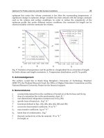
compared with measured heat flux values (see also (Vlasov et al., 2009)).




Fig. 1. Calculated distribution of non-dimensional heat flux Q = q/q
0
on the windward side
of the blunt delta wing. q
0

– heat flux at the stagnation point of a sphere with a radius equal
to the nose radius of the wing
Perfect gas hypersonic flow (γ = 1.4) past a delta wing with a spherical nose and cylindrical
edges of the same radius is considered. Mach and Reynolds numbers calculated with free
stream flow parameters and the wing nose radius are M
∞
= 14 and Re
∞
= 1.4·10
4
, angle of
attack α = 10°, wing sweep angle λ = 75°. The free stream stagnation temperature
T
0∞
= 1205 K, the wall temperature T
w
= 300 K. Due to the symmetry of flow, only half of the
wing is computed. The flow calculation was performed with shock-fitting procedure, the
computational grid is 120×40×119 (in the longitudinal, transverse and circumferential
Heat Transfer - Mathematical Modelling, Numerical Methods and Information Technology

240
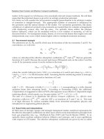
directions, respectively, see Fig. 2). Below in this section all quantities with a dimension of
length, unless otherwise specified, are normalized to the wing nose radius r.


Fig. 2. The computational grid on the wing surface, in the plane of symmetry (z = 0) and in
the exit section for the converged numerical solution

Fig. 3. Streamlines near the windward surface of the wing. Top – at a distance of one grid
step from the wall, bottom – at the outer edge of the boundary layer
Calculated patterns of streamlines near the windward surface of the wing at a distance of
one grid step from the wall and at the outer edge of the boundary layer are shown in Fig. 3.
The streamlines, flowing down from the wing edge on the windward plane at almost
constant pressure, form the line of diverging flow (line
A-A'), along which there are bands
of elevated heat fluxes. At the symmetry plane a line of converging streamlines is realized
along the entire length of the wing, but upstream the shock interaction point
A flow
impinges on the symmetry plane from the edges, and downstream from
A – from the
diverging line
A-A'. A characteristic feature of the considered case is that the distribution of
heat fluxes on the windward side is mainly determined by the values of convergence and
divergence of streamlines at almost constant pressure (see Fig. 4, which shows the
distribution of pressure and heat flux on the windward side in several sections x = const).
Local maxima of heat fluxes near symmetry plane appear only at x> 15 near the line z = 4
(after the nose shock wave intersects with the shock wave from the edges) and the relative
intensity of these heat peaks grows with increasing distance from the nose (Fig. 4b).
Aerodynamic Heating at Hypersonic Speed

241
0.03
0.08
00.51
P
1
23

4
5
z*
0
0.05
0.1
0.15
0510
Q
z
1
2
3
4

(a) (b)
Fig. 4. Pressure distribution Р = p/ρ
∞
V
∞
2
(a) and heat flux Q = q/q
0
(b) on windward side of
wing in sections: 1-5 – x = 10, 20, 30, 50, 90, z*= z/z
max
, z
max
– wingspan in section х = const
Comparison of the upper and lower parts of Fig. 3 shows that the flow near the wall and at

the outer edge of the boundary layer are noticeably different, the streamlines near the wall
are directed to the symmetry plane (converging), and in inviscid region – from it
(diverging). It follows that the velocity component directed along the wing chord changes
sign across the boundary layer, which indicates the existence of transverse vortex (cross
separation flow) in the boundary layer. This is illustrated in Fig. 5a, which shows the
projection of streamlines on the plane of the cross section at x = 90.


4
0
0
1
2
0
0
1
2
0
0
7
0
0
1
0
0
0
T
0

(a) (b)

Fig. 5. Projection of streamlines (a) and isolines of stagnation temperature T
0
, K (b) in cross
section x = 90
The distribution of the boundary layer thickness is clearly seen in Fig. 5b, which shows the
contours of the stagnation temperature T
0
in the cross section x = 90. On the windward side
of the wing minimum thickness of the boundary layer is located on the diverging line (line
A-A' in Fig. 3). On the left and on the right sides of the diverging line there are converging
lines with a thicker boundary layer (about 2 and 3 times respectively). One of the
Heat Transfer - Mathematical Modelling, Numerical Methods and Information Technology

242
converging lines is the symmetry plane. Here the boundary layer thickness on the
windward side reaches a maximum, amounting to about one-third of the shock layer
thickness.
Near the wing edge because of the expansion and acceleration of the flow the boundary
layer thickness decreases sharply (at the edge it is almost 20 times less than at the symmetry
plane on the windward side). On the leeward side of the wing flow separation occurs, and
the concept of the boundary layer loses its meaning. Here scope of viscous flow is half the
shock layer.
The shape of calculated shock wave in Fig. 6a, induced by the wing nose as a blunt body, is
determined by the law of the explosive analogy, so that some front part of the wing
x
≤
x
A
≈ 15 will be located inside the initially axisymmetric shock wave. The coordinate of
point

A (x
A
) is located in the vicinity of interaction region of shock waves induced by the
nose and the edges of the wing. Here the profiles of pressure and heat flux along the edge
are local maxima.

0
10
0.00
0.05
01530
z
P
Q/2
x
shock
wing edge
P
Q
x
A
0
0.05
-1 -0.5 0 0.5 1
Q
z*
calculation
experiment

(a) (b)

Fig. 6. Profiles of pressure, heat flux and the shock wave along the wing edge (a) and
distribution of heat fluxes in cross section x = 90 (b)
In Fig. 6b the distribution of computed heat fluxes q/q
0
in the neighborhood of the wing end
section at x = 90 is presented in comparison with the experiment of Gubanova et al. (1992)
depending on the transverse coordinate z. On the whole the calculation correctly predicts
the magnitude and position of local maximum of heat flux near the symmetry plane, taking
into account the small asymmetry in the experimental data. Note that near the minima of
heat fluxes calculated values are lower than experimental ones, probably due to effect of
smoothing of experimental data in these narrow regions.
3.2 Heat transfer on test model of Pre-X space vehicle
Currently developed hypersonic aircraft have dimensions several times smaller than
previously created space vehicles "Shuttle" and "Buran". This results in increase of heat load
on a vehicle during flight, and therefore the problem of reliable calculation of heat fluxes on
the surface for such relatively small bodies is particularly important. Thus the problem
arises of verification of the employed physical models and numerical methods by
comparing calculation results with experimental data.
Aerodynamic Heating at Hypersonic Speed

243
In 2006-2007 on TsNIImash’s experimental base in a piston gasdynamic wind tunnel PGU-7
a heat transfer study has been conducted on a small-scale model of Pre-X reentry
demonstrator (Baiocco, 2006). This vehicle is designed to obtain in flight conditions
experimental data pertaining to aerothermodynamic phenomena that are not modeled in
ground tests, but they are critical for design of a vehicle returning from the Earth’s orbit. In
particular, Pre-X demonstrator is developed to test in a real flight and in specified locations
on the vehicle surface samples of reusable thermal protection materials and to assess their
durability.
During the study thermovision measurements have been conducted of heat fluxes on the

model of scale 1/15 at various flow regimes – M = 10, Re = 1·10
6
-5·10
6
1/m (Kovalev et al.,
2009). Processing of thermovision measurements was carried out in accordance with
standard technique and composed of determination of the model surface temperature
during experiment, extraction from these data distributions of heat fluxes on the observed
model surface and binding of the resulting thermovision frame to a three-dimensional CAD
model of the demonstrator. The same CAD model has been used for numerical simulation of
heat transfer on the Pre-X test model.
As a normalizing value the heat flux q
0
at the stagnation point of a sphere with radius of
70 mm is adopted, which is determined using the Fay-Riddell formula. Advantage of data
presentation in this form is due to invariability of the relative values Q = q/q
0
on most
model surface at variations of flow parameters.



Fig. 7. Calculated distributions of pressure Р = р/ρ
∞
V
∞
2
(left) and stagnation temperature T
0
,

K (right) on surface and in shock layer (in symmetry plane and in exit section) for test model
of Pre-X vehicle
On the base of the numerical solution of the Navier-Stokes equations a study was carried
out of flow parameters and heat transfer for laminar flow over a test model of Pre-X space
Heat Transfer - Mathematical Modelling, Numerical Methods and Information Technology

244
vehicle for experimental conditions in the piston gasdynamic wind tunnel. Mach and
Reynolds numbers, calculated from the free-stream parameters and the length of the model
(330 mm), are M
∞
= 10 and Re
∞
= 7·10
5
. Angle of attack – 45°. The flap deflection angle was
(as in the experiment) δ = 5, 10 and 15°. The stagnation temperature of the free-stream flow
and the wing surface temperature – T
0∞
= 1000 K and T
w
= 300 K, respectively. An
approximation of a perfect gas was used with ratio of specific heats γ = 1.4. The calculations
were performed with a shock-fitting procedure, i.e. the bow shock was considered as a
discontinuity with implementation of the Rankine-Hugoniot relations (4) across it. On the
model surface no-slip and fixed temperature conditions were set. Note that in view of the
flow symmetry computations were made only for a half of the model, although in the
figures below for comparison with experiment the calculated data (upon reflection in the
symmetry plane) are presented on the entire model.
The overall flow pattern obtained in the calculations over the test model of Pre-X space

vehicle is shown in Fig. 7, where for the case of the flap deflection angle δ = 15° pressure and
stagnation temperature Т
0
isolines in the shock layer and on the model surface are shown. It
is seen that there are two areas of high pressure: on the nose tip of the model (P ≈ 0.92) and
on the deflection flaps. In the latter case the pressure in the flow passing through the two
shock waves reaches P ≈ 1.3. Isolines of Т
0
show the size of regions where viscous forces are
significant: a thin boundary layer on the windward side of the model and an extensive
separation zone on the leeward side. The small separation zone, appearing at deflection
flaps, although about four times thicker than the boundary layer upstream of it is almost not
visible in the scale of the figure.
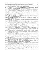
Fig. 8 shows the distributions of relative heat flow Q on the windward side of the model
obtained in the experiments and in the calculations at deflection angles of flaps δ = 5, 10 and
15°. For the case δ = 5° it can be noted rather good agreement between experiment and
calculation in the values of heat flux in the central part of the model and on the flaps. It is
evident that before deflected flaps there is a region of low heat fluxes caused by near
separation state (according to calculation results) of the boundary layer.
In analyzing the experimental data it should be taken into account the effect of "apparent"
temperature reduction of the surface area with a large angle to the thermovision observation
line. It is precisely this effect that explains the fact that in the nose part of the model the
experimental values of heat flux are less than the calculated ones. Also narrow zones of high
(at the sharp edges of the flaps) or low (in the separation zone at the root of the flaps) values
of heat flux are smoothed or not visible in the experiment due to insufficient resolution of
thermovision equipment. The resolution capability of thermovisor is clearly visible by the
size of cells in the experimental isoline pattern of heat flux in Fig. 8. It should be noted that
the calculations do not take into account a slit between the deflection flaps available on the
test model, the presence of which should lead to a decrease in the separation region in front
of the flaps.

At an angle of flap deflection δ = 10°, as in the previous case δ = 5°, there is fairly good
agreement between calculation and experiment for the values of heat flux in the central part
of the model and on the flaps. The calculations show that the growth of the flap deflection
angle δ from 5° to 10° results in the formation of a large separation zone in front of the flaps
and in a decrease in heat flux value Q from 0.2 to 0.1.
At the largest angle of flap deflection δ = 15° the maximum of calculated heat flux occurs in
the zone of impingement of the separated boundary layer, where the level of Q is 2-3 times
higher than its level on the undeflected flap. The coincidence of calculation results with
Aerodynamic Heating at Hypersonic Speed

245
experimental data in the front part of the model up to the separation zone before the flaps is
satisfactory. On the flaps the level of heat flux in the experiment is about one and a half
times more than in the calculation. This difference in heat flux values is apparently due to
laminar-turbulent transition in separation region induced by the deflected flaps which takes
place in the experiment.


δ= 5°



δ = 10
°


δ = 15
°

Fig. 8. Experimental (left) and calculated (right) heat fluxes Q = q/q

0
on windward side of
test model of Pre-X space vehicle at different deflection angles of flaps δ.
Heat Transfer - Mathematical Modelling, Numerical Methods and Information Technology

246
3.3 Flow and heat transfer on a winged space vehicle at reentry to Earth's atmosphere
This section presents the results of numerical simulation of flow and heat transfer on a
winged version of the small-scale reentry vehicle, being developed in TsAGI (Vaganov et al,
2006), moving at hypersonic speed in the Earth's atmosphere. Calculations were made using
two physical-chemical models of the gas medium - equilibrium and non-equilibrium
chemically reacting air.
The bow shock was captured in contrast to the previous two flow cases. Thus on the inflow
boundary the free-stream conditions were specified. On the vehicle surface no-slip and
adiabatic wall conditions were supposed. In calculations with use of the nonequilibrium air
model the vehicle surface was supposed to be low catalytical with the probability of
heterogeneous recombination of O and N atoms equal to γ
А
= 0.01.
A computational grid was provided by Mikhalin V.A. (Dmitriev et al., 2007), and was taken
from the inviscid flow calculation. The number of points in the direction normal to the
vehicle surface has been increased to resolve the wall boundary layer. Part of the results
presented below was reported in (Dmitriev et al., 2007; Gorshkov et al., 2008a).
Calculations were performed for two points of a reentry trajectory, for which thermal loads
are close to maximum (Table 1). The angle of attack α = 35°, the vehicle length L = 9m. A
grid 93×50×101 in the longitudinal, transverse and circumferential directions respectively
were used in the calculations. The surface grid of the vehicle is shown in Fig. 9.

Н,
km

V
∞
,
m/sec
Re
∞,L
M
∞

Р
∞
, atm Т
∞
, K
70 5952 3.46·10
5
20.0 5.76·10
-5
219
63 5152 6.84·10
5
16.6 1.59·10
-4
243
Table 1. Parameters of trajectory points


Fig. 9. Surface grid of the small-scale reentry vehicle
In Fig. 10a contours of total enthalpy H
0

on the surface and in the shock layer near the
reentry vehicle are shown. On the windward side one can see the shock wave, the thin wall
boundary layer and the inviscid flow between them, in which the values of H
0
are constant.
In the calculations the shock wave is smeared upon 3-5 grid points and has a finite thickness
due to the use of artificial dissipation. In particular, a local decrease in H
0
in a strong shock
Aerodynamic Heating at Hypersonic Speed

247
wave on the windward side, which can be seen in the figure, has no physical meaning and is
due to the influence of artificial dissipation. Recall that the Navier-Stokes equations do not
correctly describe the shock structure at Mach numbers M> 1.5.
In the shock layer on the leeward side it is visible a large area with reduced values of total
enthalpy Н
0
<Н
0∞
(Н
0∞
– total enthalpy in the free-stream), which arises as a result of
boundary layer separation from the vehicle surface.
Chemical processes occurring in the shock layer over the vehicle are illustrated in Fig. 10b,
which shows contours of mass concentrations of oxygen atoms с
о
. Under the considered
conditions in the vicinity of the vehicle nose behind the shock wave O
2

dissociation is
complete. On the windward side downstream the nose in the shock layer and on the surface
the recombination occurs and the concentration of O decreases. In contrast, on the leeward
side where the flow is very rarefied, the level of с
о
remains high, indicating that the process
of recombination of atomic oxygen is frozen.


boundar
y
la
y
er
shock wave

(a) (b)
Fig. 10. Total enthalpy, MJ/kg (a), and mass concentration of oxygen atoms (b) on the
surface and in the shock layer near the vehicle. Н = 63 km


0.001
0.01
0.1
1
0510
P
x, m
equilibrium air
nonequilibrium air

equilibrium air

Fig. 11. Pressure distribution P = р/ρ
∞
V
∞
2
on vehicle surface, overall view (left) and in
symmetry plane (right), Н = 63 km
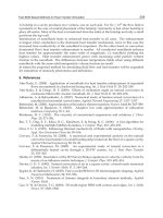
Heat Transfer - Mathematical Modelling, Numerical Methods and Information Technology

248
In Fig. 11 and 12 isolines of pressure, heat flux q
w
and equilibrium radiation temperature T
w

on the vehicle surface are shown for cases of equilibrium and non-equilibrium dissociating
air. Comparison of q
w
and T
w
distributions on the vehicle surface in the symmetry plane for
two air models are depicted in Fig. 13.
Analysis of the calculation results shows that pressure distribution on the windward surface
of the vehicle does not depend on physical-chemical model of the gas medium - the
difference in pressure values for equilibrium and non-equilibrium air flow is 1 - 2%. On the
leeward side pressure on the surface for nonequilibrium flow may be nearly two times

lower than for equilibrium flow (e.g., in the vicinity of the tail). This is probably due to the
fact that the effective ratio of specific heats for nonequilibrium air is greater than for
equilibrium air, because in the shock layer on the leeward side nonequilibrium flow is
chemically frozen, and here there is a sufficiently high concentration of atoms (see Fig. 10b).




equilibrium air
nonequilibrium air

Fig. 12. Distributions of heat flux q
w
, kW/m
2
, (top) and equilibrium radiation temperature
T
w
,°C, (bottom) on the vehicle surface, Н = 63 km
Nonequilibrium chemical processes in the shock layer and finite catalytic activity of the
vehicle surface (γ
А
= 0.01) significantly reduce the calculated levels of heat transfer in
comparison with the case of equilibrium air flow. The most significant decrease in heat flux
is observed on the vehicle nose part (for x ≤ 1 m) and in the vicinity of the tail. For example,
at the nose stagnation point the level of heat flux decreases by about 40% – from 640 to 385
kW/m
2
, while the surface temperature decreases by nearly 15% – from 1670 to 1430 °C.
Note a high heat flux level on the thin edge of the wing compared with one at the nose

stagnation point. Particularly intense heating occurs at the sharp bend of the wing where the
values of heat flux and surface temperature even slightly exceed their values at the front
stagnation point. In the case of equilibrium air flow the exceeding for heat flux is about 10%
(710 and 640 kW/m
2
), for temperature - 3% (1720 and 1670 °C). In the case of
nonequilibrium air flow the exceeding is more significant, for heat flux - 30% (540 and 385
kW/m
2
), for temperature - 10% (1570 and 1430 ° C).
Aerodynamic Heating at Hypersonic Speed

249
In other parts of the vehicle surface difference in heat flux levels for the two air models is
somewhat less, and it decreases downstream, presumably due to gradual recombination of
atoms in the boundary layer at flowing along the surface in case of non-equilibrium air.


1
10
100
1000
0510
Q
w
x, m
equilibrium air
nonequilibrium air
0
1000

2000
0510
T
w
x, m
equilibrium air
nonequilibrium air


Fig. 13. Profiles of heat flux q
w
, kW/m
2
, (left) and equilibrium radiation temperature T
w
,°C,
(right) on vehicle surface in symmetry plane, Н = 63 km
A similar flow and heat flux patterns are observed for the altitude H = 70 km, as seen in
Fig. 14 where contours of heat flux and equilibrium radiation wall temperature are shown at
this altitude for the two air models. For equilibrium air overall level of heat flux at 70 km is
slightly higher than at 63 km. For example heat flux value at the nose stagnation point is
increased by 5% (675 compared with 640 kW/m
2
). The opposite situation occurs for the
model of nonequilibrium air, in this case the stagnation point heat flux value at 70 km is
lower than at 63 km – by 7% (360 and 385 kW/m
2
respectively).

equilibrium air
nonequilibrium air


Fig. 14. Distributions of heat flux q
w
, kW/m
2
, (top) and equilibrium radiation temperature
T
w
,°C, (bottom) on the vehicle surface, Н = 70 km
Heat Transfer - Mathematical Modelling, Numerical Methods and Information Technology

250
4. Conclusion
A three-dimensional stationary Navier–Stokes computer code for laminar flow, developed
by the author, has been briefly described. The code is mainly intended to calculate super-
and hypersonic flows over bodies accounting for high temperature real gas effects with
special emphasis on convective heat transfer. Three gas models: perfect gas, equilibrium and
nonequilibrium gas mixture can be used in the calculations.
In the chapter a comparison of code calculation results with experimental data is made for
two perfect gas hypersonic flow cases at wind tunnel conditions. First case is a simulation of
an anomalous heat transfer on the windward side a delta wing with blunt edges. On the
whole the calculation correctly predicts the magnitude and position of local maximum of
heat flux near the wing symmetry plane, taking into account a small asymmetry in the
experimental data. Second case is a computation of heat transfer on a test model of the Pre-X
demonstrator. Satisfactory agreement with thermovision heat fluxes on the smooth
windward side and on the flaps is obtained, except for the largest deflection angle of flaps
δ = 15° when the level of heat flux in the experiment is about one and a half times more than

in the calculation. This discrepancy is apparently due to laminar-turbulent transition in
separation region induced by the deflected flaps which takes place in the experiment.
Third flow case concerns chemically reacting air flow at equilibrium or nonequilibrium
conditions. Flowfield and convective heat transfer parameters for a winged shape of a small-
scale reentry vehicle are calculated for two points of a reentry trajectory in the Earth’s
atmosphere. Heat flux and equilibrium radiation temperature distributions on the vehicle
surface are obtained. Also regions of maximal thermal loadings are localized.
Calculations show that for nonequilibrium air flow the use of a low catalytic coating (with
probability of heterogeneous recombination of atoms γ
А
= 0.01) on the vehicle surface
enables to decrease considerably the level of heat fluxes in regions of maximal heat transfer
in the nose part and on the wing edges in comparison with equilibrium air flow. For
example for trajectory points with maximal thermal load a reduction of up to 40% in heat
flux (which results in a 15% reduction of equilibrium radiation wall temperature) can be
obtained at the vehicle nose.
5. Acknowledgments
The author is grateful to Kovalev R.V., Marinin V.P. and Vlasov V.I. for delivering
thermovision data on test model of Pre-X vehicle, and also to Churakov D.A. and Mihalin
V.A. for providing computational grids.
6. References
Baiocco, P.; Guedron, S.; Plotard, P. & Moulin, J. (2006). The Pre-X atmospheric re-entry
experimental lifting body: Program status and system synthesis, Proceedings of 57th
International Astronautical Congress, 2-6 October 2006. IAC-06-D2.P.2.2
Churakov, D.A.; Gorshkov, A.B.; Kovalev, R.V.; Vlasov, V.I.; Beloshitsky, A.V.; Dyadkin,
A.A. & Zhurin, S.V. (2008). Heat Transfer of Reentry Vehicles during Atmosphere
Flight, Proceedings of 6-th European Symposium on Aerothermodynamics for Space
Vehicles, Versailles, France, 3 - 6 November 2008.
Aerodynamic Heating at Hypersonic Speed

251
Dmitriev, V.G.; Vaganov, A.V.; Gorshkov, A.B.; Lapygin, V.I.; Galaktionov, A.Yu. &
Mikhalin, V.A. (2007). Analysis of Aerothermodynamic Parameters of Reusable
Space Wing Vehicle, Proceedings of 2nd European Conference for Aero-Space Sciences,
Brussels, Belgium, July 1-6 2007
Gorshkov A.B. (1997) Calculation of Base Heat Transfer Behind Thin Cone-Shaped Bodies.
Cosmonautics and Rocket Engineering, No. 11, (1997) pp. 13-20 (in Russian)
Gorshkov, A.B.; Kovalev, R. V.; Vlasov, V. I. & Zemlyanskiy, B. A. (2008a). Simulation of
Heat Transfer to Space Vehicles during a Gliding Reentry into Earth’s
Atmosphere, Proceedings of 14th International Conference on Methods of Aerophysical
Research (ICMAR-2008), Novosibirsk, Russia, 30 June - 06 July 2008
Gorshkov, A.B.; Kovalev, R. V.; Vlasov & V. I., Zemlyanskiy, B. A. (2008b). Heat Transfer
Investigation for Hypersonic Flow over Experimental Model of Pre-X Reentry
Vehicle, Proceedings of 7th Sino-Russian High-Speed Flow Conference (SRHFC-7),
Novosibirsk, Russia, 1 - 3 July 2008
Grantham W.L. (1970). Flight results of a 25,000 fps re-entry experiment, NASA TN D 6062.
Gubanova, O.I.; Zemlyansky, B.A.; Lessin, A.B.; Lunev, V.V.; Nikulin, A.N. & Syusin A.V.
(1992). Anomalous heat transfer on the windward side of a delta wing with a blunt
tip in hypersonic flow, In: Aerothermodynamics of aerospace systems, Pt. 1, pp. 188-196,
Moscow, TsAGI (in Russian)
Hoffmann, K.A.; Chiang, S.T. (2000). Computational fluid dynamics, Vol. 2, Engineering
Educational Systems, ISBN 0-9623731-3-3, Kansas, USA
Inouye, Y. (1995). OREX flight – quick report and lessons learned. Proceedings of 2nd
European Symposium on Aerothermodynamics for Space Vehicles, pp. 271-279, ESTEC,
Noordwik, The Netherlands, Europe Space Agency (November 1994).
Kovalev, R.V.; Kislykh, V.V.; Kolozezniy, A.E.; Kudryavtsev, V.V.; Marinin, V.P.; Vlasov,
V.I. & Zemliansky, B.A. (2009). Experimental studies of Pre-X vehicle heat transfer
in PGU-7 test facility, 3rd European Conference for Aerospace Sciences (EUCASS-2009),
Versailles, France, 6-9 July 2009
Lesin, A.B. & Lunev, V.V. (1994). Heat transfer peaks on a blunt-nosed triangular plate in

hypersonic flow. Fluid Dynamics, Vol. 29, No. 2, (April 1994) pp. 258-262, ISSN:
0015-4628
Mason, E.A. & Saxena, S.C. (1958). Approximate Formula for the Thermal Conductivity of
Gas Mixtures. Phys. Fluids, Vol. 1, No. 5, (1958) pp. 361-369
Pulliam, T.H. (1986). Artificial dissipation models for the Euler equations. AIAA Journal,
Vol.24, No. 12, (December 1986) pp. 1931-1940, ISSN: 0001-1452
Vaganov, A.V.; Dmitriev, V.G.; Zadonsky, S.M.; Kireev, A.Y.; Skuratov, A.S. & Stepanov,
E.A. (2006). Estimations of low-sized winged reentry vehicle heat regimes on the
stage of its designing. Physico-chemical kinetics in gas dynamics,
www.chemphys.edu.ru/pdf/2006-11-20-002.pdf (in Russian)
Vlasov, V.I.; Gorshkov, A.B.; Kovalev, R.V. & Plastinin, Yu.A. (1997). Theoretical studies of
air ionization and NO vibrational excitation in low density hypersonic flow around
re-entry bodies. AIAA Paper
. No. 97-2582 (1997)
Vlasov, V. I. & Gorshkov, A. B. (2001). Comparison of the Calculated Results for Hypersonic
Flow Past Blunt Bodies with the OREX Flight Test Data. Fluid Dynamics, Vol. 36,
No 5, (October 2001) pp. 812-819, ISSN: 0015-4628
Heat Transfer - Mathematical Modelling, Numerical Methods and Information Technology

252
Vlasov, V.I.; Gorshkov, A.B.; Kovalev, R.V. & Lunev, V.V. (2009). Thin triangular blunt-
nosed plate in a viscous hypersonic flow. Fluid Dynamics, Vol. 44, No. 4 (August
2009) pp. 596-605, ISSN: 0015-4628
Wilke, C. (1950). A Viscosity Equation for Gas Mixtures. J.Chem.Phys., Vol. 18, No. 4, (1950)
pp.517-519
Yoon, S. & Jameson, A. (1987). An LU-SSOR Scheme for the Euler and Navier-Stokes
Equations. AIAA Paper. No. 87-0600 (1987)
11
Thermoelastic Stresses in FG-Cylinders
Mohammad Azadi

1
and Mahboobeh Azadi
2

1
Department of Mechanical Engineering, Sharif University of Technology
2
Department of Material Engineering, Tarbiat Modares University
Islamic Republic of Iran
1. Introduction
FGM components are generally constructed to sustain elevated temperatures and severe
temperature gradients. Low thermal conductivity, low coefficient of thermal expansion
and core ductility have enabled the FGM material to withstand higher temperature
gradients for a given heat flux. Examples of structures undergo extremely high
temperature gradients are plasma facing materials, propulsion system of planes, cutting
tools, engine exhaust liners, aerospace skin structures, incinerator linings, thermal barrier
coatings of turbine blades, thermal resistant tiles, and directional heat flux materials.
Continuously varying the volume fraction of the mixture in the FGM materials eliminates
the interface problems and mitigating thermal stress concentrations and causes a more
smooth stress distribution.
Extensive thermal stress studies made by Noda reveal that the weakness of the fiber rein-
forced laminated composite materials, such as delamination, huge residual stress, and
locally large plastic deformations, may be avoided or reduced in FGM materials (Noda,
1991). Tanigawa presented an extensive review that covered a wide range of topics from
thermo-elastic to thermo-inelastic problems. He compiled a comprehensive list of papers on
the analytical models of thermo-elastic behavior of FGM (Tanigawa, 1995). The analytical
solution for the stresses of FGM in the one-dimensional case for spheres and cylinders are
given by Lutz and Zimmerman (Lutz & Zimmerman, 1996 & 1999). These authors consider
the non-homogeneous material properties as linear functions of radius. Obata presented the
solution for thermal stresses of a thick hollow cylinder, under a two-dimensional transient

temperature distribution, made of FGM (Obata et al., 1999). Sutradhar presented a Laplace
transform Galerkin BEM for 3-D transient heat conduction analysis by using the Green's
function approach where an exponential law for the FGMs was used (Sutradhar et al., 2002).
Kim and Noda studied the unsteady-state thermal stress of FGM circular hollow cylinders
by using of Green's function method (Kim & Noda, 2002). Reddy and co-workers carried out
theoretical as well as finite element analyses of the thermo-mechanical behavior of FGM
cylinders, plates and shells. Geometric non-linearity and effect of coupling item was
considered for different thermal loading conditions (Praveen & Reddy, 1998, Reddy & Chin,
1998, Paraveen et al., 1999, Reddy, 2000, Reddy & Cheng, 2001). Shao and Wang studied the
thermo-mechanical stresses of FGM hollow cylinders and cylindrical panels with the
assumption that the material properties of FGM followed simple laws, e.g., exponential law,