Heat Transfer Mathematical Modelling Numerical Methods and Information Technology Part 1 pptx

HEAT TRANSFER ͳ
MATHEMATICAL
MODELLING,
NUMERICAL METHODS
AND INFORMATION
TECHNOLOGY
Edited by Aziz Belmiloudi
Heat Transfer - Mathematical Modelling,
Numerical Methods and Information Technology
Edited by Aziz Belmiloudi
Published by InTech
Janeza Trdine 9, 51000 Rijeka, Croatia
Copyright © 2011 InTech
All chapters are Open Access articles distributed under the Creative Commons
Non Commercial Share Alike Attribution 3.0 license, which permits to copy,
distribute, transmit, and adapt the work in any medium, so long as the original
work is properly cited. After this work has been published by InTech, authors
have the right to republish it, in whole or part, in any publication of which they
are the author, and to make other personal use of the work. Any republication,
referencing or personal use of the work must explicitly identify the original source.
Statements and opinions expressed in the chapters are these of the individual contributors
and not necessarily those of the editors or publisher. No responsibility is accepted
for the accuracy of information contained in the published articles. The publisher
assumes no responsibility for any damage or injury to persons or property arising out
of the use of any materials, instructions, methods or ideas contained in the book.

Publishing Process Manager Iva Lipovic
Technical Editor Teodora Smiljanic
Cover Designer Martina Sirotic
Image Copyright Zadiraka Evgenii, 2010. Used under license from Shutterstock.com
First published February, 2011

Printed in India
A free online edition of this book is available at www.intechopen.com
Additional hard copies can be obtained from
Heat Transfer - Mathematical Modelling, Numerical Methods and
Information Technology, Edited by Aziz Belmiloudi
p. cm.
ISBN 978-953-307-550-1
free online editions of InTech
Books and Journals can be found at
www.intechopen.com

Part 1
Chapter 1
Chapter 2
Chapter 3
Chapter 4
Part 2
Chapter 5
Chapter 6
Chapter 7
Chapter 8
Preface IX
Inverse, Stabilization and Optimization Problems 1
Optimum Fin Profile under Dry
and Wet Surface Conditions 3
Balaram Kundu and Somchai Wongwises
Thermal Therapy: Stabilization and Identification 33
Aziz Belmiloudi
Direct and Inverse Heat Transfer Problems
in Dynamics of Plate Fin and Tube Heat Exchangers 77

Dawid Taler
Radiative Heat Transfer
and Effective Transport Coefficients 101
Thomas Christen, Frank Kassubek, and Rudolf Gati
Numerical Methods and Calculations 127
Finite Volume Method Analysis of Heat Transfer
in Multi-Block Grid During Solidification 129
Eliseu Monteiro, Regina Almeida and Abel Rouboa
Lattice Boltzmann Numerical Approach
to Predict Macroscale Thermal Fluid Flow Problem 151
Nor Azwadi Che Sidik and Syahrullail Samion
Efficient Simulation of Transient Heat
Transfer Problems in Civil Engineering 165
Sebastian Bindick, Benjamin Ahrenholz, Manfred Krafczyk
Applications of Nonstandard Finite Difference
Methods to Nonlinear Heat Transfer Problems 185
Alaeddin Malek
Contents
Contents
VI
Fast BEM Based Methods
for Heat Transfer Simulation 209
Jure Ravnik and Leopold Škerget
Aerodynamic Heating at Hypersonic Speed 233
Andrey B. Gorshkov
Thermoelastic Stresses in FG-Cylinders 253
Mohammad Azadi and Mahboobeh Azadi
Experimentally Validated Numerical Modeling
of Heat Transfer in Granular Flow in Rotating Vessels 271
Bodhisattwa Chaudhuri, Fernando J. Muzzio

and M. Silvina Tomassone
Heat Transfer in Mini/Micro Systems 303
Introduction to Nanoscale Thermal Conduction 305
Patrick E. Hopkins and John C. Duda
Study of Hydrodynamics and Heat
Transfer in the Fluidized Bed Reactors 331
Mahdi Hamzehei
Particle Scale Simulation
of Heat Transfer in Fluid Bed Reactors 383
Zongyan Zhou, Qinfu Hou and Aibing Yu
Population Balance Model of Heat Transfer
in Gas-Solid Processing Systems 409
Béla G. Lakatos
Synthetic Jet-based Hybrid Heat Sink
for Electronic Cooling 435
Tilak T Chandratilleke, D Jagannatha and R Narayanaswamy
Turbulent Flow and Heat Transfer
Characteristics of a Micro Combustor 455
Tae Seon Park and Hang Seok Choi
Natural Circulation in Single
and Two Phase Thermosyphon Loop
with Conventional Tubes and Minichannels 475
Henryk Bieliński and Jarosław Mikielewicz
Heat Transfer at Microscale 497
Mohammad Hassan Saidi and Arman Sadeghi
Chapter 9
Chapter 10
Chapter 11
Chapter 12
Part 3

Chapter 13
Chapter 14
Chapter 15

Chapter 16
Chapter 17
Chapter 18
Chapter 19
Chapter 20
Contents
VII
Energy Transfer and Solid Materials 527
Thermal Characterization of Solid Structures
during Forced Convection Heating 529
Balázs Illés and Gábor Harsányi
Analysis of the Conjugate Heat Transfer
in a Multi-Layer Wall Including an Air Layer 553
Armando Gallegos M., Christian Violante C.,
José A. Balderas B., Víctor H. Rangel H. and José M. Belman F.
An Analytical Solution for Transient Heat
and Moisture Diffusion in a Double-Layer Plate 567
Ryoichi Chiba
Frictional Heating in the Strip-Foundation Tribosystem 579
Aleksander Yevtushenko and Michal Kuciej
Convective Heat Transfer Coefficients
for Solar Chimney Power Plant Collectors 607
Marco Aurélio dos Santos Bernardes
Thermal Aspects of Solar Air Collector 621
Ehsan Mohseni Languri and Davood Domairry Ganji
Heat Transfer in Porous Media 631

Ehsan Mohseni Languri and Davood Domairry Ganji
Part 4
Chapter 21
Chapter 22
Chapter 23
Chapter 24
Chapter 25
Chapter 26
Chapter 27

Pref ac e
During the last years, spectacular progress has been made in all aspects of heat trans-
fer. Heat transfer is a branch of engineering science and technology that deals with the
analysis of the rate of transfer thermal energy. Its fundamental modes are conduction,
convection, radiation, convection vs. conduction and mass transfer. It has a broad ap-
plication to many diff erent branches of science, technology and industry, ranging from
biological, medical and chemical systems, to common practice of thermal engineer-
ing (e.g. residential and commercial buildings, common household appliances, etc),
industrial and manufacturing processes, electronic devices, thermal energy storage,
and agriculture and food process. In engineering practice, an understanding of the
mechanisms of heat transfer is becoming increasingly important, since heat transfer
plays a crucial role in the solar collector, power plants, thermal informatics, cooling
of electronic equipment, refrigeration and freezing of foods, technologies for produc-
ing textiles, buildings and bridges, among other things. Engineers and scientists must
have a strong basic knowledge in mathematical modelling, theoretical analysis, experi-
mental investigations, industrial systems and information technology with the ability
to quickly solve challenging problems by developing and using new, more powerful
computational tools, in conjunction with experiments, to investigate design, paramet-
ric study, performance and optimization of real-world thermal systems.
In this book entitled ”Heat transfer - Mathematical Modelling, Numerical Methods

and Information Technology”, the authors provide a useful treatise on the principal
concepts, new trends and advances in technologies, and practical design engineering
aspects of heat transfer, pertaining to powerful tools that are modelling, computation-
al methodologies, simulation and information technology. These tools have become
essential elements in engineering practice for solving problems. The present book con-
tains a large number of studies in both fundamental and application approaches with
various modern engineering applications.
These include ”Inverse, Stabilization and Optimization Problems” (chapters 1 to 4),
which focus on modelling, stabilization, identification and shape optimization, with
application to biomedical processes, electric arc radiation and heat exchanger sys-
tems; ”Numerical Methods and Calculations” (chapters 5 to 12), which concern finite-
diff erence, finite-element and finite-volume methods, la ice Boltzmann numerical
method, nonstandard finite diff erence methods, boundary element method and fast
X
Preface
multipole method, quadrature scheme and complex geometries, hermitian transfinite
element, and numerical simulation with various applications as solidification, hy-
personic speed, concert hall, porous media and nanofluids; ”Heat Transfer in Mini/
Micro Systems” (chapters 13 to 20) which cover miniscale and microscale processes
with various applications such as fluidized beds reactors, flows conveying bubbles and
particles, microchannel heat sinks, micro heat exchangers, micro combustors and semi-
conductors; ”Energy Transfer and Solid Materials” (chapters 21 to 27) which concern
heat transfer in furnaces and enclosures, solid structures, moisture diff usion behav-
iour, porous media with various applications such as tribosystems and solar thermal
collectors.
The editor would like to express his thanks to all the authors for their contributions in
diff erent areas of their expertise. Their domain knowledge combined with their enthu-
siasm for scientific quality made the creation of this book possible.
The editor sincerely hopes that readers will find the present book interesting, valuable
and current.

Aziz Belmiloudi
European University of Bri any (UEB),
National Institut of Applied Sciences of Rennes (INSA),
Mathematical Research Institute of Rennes (IRMAR),
Rennes, France.


Part 1
Inverse, Stabilization and
Optimization Problems

1
Optimum Fin Profile under Dry and
Wet Surface Conditions
Balaram Kundu
1
and Somchai Wongwises
2
1
Department of Mechanical Engineering
Jadavpur University, Kolkata – 700 032
2
Fluid Mechanics, Thermal Engineering and Multiphase
Flow Research Lab (FUTURE), Department of Mechanical Engineering
King Mongkut’s University of Technology Thonburi (KMUTT)
Bangmod,Bangkok 10140

1
India
2

Thailand
1. Introduction
Fins or extended surfaces are frequently employed in heat exchangers for effectively
improving the overall heat transfer performance. The simple design of fins and their stability
in different surface conditions have created them a popular augmentation device. The different
fin shapes are available in the literature. The geometry of the fin may be dependent upon the
primary surface also. For circular primary surface, the attachment of circumferential fins is a
common choice. The longitudinal and pin fins are generally used to the flat primary surface.
However, due to attachment of fins with the primary surface, the heat transfer augments but
the volume, weight, and cost of the heat exchanger equipments increase as well. Hence, it is a
challenge to the designer to minimize the cost for the attachment of fins. This can be done by
determining the optimum shape of a fin satisfying the maximization of heat transfer rate for a
given fin volume. In general, two different approaches are considered for the optimization of
any fin design problem. Through a rigorous technique, the profile of a fin for a particular
geometry (flat or curved primary surface) may be obtained such that the criteria of the
maximum heat transfer for a given fin volume or equivalently minimum fin volume for a
given heat transfer duty is satisfied. In a parallel activity, the optimum dimensions of a fin of
given profile (rectangular, triangular etc.) are determined from the solution of the optimality
criteria. The resulting profile obtained from the first case of optimum design is superior in
respect to heat transfer rate per unit volume and thus it is very much important in fin design
problems. However, it may be limited to use in actual practice because the resulting profile
shape would be slightly difficult to manufacture and fabricate. Alternatively, such theoretical
shape would first be calculated and then a triangular profile approximating the base two
thirds of the fin would be used. Such a triangular fin transfers heat per unit weight, which is
closer to that of the analytical optimum value.
Under a convective environmental condition, Schmidt (1926) was the first researcher to
forward a systematic approach for the optimum design of fins. He proposed heuristically
that for an optimum shape of a cooling fin, the fin temperature must be a linear function
Heat Transfer - Mathematical Modelling, Numerical Methods and Information Technology

4
with the fin length. Later, through the calculus of variation, Duffin (1959) exhibited a
rigorous proof on the optimality criteria of Schmidt. Liu (1961) extended the variational
principle to find out the optimum profile of fins with internal heat generation. Liu (1962)
and Wilkins (1961) addressed for the optimization of radiating fins. Solov”ev (1968)
determined the optimum radiator fin profile. The performance parameter of annular fins of
different profiles subject to locally variable heat transfer coefficient had been investigated by
Mokheimer (2002). From the above literature works, it can be indicated that the above works
were formulated based on the “length of arc idealization (LAI).”
Maday (1974) was the first researcher to eliminate LAI and obtained the optimum profile
through a numerical integration. It is interesting to note that an optimum convecting fin
neither has a linear temperature profile nor possesses a concave parabolic shape suggested
by Maday. The profile shape contains a number of ripples denoted as a “wavy fin”. The
same exercise was carried out for radial fins by Guceri and Maday (1975). Later Razelos and
Imre (1983) applied Pontryagin's minimum principle to find out the minimum mass of
convective fins with variable heat transfer coefficient. Zubair et al. (1996) determined the
optimum dimensions of circular fins with variable profiles and temperature dependent
thermal conductivity. They found an increasing heat transfer rate through the optimum
profile fin by 20% as compare to the constant thickness fin.
A variational method was adopted by Kundu and Das (1998) to determine the optimum
shape of three types of fins namely the longitudinal fin, spine and disc fin. A generalized
approach of analysis based on a common form of differential equations and a set of
boundary conditions had been described. For all the fin geometries, it was shown that the
temperature gradient is constant and the excess temperature at the tip vanishes. By taking
into account the LAI, Hanin and Campo (2003) forecasted a shape of a straight cooling fin
for the minimum envelop. From the result, they have highlighted that the volume of the
optimum circular fin with consideration of LAI found is 6.21-8 times smaller than the
volume of the corresponding Schmidt’s parabolic optimum fin. A new methodological
determination for the optimum design of thin fins with uniform volumetric heat generation
had been done by Kundu and Das (2005).

There are ample of practical applications in which extended surface heat transfer is involved in
two-phase flow conditions. For example, when humid air encounter into a cold surface of
cooling coils whose temperature is maintained below the dew point temperature,
condensation of moisture will take place, and mass and heat transfer occur simultaneously.
The fin-and-tube heat exchangers are widely used in conventional air conditioning systems for
air cooling and dehumidifying. In the evaporator of air conditioning equipment, the fin surface
becomes dry, partially or fully wet depending upon the thermogeometric and psychrometric
conditions involved in the design process. If the temperature of the entire fin surface is lower
than the dew point of the surrounding air, there may occur both sensible and latent heat
transferred from the air to the fin and so the fin is fully wet. The fin is partially wet if the fin-
base temperature is below the dew point while fin-tip temperature is above the dew point of
the surrounding air. If the temperature of the entire fin surface is higher than the dew point,
only sensible heat is transferred and so the fin is fully dry. For wet surface, the moisture is
condensed on the fin surface, latent heat evolves and mass transfer occurs simultaneously with
the heat transfer. Thermal performance of different surface conditions of a fin depends on the
fin shape, thermophysical and psychrometric properties of air.
Many investigations have been devoted to analyze the effect of condensation on the
performance of different geometric fins. It is noteworthy to mention that for each instance, a
Optimum Fin Profile under Dry and Wet Surface Conditions

5
suitable fin geometry has been selected a priory to make the analysis. For the combined heat
and mass transfer, the mathematical formulation becomes complex to determine the overall
performance analysis of a wet fin. Based on the dry fin formula, Threlkeld (1970) and
McQuiston (1975) determined the one-dimensional fin efficiency of a rectangular longitudinal
fin for a fully wet surface condition. An analytical solution for the efficiency of a longitudinal
straight fin under dry, fully wet and partially wet surface conditions was introduced
elaborately by Wu and Bong (1994) first with considering temperature and humidity ratio
differences as the driving forces for heat and mass transfer. For the establishment of an
analytical solution, a linear relationship between humidity ratio and the corresponding

saturation temperature of air was taken. Later an extensive analytical works on the
performance and optimization analysis of wet fins was carried out by applying this linear
relationship. A technique to determine the performance and optimization of straight tapered
longitudinal fins subject to simultaneous heat and mass transfer has been established
analytically by Kundu (2002) and Kundu and Das (2004). The performance and optimum
dimensions of a new fin, namely, SRC profile subject to simultaneous heat and mass transfer
have been investigated by Kundu (2007a; 2009a). In his work, a comparative study has also
been made between rectangular and SRC profile fins when they are operated in wet
conditions. Hong and Web (1996) calculated the fin efficiency for wet and dry circular fins
with a constant thickness. Kundu and Barman (2010) have studied a design analysis of annular
fins under dehumidifying conditions with a polynomial relationship between humidity ratio
and saturation temperature by using differential transform method. In case of longitudinal fins
of rectangular geometry, approximate analytic solution for performances has been
demonstrated by Kundu (2009b). Kundu and Miyara (2009) have established an analytical
model for determination of the performance of a fin assembly under dehumidifying
conditions. Kundu et al. (2008) have described analytically to predict the fin performance of
longitudinal triangular fins subject to simultaneous heat and mass transfer.
The heat and mass transfer analysis for dehumidification of air on fin-and-tube heat
exchangers was done experimentally by the few authors. The different techniques, namely,
new reduction method, tinny circular fin method, finite circular fin method and review of
data reduction method used for analyzing the heat and mass transfer characteristics of wavy
fin-and-tube exchangers under dehumidifying conditions had been investigated by
Pirompugd et al. (2007a; 2007b; 2008; 2009).
The above investigations had been focused on determination of the optimum profile subjected
to convective environment. However a thorough research works have already been devoted
for analyzing the performance and optimization of wet fins. To carryout these analyses,
suitable fin geometry has been chosen a priory. However, the optimum profile fin may be
employed in air conditioning apparatus, especially, in aircrafts where reduction of weight is
always given an extra design attention. Kundu (2008) determined an optimum fin profile of
thin fins under dehumidifying condition of practical interest formulated with the treatment by

a calculus of variation. Recently, Kundu (2010) focused to determine the optimum fin profile
for both fully and partially wet longitudinal fins with a nonlinear saturation curve.
In this book chapter, a mathematical theory has been developed for obtaining the optimum fin
shape of three common types of fins, namely, longitudinal, spine and annular fins by
satisfying the maximizing heat transfer duty for a given either fin volume or both fin volume
and length. The analysis was formulated for the dry, partially and fully wet surface conditions.
For the analytical solution of a wet fin equation, a relationship between humidity ratio and
temperature of the saturation air is necessary and it is taken a linear variation. The influence of
Heat Transfer - Mathematical Modelling, Numerical Methods and Information Technology

6
wet fin surface conditions on the optimum profile shape and its dimensions has also been
examined. From the analysis, it can be mentioned that whether a surface is dry, partially or
fully wet at an optimum condition, the air relative humidity is a responsible factor. The
optimum fin profile and design variables have been determined as a function of thermo-
psychrometric parameters. The dry surface analysis can be possible from the present fully wet
surface fin analysis with considering zero value of latent heat of condensation. From the
analysis presented, it can be highlighted that unlike dry and partially wet fins, tip temperature
for fully wet fins is below the ambient temperature for the minimum profile envelop fin.
2. Variational formulations for the optimum fin shape
For determination of the optimum fin shape, it can be assumed that the condensate thermal
resistance to heat flow is negligibly small as the condensate film is much thinner than the
boundary layer in the dehumidification process. Under such circumstances, it may follow
that the heat transfer coefficient is not influenced significantly with the presence of
condensation. The condensation takes place when fin surface temperature is below the dew
point of the surrounding air and for its calculation, specific humidity of the saturated air on
the wet surface is assumed to be a linear function with the local fin temperature. This
assumption can be considered due to the smaller temperature range involved in the
practical application between fin base and dew point temperatures and within this small
range, saturation curve on the psychometric chart is possible to be an approximated by a

straight line (Wu and Bong, 1994; Kundu, 2002; Kundu, 2007a; Kundu, 2007b; Kundu, 2008;
Kundu, 2009). Owing to small temperature variation in the fin between fin-base and fin-tip,
it can be assumed that the thermal conductivity of the fin material is a constant. The
different types of fins, namely, longitudinal, spine and anuular fin are commonly used
according to the shape of the primary surfaces. Depending upon the fin base, fin tip and
dew point temperatures, fin-surface can be dry, partially and fully wet. The analysis for
determination of an optimum profile of fully and partially wet fins for longitudinal, spine
and annular fin geometries are described separately in the followings:
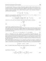
2.1 Fully wet longitudinal fins
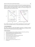
The schematic diagram of an optimum shape of longitudinal fins is illustrated in Fig. 1. The
governing energy equation for one-dimensional temperature distribution on fully wet
surface fins can be written under steady state condition as follows:

()( )
am afg
ddTh
y
TT h h h
dx dx k
ωω
⎛⎞
⎡
⎤
=−+−
⎜⎟
⎣
⎦
⎝⎠
(1)
h

m
is the average mass transfer coefficient based on the humidity ratio difference, ω is the
humidity ratio of saturated air at temperature T, ω
a
is the humidity ratio of the atmospheric
air, and h
jg
is the latent heat of condensation. For the mathematical simplicity, the following
dimensionless variables and parameters can be introduced:

Xhxk=
;
Yhyk=
;
Lhlk=
;
(
)
(
)
aab
TTTT
θ
=− −;
(
)
32
mp
Le h h C= (2)
where,

L
e
is the Lewis number. The relationship between heat and mass transfer coefficients
can be obtained from the Chilton-Colburn analogy (Chilton and Colburn, 1934). The
relationship between the saturated water film temperature T and the corresponding
Optimum Fin Profile under Dry and Wet Surface Conditions

7
saturated humidity ratio ω is approximated by a linear function (Wu and Bong, 1994;
Kundu, 2002; Kundu, 2007a; Kundu, 2007b; Kundu, 2008; Kundu, 2009) in this study:

abT
ω
=
+ (3)
where,
a and b are constants determined from the conditions of air at the fin base and fin tip.
Eq. (1) is written in dimensionless form by using Eqs. (2) and (3) as follows:










l
x

2y
b
1
2y
b
1
l
x
l
0
wet
dry
A
B

Fig. 1. Schematic diagram of an optimum longitudinal fin under dehumidifying conditions:
A. Fully wet; and B. Partially wet.

(
)
(
)
1ddXYd dX b
φ
ξφ
=+ (4)
where

p
φ

θθ
=+
;
(
)
(
)
(
)
1
pa a ab
abT T T b
θ
ωξ
⎡
⎤
=−− − +
⎣
⎦
;
23
fg p
hCLe
ξ
= (5)
Eq. (4) is subjected to the following boundary conditions:
at 0X
=
,
0

1
p
φ
θφ
=
+= (6a)
at
XL
=
, 0Yd dX
φ
=
(6b)
For determination of the heat transfer duty through fins, Eq. (4) is multiplied by
φ
, and then
integrated, the following expression are obtained with the help of the corresponding
boundary conditions:

[]
()
()
2
2
0
0
1
L
X
X

Y d dX Y d dX b dX
φφ φ ξφ
=
=
⎡⎤
−= ++
⎢⎥
⎣⎦
∫
(7)
The heat transfer rate through the fins can be calculated by applying the Fourier’s law of
heat conduction at the fin base:

()
[]
()
()
2
2
0
0
0
1
1
2
L
X
ab
X
q

QYddXYddXbdX
kT T
φφξφ
φ
=
=
⎡⎤
==− = ++
⎢⎥
⎣⎦
−
∫
(8)
Heat Transfer - Mathematical Modelling, Numerical Methods and Information Technology

8
The fin volume is obtained from the following expression:

()
2
0
2
L
X
Vhk
UYdX
=
==
∫
(9)

The profile shape of a fin has been determined from the variational principle after satisfying
the maximization of heat transfer rate Q for a design condition. In the present study,
either the fin volume or both the fin volume and length are considered as a constraint
condition. A functional F may be constructed from Eqs. (8) and (9) by employing Lagrange
multiplier λ:

()
()
2
2
0
0
0
1
1
L
X
FQ U YddX b YdX
λφξφλφ
φ
=
⎡⎤
=− = ++ −
⎢⎥
⎣⎦
∫
(10)
The relation between the variation of F and that of Y is obtained from the above equation
and for maximum value of F, δF is zero for any admissible variation of δY. Thus

()
2
1
0
0
0
1
0
L
X
F Y Y d dX Y Y dX
δφλφδ
φ
−
=
⎡⎤
=
−=
⎢⎥
⎣⎦
∫
(11)
From the above equation, the following optimality criteria are obtained:

()
2
0
0Yd dX Y
φλφ
−

= (12)
From Eq. (12), it is obvious that the temperature gradient in the longitudinal fin for the
optimum condition is a constant.
2.1.1 Optimum longitudinal fin for the volume constraint
Here the fin length L is not a constant and thus it can be taken as a variable. From Eq. (10),
the variation of function F with L is as follows:

()
()
2
2
0
0
0
1
10
L
X
FYddX b YX
δφ ξφλφδ
φ
=
⎡⎤
=
++ − =
⎢⎥
⎣⎦
(13)
At X = 0, the above term vanishes as
δ

X=0. At X=L,
δ
X is not zero; therefore, at the tip, the
following optimality conditions can be obtained:

()
()
2
2
0
10Yd dX b Y
φξφλφ
+
+−= (14)
Combining Eqs. (4), (6), (12) and (14) , yields the tip condition
φ
= 0. The tip thickness of a fin
may be determined from the tip condition and the optimality criterion and boundary
condition (Eqs. (12) and (6b)). It can be seen that the tip thickness is zero. The tip
temperature for fully wet surface θ
t
= -θ
p
, which is slightly less than the ambient value and
this temperature is obvious as a function of psychometric properties of the surrounding air.
From Eqs. (4) (6), (12) and tip condition, the temperature distribution and fin profile are
written as follows:
Optimum Fin Profile under Dry and Wet Surface Conditions

9

(
)
11
p
XL
θθ
=− + (15)
and

(
)
()
2
1
2
b
YLX
ξ
+
=−
(16)
The optimum fin length L
opt
can be obtained from Eqs. (9) and (16). The maximum heat
transfer rate through the fin can be written by the design variables as follows:

(17a)
()
{}

()
{}
13
13
2
0
61
31 4
opt
opt
Ub
L
Q
Ub
ξ
φξ
⎡
⎤
+
⎡⎤
⎢
⎥
=
⎢⎥
⎢
⎥
⎢⎥
+
⎣⎦
⎢

⎥
⎣
⎦

(17b)
2.1.2 Optimum longitudinal fin for both length and volume constraints
In fin design, some times the length of the fin is required to specify due to restricted space
and ease of manufacturing. Under this design consideration, both length (fixed L) and
volume may be adopted as a constraint. For obtaining the temperature distribution and fin
profile, Eqs. (6), (9) and (12) can be combined:

1 X
θ
α
=−
(18)
and

(
)
()
()
22
0
1
2
2
b
YLXLX
ξ

φα
α
+
⎡
⎤
=−−−
⎣
⎦
(19)
where

()
()
2
0
3
31
621
Lb
UL b
ξ
φ
α
ξ
+
=
++
(20)
Here, it may be noted that the optimum fin shape for dry surface fins can be determined by
using the above formula.

2.2 Partially wet longitudinal fins
There are two regions dry and wet in partially wet fins shown in Fig. 1B. For partially wet
longitudinal fins, the energy equations are in the followings:

(21a)
()
()( )
{}
for dry surface
for wet surface
d
a
am afg
d
ddT
h
TT
y
TT
dx dx
k
h
ddT
TT h h h
y
TT
k
dx dx
ωω
⎡⎤

⎛⎞
⎡⎤
>
−
⎜⎟
⎢⎥
⎢⎥
⎝⎠
⎢⎥
=
⎢⎥
⎢⎥
⎛⎞
⎢⎥
−+ −
≤
⎢⎥
⎜⎟
⎢⎥
⎣⎦
⎝⎠
⎣⎦

(21b)

By using Eqs. (2) and (3), Eq. (21) is made in normalized form and it can be expressed as
follows:
Heat Transfer - Mathematical Modelling, Numerical Methods and Information Technology

10

(22a)
()
for dry domain
1for wet domain
d
d
dd
Y
dX dX
dd
Y
b
dX dX
θ
θ
θθ
φ
ξ
φθθ
⎡⎤
⎛⎞
⎡⎤ >
⎜⎟
⎢⎥
⎢⎥⎝⎠
⎢⎥
=
⎢⎥
⎢⎥
⎛⎞

⎢⎥
+≤
⎢⎥
⎜⎟
⎣⎦
⎝⎠
⎣⎦

(22b)

The heat transfer through the tip is negligibly small in comparision to that through the
lateral surfaces and fin base temperature is taken as a constant. In addition, continuity of
temperature and heat conduction satisfies at the section where dry and wet separates. Thus,
for solving Eq. (22) the following boundary conditions are taken:
at
0
=
X ,
0
φ
φ
=
(23a)

(23b)
at
0
XL
=
,

d
ddXddX
θθ
θφ
=
⎧
⎨
=
⎩

(23c)

at
XL
=
,
0Yd dX
θ
=
(23d)

Eq. (22) are multiplied by respective variables θ and
φ
, and the following relationships are
obtained by integration and using boundary conditions:

[][]
()
()
0

0
2
2
0
0
1
L
XXL
X
Y d dX Y d dX Y d dX b dX
φφ φφ φ ξφ
==
=
⎡⎤
−=− + ++
⎢⎥
⎣⎦
∫
(24a)
and

[]
()
0
0
2
2
L
XL
XL

Y d dX Y d dX dX
θθ θ θ
=
=
⎡⎤
−= +
⎢⎥
⎣⎦
∫
(24b)
Combining Eqs. (24a) and (24b), one can get

[]
() ()
()
0
0
22
22
0
0
1
L
L
d
X
d
XL X
Y d dX Y d dX dX Y d dX b dX
ϕ

ϕϕ θ θ ϕ ξϕ
θ
=
==
⎡⎤⎡ ⎤
−= ++ ++
⎢⎥⎢ ⎥
⎣⎦⎣ ⎦
∫∫
(25)
The heat transfer rate through the fins is calculated by applying the Fourier’s law of heat
conduction at the fin base and it can be written by using Eq. (25) as

()
()
()
()
0
0
2
2
0
0
2
2
0
0
2
1
1

L
d
ab d
X
XL
L
X
q
d
Q Y Y d dX dX
kT T dX
Yd dX b dX
φ
φ
θθ
φθ
φξφ
φ
=
=
=
⎛⎞
⎡⎤
==−= +
⎜⎟
⎢⎥
⎣⎦
−
⎝⎠
⎡⎤

+++
⎢⎥
⎣⎦
∫
∫
(26)
The fin volume per unit width can be obtained from the following expressions:
Optimum Fin Profile under Dry and Wet Surface Conditions

11

()
0
0
2
0
2
L
L
XXL
Vhk
UYdXYdX
==
==+
∫∫
(27)
The optimum profile shape of a fin can be determined from the variational principle by
constructing a functional F from Eqs. (26) and (27) using Lagrange multiplier λ.

()

()
()
0
0
2
2
0
0
0
2
2
0
0
1
1

L
X
L
d
dd
d
XL
FQ U YddX b YdX
Yd dX Y dX
λφξφλφ
φ
φ
θθλφθφ
φθ

=
=
⎡⎤
=− = ++ −
⎢⎥
⎣⎦
⎡⎤
++−
⎢⎥
⎣⎦
∫
∫
(28)
For maximizing value of F, the following condition is obtained from Eq. (28).

()
()
0
0
2
1
0
0
0
2
1
0
0
1
0

L
X
L
d
dd
d
XL
F Y Y d dX Y Y dX
YYddX Y YdX
δφλφδ
φ
φ
θλφθφδ
φθ
−
=
−
=
⎡⎤
=−
⎢⎥
⎣⎦
⎡⎤
+
−=
⎢⎥
⎣⎦
∫
∫
(29)

From Eq. (29), the optimality criterion is derived as follows:

(30a)
()
()
2
0
2
0
0
0
dd
d
d
Yd dX Y
Yd dX Y
θλφθφ
θ
θ
θ
θ
φλφ
⎡⎤
−
>
⎡⎤
⎢⎥
=
⎢⎥
≤

⎢⎥
⎣⎦
−
⎣⎦

(30b)
2.2.1 Optimum longitudinal fin for volume constraint
The variation of F with a function of L and L
0
yields the following expressions from Eq. (29):

(31a)
()
()
{}
()
{}
0
0
2
2
0
0
0
2
2
0
0
1
1

0
0

XL
d
X
L
d
d
dd
d
XL
Yd dX b Y X
F
F
Yd dX Y X
φξφλφδ
δ
θθ
φ
ϕ
δ
θθ
θθλφθφδ
θφ
=
=
=
⎡⎤
⎢⎥

++ −
≤
⎡⎤ ⎡⎤
⎢⎥
⎢⎥ ⎢⎥
⎢⎥
==
⎢⎥ ⎢⎥
⎢⎥
⎢⎥ ⎢⎥
>
⎣⎦ ⎣⎦
+−
⎢⎥
⎢⎥
⎣⎦

(31b)

At X = 0, the above term should vanish as
δ
X=0. At X=L
0
and X=L,
δ
X is nonzero; thus, the
location for both dry and wet surfaces coexist and the fin tip satisfies are the optimality
conditions:

(32a)

()
()
()
2
2
0
0
2
2
0
0
at
0
1
dd
Yd dX Y
XL
Yd dX b Y
θθλθφφ
φξφλφ
⎡⎤
+−
⎡⎤
⎢⎥
=
=
⎢⎥
⎢⎥
⎣⎦
++ −

⎣⎦

(32b)
and

()
2
2
0
0 at
dd
Yd dX Y X L
θθλθφφ
+
−== (33)
Heat Transfer - Mathematical Modelling, Numerical Methods and Information Technology

12
Combining Eqs. (4), (6b), (30), (32) and (33), the tip temperature vanishes. Using optimality
criteria, the temperature distribution and fin profile can be expressed as

(34a)
()
()
()
0
0
0
0
0

11
d
d
XL
XL
LXL
LX LL
θ
θ
θ
⎧
≤≤
−−
⎪
=
⎨
≤
≤
−−
⎪
⎩

(34b)
and

()
()
()
()()
()

{}
2
22
0000 0 0
1
1
2 1 for 0
21
d
d
b
Y LL L LX LX XL
ξ
φθ
θ
⎡⎤
+
=−+ −−− − ≤≤
⎢⎥
−
⎢⎥
⎣⎦
(35a)

()
2
0
1
for
2

YLX LXL
=
−≤≤
(35b)
The length of the wet region L
0
can be determined by using an energy balance at that length
where dry and wet sections live together.

(
)
0
1
d
LL
θ
=− (36)
Here L is not a constraint. L can be obtained from Eqs. (27), (35) and (36). The optimum
length and the maximum heat transfer rate through a fin can be written as

()
()
()
()( )
13
13
2
2
0
6

32 1 1 3 2 2
opt
dd d d
U
L
b
θθ ξθφθ
=
⎡
⎤
−++ − +−
⎢
⎥
⎣
⎦
(37a)
and

()
()()
()
()
()
()( )
2
13
2
0
13
2

2
0
12 11 6
32 1 1 3 2 2
ddd
opt
dd d d
bU
Q
b
θξφθ θ
θθ ξθφθ
⎡⎤
++ +− −
⎣⎦
=
⎡
⎤
−++ − +−
⎢
⎥
⎣
⎦
(37b)
2.2.2 Optimum longitudinal fin for both length and volume constraints
The temperature distribution and fin profile can be determined by using Eqs. (4), (6) and (13):

(38a)
()
0

0
0
1
0
d
X
XL
XL
LXL
α
θ
θα
θ
−
≤≤
⎡⎤
⎡⎤
=
⎢⎥
⎢⎥
−−
≤
≤
⎣⎦
⎣⎦

(38b)

and
()()

()
()
()
()
{
}
()
22 2 2
00 0 00 0 0
1
212 0
2
d
YLLLLLbLXLXXL
θα α ξ φ α
α
⎡
= + −− −++ −− − ≤≤
⎣
(39a)

()
()
(
)
()
22
00
1
2

2
d
YLLXLXLXL
θα α
α
⎡⎤
=
+−−− ≤≤
⎣⎦
(39b)
where
Optimum Fin Profile under Dry and Wet Surface Conditions

13

(
)
(
)
()
()()
22 2
00 0
332233
0000
331
621 2 3 4
d
LL bL
ULbLLLL LL

θφξ
α
ξ
−+ +
=
+++− −+−
(40)
and

(
)
0
1
d
L
θ
α
=− (41)
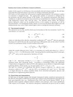
2.3 Fully wet annular fins
Figure 2a is drawn for a schematic representation of an optimum annular fin under
condensation of saturated vapor on its surfaces. The energy equation for one-dimensional
temperature distribution in fully wet annular fins can be written under steady state condition as


() ()( )( )
iiamafg
ddTh
y
rx rx TT h hh
dx dx k

ωω
⎡⎤
⎡
⎤
+=+−+−
⎢⎥
⎣
⎦
⎣⎦
(42)
Eq. (42) is made in dimensionless form by using Eqs. (2) and (3) as



y
x
2r
i
2y
b
l
y
x
O
O
2y
b

l
B

l
0
Wet surface
l
0
Wet surface
Dry surface
Dry surface
A


Fig. 2. Typical configuration of wet fins: A. Annular fin; and B. Spine