Heat Transfer Mathematical Modelling Numerical Methods and Information Technology Part 2 pot

Optimum Fin Profile under Dry and Wet Surface Conditions

29
optimum fins under the volume constraint is less than the surrounding temperature. A
significant change in optimum design variables has been noticed with the design constants
such as fin volume and surface conditions. In order to reduce the complexcity of the
optimum profile fins under different surface conditions, the constraint fin length can be
selected suitably with the constraint fin volume.

0.00 0.01 0.02 0.03 0.04 0.05
0.1
0.2
0.3
0.4
0.5
0.6
0.7
0.8
0.9
1.0
A
U=0.0001
L=0.05
γ
=100%
γ
=70%


θ
X

Fully dry surface
Fully wet surface
0.00 0.01 0.02 0.03 0.04 0.05
0.000
0.001
0.002
0.003
0.004
0.005
B
U=0.0001
L=0.05

Y
X
Fully wet (γ = 100%)
Fully wet (γ = 70%)
Fully dry

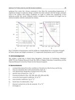
Fig. 9. Variation of temperature and fin profile in a longitudinal fin as a function of length
for both volume and length constraints: A. Temperature distribution; and B. Fin profile
5. Acknowledgement
The authors would like to thank King Mongkut’s University of Technology Thonburi
(KMUTT), the Thailand Research Fund, the Office of Higher Education Commission and the
National Research University Project for the financial support.
6. Nomenclatures
a
constant determined from the conditions of humid air at the fin base and fin tip
b
slop of a saturation line in the psychometric chart, K

– 1

C
non-dimensional integration constant used in Eq. (84)
C
p

specific heat of humid air,
-1 -1
J k
g
K
F
functional defined in Eqs. (10), (28), (46), (62), (80) and (96)
h
convective heat transfer coefficient,
21
W m
-
K
−

h
m

mass transfer coefficient,
21
kg m S

h
fg

latent heat of condensation,
1
J kg
-

k
thermal conductivity of the fin material,
11
W m
-
K
−

l
fin length, m
Heat Transfer - Mathematical Modelling, Numerical Methods and Information Technology

30
l
0

wet length in partially wet fins, m
L
dimensionless fin length,
hl k
L
0

dimensionless wet length in partially wet fins,
0
hl k
Le
Lewis number
q
heat transfer rate through a fin, W
Q
dimensionless heat transfer rate
r
i

base radius for annular fins, m
R
i

dimensionless base radius,
i
hr k
T
temperature, K
U
dimensionless fin volume, see Eqs. (9), (27), (45), (61), (79), (91a) and (95)
V
fin volume (volume per unit width for longitudinal fins), m
3

x, y
coordinates, see Figs. 1 and 2, m

X, Y
dimensionless coordinates,
hx kand hy k , respectively
y
0

semi-thickness of a fin at which dry and wet parts separated, m
Y
0

dimensionless thickness,
0
hy k
Z
1
, Z
2
dimensionless parameters defined in Eqs. (104a) and (104b), respectively
Greek Letters
α

parameter defined in Eqs. (20), (40), (57) and (74a)
λ

Lagrange multiplier
ω

specific humidity of air, kg w. v. / kg. d. a.
ξ

Latent heat parameter
φ
dimensionless temperature,
p
θ
θ
+

0
φ
dimensionless temperature at the fin base,
1
p
θ
+

θ

dimensionless fin temperature,
(
)
(
)
aab
TTTT−−
p
θ

dimensionless temperature parameter, see Eq. (5)
γ

Relative humidity
Subscripts
a ambient
b base
d dewpoint
opt optimum
t tip
7. References
Chilton, T.H. & Colburn, A.P. (1934). Mass transfer (absorption) coefficients–prediction from
data on heat transfer and fluid friction. Ind. Eng. Chem., Vol. 26, 1183.
Duffin, R. J. (1959). A variational problem relating to cooling fins with heat generation. Q.
Appl. Math., Vol. 10, 19-29.
Guceri, S. & Maday, C. J. (1975). A least weight circular cooling fin. ASME J. Eng. Ind., Vol.
97, 1190-1193.
Hanin, L. & Campo, A. (2003). A new minimum volume straight cooling fin taking into
account the length of arc. Int. J. Heat Mass Transfer, Vol. 46, 5145-5152.
Optimum Fin Profile under Dry and Wet Surface Conditions

31
Hong, K. T. & Webb, R. L. (1996). Calculation of fin efficiency for wet and dry fins. HVAC&R
Research, Vol. 2, 27-40.
Kundu, B. & Das, P.K. (1998). Profiles for optimum thin fins of different geometry - A
unified approach. J. Institution Engineers (India): Mechanical Engineering Division,
Vol. 78, No. 4, 215-218.
Kundu, B. (2002). Analytical study of the effect of dehumidification of air on the
performance and optimization of straight tapered fins. Int. Comm. Heat Mass
Transfer, Vol. 29, 269-278.
Kundu, B. & Das, P.K. (2004). Performance and optimization analysis of straight taper fins
with simultaneous heat and mass transfer. ASME J. Heat Transfer, Vol. 126, 862-868.

Kundu, B. & Das, P. K. (2005). Optimum profile of thin fins with volumetric heat generation:
a unified approach. J. Heat Transfer, Vol. 127, 945-948.
Kundu, B. (2007a). Performance and optimization analysis of SRC profile fins subject to
simultaneous heat and mass transfer. Int. J. Heat Mass Transfer, Vol. 50, 1645-1655.
Kundu, B. (2007b). Performance and optimum design analysis of longitudinal and pin fins
with simultaneous heat and mass transfer: Unified and comparative investigations.
Applied Thermal Engg., Vol. 27, Nos. 5-6, 976-987.
Kundu, B. (2008). Optimization of fins under wet conditions using variational principle. J.
Thermophysics Heat Transfer, Vol. 22, No. 4, 604-616.
Kundu, B., Barman, D. & Debnath, S. (2008). An analytical approach for predicting fin
performance of triangular fins subject to simultaneous heat and mass transfer, Int. J.
Refrigeration, Vol. 31, No. 6, 1113-1120.
Kundu, B. (2009a). Analysis of thermal performance and optimization of concentric circular
fins under dehumidifying conditions, Int. J. Heat Mass Transfer, Vol. 52, 2646-2659.
Kundu, B. (2009b). Approximate analytic solution for performances of wet fins with a
polynomial relationship between humidity ratio and temperature, Int. J. Thermal
Sciences, Vol. 48, No. 11, 2108-2118.
Kundu, B. & Miyara, A. (2009). An analytical method for determination of the performance
of a fin assembly under dehumidifying conditions: A comparative study, Int. J.
Refrigeration, Vol. 32, No. 2, 369-380.
Kundu, B. (2010). A new methodology for determination of an optimum fin shape under
dehumidifying conditions. Int. J. Refrigeration, Vol. 33, No. 6, 1105-1117.
Kundu, B. & Barman, D. (2010). Analytical study on design analysis of annular fins under
dehumidifying conditions with a polynomial relationship between humidity ratio
and saturation temperature, Int. J. Heat Fluid Flow, Vol. 31, No. 4, 722-733.
Liu, C. Y. (1961). A variational problem relating to cooling fins with heat generation. Q.
Appl. Math., Vol. 19, 245-251.
Liu, C. Y. (1962). A variational problem with application to cooling fins. J. Soc. Indust. Appl.
Math., Vol. 10, 19-29.
Maday, C. J. (1974). The minimum weight one-dimensional straight fin. ASME J. Eng. Ind.,

Vol. 96, 161-165.
McQuiston, F. C. (1975). Fin efficiency with combined heat and mass transfer. ASHRAE
Transaction, Vol. 71, 350-355.
Mokheimer, E. M. A. (2002). Performance of annular fins with different profiles subject to
variable heat transfer coefficient.
Int. J. Heat Mass Transfer, Vol. 45, 3631-3642.
Heat Transfer - Mathematical Modelling, Numerical Methods and Information Technology

32
Pirompugd, W., Wang, C. C. & Wongwises, S. (2007a). Heat and mass transfer
characteristics of finned tube heat exchangers with dehumidification. J.
Thermophysics Heat transfer, Vol. 21, No. 2, 361-371.
Pirompugd, W., Wang, C. C. & Wongwises, S. (2007b). A fully wet and fully dry tiny
circular fin method for heat and mass transfer characteristics for plain fin-and-tube
heat exchangers under dehumidifying conditions. J. Heat Transfer, Vol. 129, No. 9,
1256-1267.
Pirompugd, W., Wang, C. C. & Wongwises, S. (2008). Finite circular fin method for wavy
fin-and-tube heat exchangers under fully and partially wet surface conditions. Int.
J. Heat Mass Transfer, Vol. 51, 4002-4017.
Pirompugd, W., Wang, C. C. & Wongwises, S. (2009). A review on reduction method for
heat and mass transfer characteristics of fin-and-tube heat exchangers under
dehumidifying conditions. Int. J. Heat Mass Transfer, Vol. 52, 2370-2378.
Razelos, P. & Imre, K. (1983). Minimum mass convective fins with variable heat transfer
coefficient. J. Franklin Institute, Vol. 315, 269-282.
Schmidt, E. (1926). Warmeubertragung durch Rippen. Z. Deustsh Ing., Vol. 70, 885-951.
Solov”ev, B.A. (1968). An optimum radiator-fin profile. Inzhenerno Fizicheskii Jhurnal, Vol. 14,
No. 3, 488-492.
Threlkeld, J. L. (1970). Thermal environment engineering. Prentice-Hall, New York.
Wilkins, J. E. Jr. (1961). Minimum mass thin fins with specified minimum thickness. J. Soc.
Ind. Appl. Math., Vol. 9, 194-206.

Wu, G. & Bong, T. Y. (1994). Overall efficiency of a straight fin with combined heat and mass
transfer. ASRAE Transation, Vol. 100, No. 1, 365-374.
Zubair, S. M.; Al-Garni, A. Z. & Nizami, J. S. (1996). The optimum dimensions of circular
fins with variable profile and temperature-dependent thermal conductivity. Vol. 39,
No. 16, 3431-3439.

0
Thermal Therapy: Stabilization and Identification
Aziz Belmiloudi
Institut National des Sciences Appliqu´ees de Rennes (INSA)
Institut de Recherche MAth´ematique de Rennes ( IRMAR), Rennes
France
1. Introduction
1.1 Terminology and m ethods
The physicists, biologists or chemists control, in general, their experimental devices by using
a certain number of functions or parameters of control which enable them to optimize and
to stabilize the system. The work of the engineers consists in determining theses functions
in an optimal and stable way in accordance with the desired performance. We can note that
the three main steps in the area of research in control of dynamical systems are inextricably
linked, as shown below:
To predict the response of dynamic systems from given parameters, data and source terms
requires a mathematical model of the behaviour of the process under investigation and
a physical theory linking the state variables of the model to data and parameters. This
prediction of the observation (i.e. modeling) constitutes the so-called direct problem (primal
problem, prediction problem or also forward problem) and it is usually defined by one or more
coupled integral, ordinary or partial differential systems and sufficient boundary and initial
conditions for each of the main fields (such as temperature, concentration, velocity, pressure,
wave, etc.). Initial and boundary conditions are essential for the design and characterization
of any physical systems. For example, in a transient conduction heat transfer problem, in
order to define a ”direct heat conduction problem”, in addition to the model which include

thermal conductivity, specific heat, density, initial temperature and other data, temperature,
flux or radiating boundary conditions are applied to each part of the boundary of the studied
domain.
Direct problems are well-posed problem in the sense of Hadamard. Hadamard claims that
a mathematical model for a physical problem has to be well-posed or properly problem in
the sense that it is characterized by the existence of a unique solution that is stable (i.e. the
solution depends continuously on the given data) to perturbations in the given data (material
properties, boundary and initial conditions, etc.) under certain regularity conditions on data
and additional properties. The requirement of stability is the most important one, because if
this property is not valid, then the problem becomes very sensitive to small fluctuations and
noises (chaotic situation) and consequently it is impossible to solve the problem.
2
2 Heat Transf er
If any of the conditions necessary to define a direct problem are unknown or rather badly
known, an inverse problem (control problem or protection problem) results, typically when
modeling physical situations where the model parameters (intervening either in the boundary
conditions, or initial conditions or equations model itself) or material properties are unknown
or partially known. Certain parameters or data can influence considerably the material
behavior or modify phenomena in biological or medical matter; then their knowledge (e.g.
parameter identification) is an invaluable help for the physicists, biologists or chemists who,
in general, use a mathematical model for their problem, but with a great uncertainty on its
parameters. The resolution of the inverse problems thus provides them essential informations
which are necessary to the comprehension of the various processes which can intervene in
these models. This resolution need some regularity and additional conditions, and partial
informations of some unknown parameters and fields (observations) given, for example, by
experiment measurements.
In all cases the inverse problem is ill-posed or improperly posed (as opposed to the well-posed
or properly problem in the sense of Hadamard) in the sense that conditions of existence
and uniqueness of the solution are not necessarily satisfied and that the solution may be
unstable to perturbation in input data (see (Hadamard, 1923)). The inverse problem is

used to determine the unknown parameters or control certain functions for problems where
uncertainties (disturbances, noises, fluctuations, etc.) are neglected. Moreover the inverse
problems are not always tolerant to changes in the control system or the environment. But it is
well known that many uncertainties occur in the most realistic studies of physical, biological
or chemical problems. The presence of these uncertainties may induce complex behaviors,
e.g., oscillations, instability, bad performances, etc. Problems with uncertainties are the most
challenging and difficult in control theory but their analysis are necessary and important for
applications.
If uncertainties, stability and performance validation occur, a robust control problem results.
The fundament of robust control theory, which is a generalization of the optimal control
theory, is to take into account these uncertain behaviours and to analyze how the control
system can deal with this problem. The uncertainty can be of two types: first, the errors (or
imperfections) coming from the model (difference between the reality and the mathematical
model, in particular if some parameters are badly known) and, second, the unmeasured noises
and fluctuations that act on the physical, biological or chemical systems (e.g. in medical
laser-induced thermotherapy (ILT), a small fluctuation of laser power can affect considerably
the resulting temperature distribution and thus the cancer treatment). These uncertainty terms
can have additive and/or multiplicative components and they often lead to great instability.
The goal of robust control theory is to control these instabilities, either by acting on some
parameters to maintain the system in a desired state (target), or by calculating the limit of
these parameters before the system becomes unstable (”predict to act”). In other words,
the robust control allows engineers to analyze instabilities and their consequences and helps
them to determine the most acceptable conditions for which a system remains stable. The
goal is then to define the maximum of noises and fluctuations that can be accepted if we
want to keep the system stable. Therefore, we can predict that if the disturbances exceed this
threshold, the system becomes unstable. It also allows us, in a system where we can control
the perturbations, to provide the threshold at which the system becomes unstable.
Our robust control approach consists in setting the problem in the worst-case disturbances
which leads to the game theory in which the controls and the disturbances (which destabilize
the dynamical behavior of the system) play antagonistic roles. For more details on this new

34
Heat Transfer - Mathematical Modelling, Numerical Methods and Information Technology
Thermal Therapy: Stabilization and Identification 3
approach and its application to different models describing realistic physical and biological
process, see the book (Belmiloudi, 2008).
We shall now present the process of our control robust approach.
1.2 General process of the r obust c ontrol technique
In contrast with the inverse (or optimal control) problems
1
, the relation between the problems
of identification, regulation and optimization, lies in the fact that it acts, in these cases, to
find a saddle point of a functional calculus depending on the control, the disturbance and
the solution of the direct perturbation problem. Indeed, the problems of control can be
formulated as the robust regulation of the deviation of the systems from the desired target; the
considered control and disturbance variables, in this case, can be in the parameters or in the
functions to be identified. This optimization problem (a minimax problem), depending on the
solution of the direct problem, with respect to control and disturbance variables (intervening
either in the initial conditions, or boundary conditions or equation itself), is the base of the
robust control theory of partial differential equations (see (Belmiloudi, 2008)).
The essential data used in our robust control problem are the following.
• A known operator F which represents the dynamical system to be controlled i.e. F is the
model of the studied boundary-value problem such that
F(x, t, f,g,U)=0, (1)
where
(x, t) are the space-time variables, ( f , g) ∈Xrepresents the input of the system
(initial conditions, boundary conditions, source terms, parameters and others) and U
∈Z
represents the state or the output of the system (temperature, concentration, velocity,
magnetic field, pressure, etc.), where
X and Z are two spaces of input data and output

solutions, respectively, which are assumed to be, for example, Hilbert and Banach spaces,
respectively. We assume that the direct problem (1) is well-posed (or correctly-set) in
Hadamard sense.
• A “control” variable ϕ in a set U
ad
⊂U
1
(known as set of “admissible controls”) and a
“disturbance” variable ψ in a set V
ad
⊂U
2
(known as set of “admissible disturbances”),
where
U
1
and U
2
are two spaces of controls and disturbances, respectively, which are
assumed to be, for example, Hilbert spaces.
• For a chosen control-disturbance (ϕ, ψ),theperturbation problem,whichmodels
fluctuations
(ϕ,ψ,u) to the desired target ( f , g,U) (we assume that ( f + B
1
ϕ, g + B
2
ψ, U +
u) is also solution of (1)) and which is given by
˜
F(x, t, ϕ, ψ, u)=F(x, t, f + B

1
ϕ, g + B
2
ψ, U + u) −F(x, t, f,g,U)=0, (2)
where the operator
˜
F, which depends on U, is the perturbation of the model F of the
studied system and
B
i
,fori = 1,2, are bounded linear operators from U
i
into Z.Inthe
sequel we denote by u
= M(x, t, ϕ, ψ) the solution of the direct problem (2).
• An “observation” u
obs
which is supposed to be known exactly (for example the desired
tolerance for the perturbation or the offset given by measurements).
1
Inverse problem corresponds to minimize or maximize a calculus function depending on the control
and the solution of the direct problem.
35
Thermal Therapy: Stabilization and Identification
4 Heat Transf er
• A “cost” functional (or “objective” functional) J(ϕ, ψ) which is defined from a real-valued
and positive function
G(X,Y) by (so-called the reduced form)
J
(ϕ,ψ)=G((ϕ, ψ), M(., ϕ, ψ)).

The goal is to find a saddle point of J, i.e.,asolution
(ϕ
∗
,ψ
∗
) ∈ U
ad
×V
ad
of
J
(ϕ,ψ
∗
) ≤ J(ϕ
∗
,ψ
∗
) ≤ J(ϕ
∗
,ψ) ∀(ϕ, ψ) ∈ U
ad
×V
ad
,
i.e. find
(ϕ
∗
,ψ
∗
,u

∗
) ∈ U
ad
× V
ad
×Zsuch that the cost functional J is minimized with
respect to ϕ and maximized with respect to ψ subject to the problem (2) (i.e. u
∗
(x, t)=
M(
x, t, ϕ
∗
,ψ
∗
)).
We lay stress upon the fact that there is no general method to analyse the problems of robust
control (it is necessary to adapt it in each situation). On the other hand, we can define a process
to be followed for each situation.
(i) solve the direct problem (existence of solutions, uniqueness, stability according to the data,
regularity, etc.)
(ii) define the function or the parameter to be identified and the type of disturbance to be
controlled
(iii) introduce and solve the perturbed problem which plays the role of the direct
problem (existence of solutions, uniqueness, stability according to the data, regularity,
differentiability of the operator solution, etc.)
(iv) define the cost (or objective) functional, which depends on control and disturbance
functions
(v) obtain the existence of an optimal solution (as a saddle point of the cost functional) and
analyse the necessary conditions of optimality
(vi) characterize the optimal solutions by introducing an adjoint (dual or co-state) model (the

characterization include the direct problem coupled with the adjoint problem, linked by
inequalities)
(vii) define an algorithm allowing to solve numerically the robust control problem.
Remark 1
1. In nonlinear systems the analysis of robust control problems is more complicated than in the case of
inverse problems, because we are interested in the robust regulation of the deviation of the systems
from the desired target state variables (while the desired power level and adju stment costs are taken
into consideration) by analyzing the full nonlinear systems which model large perturbations to the
desired target. Consequently the perturbations of the initial models, which show additional operators
(and then difficulties), generate new direct problem and then new adjoint problem which, often, seem
of a new type.
2. If there are no noises (i.e.,
B
2
vanishes), the problem becomes an inverse problem or model
calibration, i.e., find ϕ in U
ad
such that the cost functional J
0
(ϕ) (in reduced form i.e. in place
of the form
G
0
(ϕ,U = M(., ϕ))) is minimized subject to the well-posed problem
F(x, t, f
0
+ B
1
ϕ, g, U)=0, (3)
36

Heat Transfer - Mathematical Modelling, Numerical Methods and Information Technology
Thermal Therapy: Stabilization and Identification 5
where data ( f
0
, g) are known (we have supposed that f is decomposed into a known function f
0
and
the control ϕ)andM
(., ϕ)=U is the solution of (3), corresponding to ϕ. Precisely, the problem is
:find
(ϕ
∗
,U
∗
) ∈ U
ad
×Zsolution of
J
0
(ϕ
∗
)= inf
ϕ∈U
ad
J
0
(ϕ),
and U
∗
= M(., ϕ

∗
).
2. Statement of the problem
2.1 Prob lem definition
Motivated by topics and issues critical to human health and safety of treatment, the problem
studied in this chapter derives from the modeling and stabilizing control of the transport of
thermal energy in biological systems with porous structures.
The evaluation of thermal conductivities in living tissues is a very complex process which
uses different phenomenological mechanisms including conduction, convection, radiation,
metabolism, evaporation and others. Moreover blood flow and extracellular water affect
considerably the heat transfer in the tissues and then the tissue thermal properties. The
bioheat transfer process in tissues is also dependent on the behavior of blood perfusion along
the vascular system. An analysis of thermal process and corresponding tissue damage taking
into account theses parameters will be very beneficial for thermal destruction of the tumor in
medical practices, for example for laser surgery and thermotherapy for treatment planning
and optimal control of the treatment outcome, often used in treatment of cancer. The first
model, taking account on the blood perfusion, was introduced by Pennes see (Pennes, 1948)
(see also (Wissler, 1998) where the paper of Pennes is revisited). The model is based on
the classical thermal diffusion system, by incorporating the effects of metabolism and blood
perfusion. The Pennes model has been adapted per many biologists for the analysis of
various heat transfer phenomena in a living body. Others, after evaluations of the Pennes
model in specifical situations, have concluded that many of the hypotheses (foundational
to the model) are not valid. Then these latter ones modified and generalized the model to
adequate systems, see e.g. (Chen & Holmes, 1980a;b);(Chato, 1980); (Valvano et al., 1984);
(Weinbaum & Jiji, 1985); (Arkin et al., 1986); (Hirst, 1989) (see also e.g. (Charney, 1992) for a
review on mathematical modeling of the influence of blood perfusion). Recently, some studies
have shown the important role of porous media in modeling flow and heat transfer in living
body, and the pertinence of models including this parameter have been analyzed, see e.g.
(Shih et al., 2002); (Khaled & Vafai, 2003); (Belmiloudi, 2010) and the references therein.
The goal of our contribution is to study time-dependent identification, regulation and

stabilization problems related to the effects of thermal and physical properties on the transient
temperature of biological tissues with porous structures. To treat the system of motion in
living body, we have written the transient bioheat transfer type model in a generalized form by
taking into account the nature of the porous medium. In paragraph 3.1, we have constructed
a model for a specific problem which has allowed us to propose this generalized model as
follows
c
(φ, x)
∂U
∂t
= div (κ(φ, U, x)∇U) −e(φ, x)P(x, t)(U −U
a
)
−
d(φ, x)K
v
(U)+r(φ, x)g(x, t)+ f (x, t) in Q,
subjected to the boundary condition
(4)
37
Thermal Therapy: Stabilization and Identification
6 Heat Transf er
(κ(φ,U, x)∇U).n = −q(x, t )(U −U
b
)
−λ(x)( L(U) − L(U
b
)) + h(x, t) in Σ,
and the initial condition
U

(x,0)=U
0
(x) in Ω,
under the pointwise constraints
a
1
≤ P ≤ a
2
a.e. in Q,
b
1
≤ φ ≤ b
2
a.e. in Ω,
(5)
where the state function U is the temperature distribution, the function K
v
is the transport
operator in

ϑ direction i.e. K
v
(U)=(

ϑ.∇)U, the function L is the radiative operator i.e.
L
(U)=| U |
3
U.ThebodyΩ is an open bounded domain in IR
m

, m ≤ 3 with a smooth
boundary Γ
= ∂Ω which is sufficiently regular, and Ω is totally on one side of Γ, the cylindre Q
is Q = Ω ×(0, T) with T > 0 a fixed constant (a given final time), Σ = ∂Ω ×(0, T), n is the unit
outward normal to Γ and a
i
, b
i
,fori = 1,2, are given positive constants. The quantity P is the
blood perfusion rate and φ
∈ L
∞
(Ω) describes the porosity that is defined as the ratio of blood
volume to the total volume (i.e. the sum of the tissue domain and the blood domain). The
volumetric heat capacity type function c
(φ,.) and the thermal conductivity type function of
the tissue κ
(φ,U,.) are assumed to be variable and satisfy ν ≥ κ(φ, U,.)=σ
2
(φ,U,.) ≥ μ > 0,
M
1
≥ c( φ,.)=x
2
(φ,.) ≥ M
0
> 0(whereν, μ, M
0
, M
1

are positive constants). The second
term on the right of the state equation (4) describes the heat transport between the tissue
and microcirculatory blood perfusion, the third term K
v
is corresponding to the directional
convective mechanism of heat transfer due to blood flow, the last terms are corresponding
to the sum of the body heating function which describes the physical properties of material
(depending on the thermal absorptivity, on the current density, on the electric field intensity,
that can be calculated from the Maxwell equations, and others) and the source terms that
describe a distributed energy source which can be generated through a variety of sources,
such as focused ultrasound, radio-frequency, microwave, resistive heating, laser beams and
others (depending on the difference between the energy generated by the metabolic processes
and the heat exchanged between, for example, the electrode and the tissue). The first term in
the right of the boundary condition in (4) describes the convective component and the second
term is the radiative component. The term h is the heat flux due to evaporation. The function
U
a
is the arterial blood temperature, the function U
b
is the bolus temperature and they are
assumed to be in L
∞
(Q) and in L
∞
(Σ), respectively.
The function u
0
is the initial value and is assumed to be variable and λ = σ
B


e
is assumed
to be in L
∞
(Γ) where σ
B
(Wm
−2
K
−4
) is Stefan-Boltzmann’s constant and 
e
is the effective
emissivity. The vector function

ϑ is the flow velocity which is assumed to be sufficiently
regular.
Remark 2
1. Emissivity of a material is defined as the ratio of energy radiated by a particular material to
energy radiated by a black body at the same temperature (the tissue is not a perfect black body).
It is a dimensionless quantity (i.e. a quantity without a physical unit). The emissivity of human
skin is in the range 0.98
−0.99.
38
Heat Transfer - Mathematical Modelling, Numerical Methods and Information Technology
Thermal Therapy: Stabilization and Identification 7
2. We consider only the boundary effect of the process of radiation, since radiative heat transfer
processes within the system are neglected.
3. In the physical case there is not absolute values under the boundary conditions (since the
temperature is non negative). For real physical and biological data, we can prove by using

the maximum principle that the temperature is positive and then we can remove the absolute
values.
4. For all

ϑ sufficiently regular (such e.g. the condition (17)), the linear operator satisfies the
following estimate:
there exists a constant γ
v
≥ 0 (depending on the norm of

ϑ)suchthat
 K(

ϑ, v) 
L
2
(Ω )
≤ γ
v
 v 
H
1
(Ω )
,∀v ∈ H
1
(Ω).(6)
5. The nonlinear scalar function L : IR
−→ IR i s a C
1
(IR ) function and its derivative is given by

L

(v)=4 | v |
3
.(7)
2.2 Basis for thermal therapy
Cells, vasculature (which supply the tissue with nutrients and oxygen through the flow
of blood) and extracellular matrix (which provides structural support to cells) are the
main constituents of tissue. Most living cells and tissues can tolerate modest temperature
elevations for limited time periods depending on the metabolic status of the individual cell
(so-called thermotolerance). Contrariwise, when tissues are exposed to very high temperature
conditions, this leads to cellular damage which can be irreversible.
Therapy by elevation of temperature is a thermal treatment in which pathological tissue
is exposed to high temperatures to damage and destroy or kill malignant cells (directly or
indirectly by the destruction of microvasculature) or to make malignant cells more sensitive
to the effects of another therapeutic option, such as radiation therapy, chemotherapy or
photodynamic therapy. Many scientists claim that this is due largely to the difference in
blood circulation between tumor and normal tissues. Moreover, local tissue properties, in
particular perfusion, have a significant impact on the size of treatment zone, for example,
highly perfused tissue and large vessels act as a heat sink (this phenomenon makes normal
tissue relatively more resilient to treatment than tumor tissue, since perfusion rates in tumors
are generally less than those in normal tissues). Consequently, the knowledge of the thermal
properties and blood perfusion of biological tissues is fundamental for accurately modeling
the heat transfer process during thermal therapy. The most commonly used technique for
heating of tumors is the interstitial thermal therapy, in which heating elements are implanted
directly into the treated zone, because energy can be localized to the target region while
surrounding healthy tissue is preserved. Different energy sources are employed to deliver
local thermal energy including laser, microwaves, radiofrequency and ultrasound.
The traditional hyperthermia is defined as a temperature greater than 37.5
−38.3

o
C, in general
in the interval of about 41
− 47
o
C. This thermal therapy is only useful for certain kinds of
cancer and is most effective when it is combined with the other conventional therapeutic
modalities. Though temperatures are not very high and then cell death is not instantaneous,
prolonged exposure leads to the thermal denaturation of non-stabilized proteins such as
enzymes and to their destruction, which ultimately leads to cell death. There are various types
of hyperthermia as alternative cancer therapy. These include: the regional (heats a larger part
of the body, such as an entire affected organ) and local (heats a small area, such as the tumor
39
Thermal Therapy: Stabilization and Identification
8 Heat Transf er
itself) hyperthermia, where temperatures reach between 42 and 44
o
C and the whole body
hyperthermia, where the entire body except for the head is overheated to a temperature of
about 39 to 41
o
C. Heat sensitivity of the tissue is lost at higher temperatures (above 44
o
C)
resulting in tumor and normal tissues destruction at the same rate. Consequently, in order
to minimize damage to surrounding tissues and other adverse effects, we must keep local
temperatures under 44
o
C, but requires more treatment-time (between 1 and 3 hours). At these
low temperatures damage can be reversible. Indeed damaged proteins can be repaired or

degraded and replaced with new ones.
For a rapid destruction of tissue, it is necessary to make a temperature rise of at least
exceed 50
o
C. During thermotherapy, which employs higher temperatures over shorter times
(seconds to minutes), than those used in hyperthermia treatment, several processes, as tissue
vaporization, carbonization and molecular dissociation, occur which lead to the destruction
or death of the tissue. At temperatures above 60
o
C, proteins and other biological molecules of
the tissue become severely denatured (irreversibly altered) and coagulate leading to cell and
tissue death. Temperatures above 100
o
C will cause vaporization from evaporation of water
in the tissue and in the intracellular compartments and lead to rupture or explosion of cells
or tissue components, and above 300
o
C tissue carbonization occurs. At these temperatures,
an elevated temperature front migrates through the tissue and structural proteins, such as
fibrillar collagen and elastin, begin to damage irreversibly causing visible whitening of the
tissue and then coagulation necrosis to the targeted tissue. Indeed, structural proteins are
more thermally stable than the intracellular proteins and enzymes (involved in reversible heat
damage), and consequently tissue coagulation signifies destruction of the lesion.
The actual level of thermal damage in cells and tissue is a function of both temperature
and heating time. Using the temperature history, the accumulation of thermal damage,
associated with injury of tissue, can be calculated by an approach (based on the well-known
Arrhenius model see e.g. (Henriques, 1947)) characterizing tissue damage, including cell kill,
microvascular stasis and protein coagulation. For this, we can use the Arrhenius damage
integral formulation, which assumes that some thermal damage processes follow first-order
irreversible rate reaction kinetics (from thermal chemical rate equations, see e.g. (Atkins,

1982)), for more details see e.g. (Tropea & Lee, 1992) and (Skinner et al., 1998):
D(x, τ
ex p
)=ln(
C(0)
C(τ
ex p
)
)=
A

τ
exp
0
ex p(
−
E
RU (x, t)
)
dt,(8)
where D is the nondimensional degree of tissue injury, U is the temperature of exposure (K ),
τ
ex p
is the duration of the exposure, C(0) is the concentration of living cells before irradiation
exposure and C
(τ
ex p
) is the concentration of living cells at the end of the exposure time. The
parameter A is the molecular collision frequency (s
−1

) i.e. damage rate, the parameter E is the
denaturation activation energy (J.mol
−1
)andR is the universal gaz constant equal to 8.314
J.mol
−1
K
−1
. The two kinetic parameters A and E are dependent on the type of tissue and
must be determined by experiments a priori. The cumulative damage can be interpreted as
the fraction of hypothetical indicator molecules that are denatured and can play an important
role in the optimization of the treatment.
Other cell damage models are developed, in recent years, see for example the two-state model
of Oden et al. in (Feng et al., 2008) (which is based on statistical thermodynamic principles) as
follows:
D(x, τ
ex p
)=

τ
exp
0
1
1 + ex p(
−E
o
(t,U(x,t))
RU (x,t)
)
dt,(9)

40
Heat Transfer - Mathematical Modelling, Numerical Methods and Information Technology
Thermal Therapy: Stabilization and Identification 9
with the activation energy function E
0
(t,U)=(
ζ
U
+ at + b),whereζ, a and b are known
constants determined by in vitro cellular experiments.
In conclusion the cell damage model can be expressed by the following general form
D(x, τ
ex p
)=ln(
C(0)
C(τ
ex p
)
)=

τ
exp
0
H(t, U(x, t))dt, (10)
where
H is differentiable on the variable U.
2.3 Outline
We give now the outline of the rest of the chapter. First, the modeling of thermal transport
by perfusion within the framework of the theory of porous media is presented and the
governing equations are established. The thermal processes within the tissues are predicted

by using some generalized uncertain evolutive nonlinear bioheat transfer type models
with nonlinear Robin boundary conditions (radiative type), by taking into account porous
structures and directional blood flow. Afterwards the existence, the uniqueness and the
regularity of the solution of the state equation are presented as well as stability and maximum
principle under extra assumptions. Second, we introduce the initial perturbation problem
and give the existence and uniqueness of the perturbation solution and obtain a stability
result. Third, the real-time identification and robust stabilization problems are formulated,
in different situations, in order to reconstitute simultaneously the blood perfusion rate, the
porosity parameter, the heat transfer parameter, the distributed energy source terms and
the heat flux due to the evaporation, which affect the effects of thermal physical properties
on the transient temperature of biological tissues, and to control and stabilize the desired
online temperature and thermal damage provided by MRI (Magnetic Resonance Imaging)
measurements. Because, it is now well-known that a controlled and stabilized temperature
field does not necessarily imply a controlled and stabilized tissue damage. This work includes
results concerning the existence of the optimal solutions, the sensitivity problems, adjoint
problems, necessary optimality conditions (necessary to develop numerical optimization
methods) and optimization problems. Next, we analyse the case when data are measured
in only some points in space-time domain, and the case where the body Ω is constituted by
different tissue types which occupy finitely many disjointed subdomains. As in previous, we
give the existence of an optimal solution and we derive necessary optimality conditions. Some
numerical strategies, based on adjoint control optimization (combining the obtained optimal
necessary conditions and gradient-iterative algorithms), in order to perform the robust
control, are also discussed. Finally, control and stabilization problems for a coupled thermal,
radiation transport and coagulation processes modeling the laser-induced thermotherapy in
biological tissues, during cancer treatment, are analyzed.
In the sequel, we will always denoted by C some positive constant which can be different at
each occurrence.
3. Mathematical modelling and motivation
3.1 Model d evelopment
3.1.1 Heat transfer equation

The blood-perfused tumor tissue volume, including blood flow in microvascular bed with
the blood flow direction, contains many vessels and can be regarded as a porous medium
consisting of a tumor tissue (a solid domain) fully filled with blood (a liquid domain), see
41
Thermal Therapy: Stabilization and Identification
10 Heat Transf er
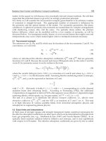
Figure 1. Consequently the temperature distribution in biological tissue can be modelized by
analyzing a conjugate heat transfer problem with the porous medium theory. For the tumor
tissue domain, we use the Pennes bioheat transfer equation by taking account on the blood
perfusion in the energy balance for the blood phase. For the blood flow domain, we use the
energy transport equation. The system of equations of the model is then
c
s
(x)ρ
s
(x)
∂U
s
∂t
= div (κ
s
(U
s
, x)∇U
s
) −c
l
(x)w
l
(x, t)(U

s
−U
a
)+Q
s
(x, t)+Q
J
(x, t),
c
l
(x)ρ
l
(x)(
∂U
l
∂t
+(

ϑ.∇)U
l
)=di v (κ
l
(U
l
, x)∇U
l
)+Q
J
(x, t),
(11)

where c
l
, c
s
, ρ
l
, ρ
s
, U
l
, U
s
, κ
l
, κ
s
, Q
s
, Q
J
are the specific heat of blood, the specific heat
of tissue, the density of blood, the density of tissue, the local blood temperature, local
tissue temperature, blood effective thermal conductivity tensor, tissue effective thermal
conductivity tensor, metabolic volumetric heat generation and energy source term (which is
also called the specific absorption rate, SAR (Wm
−3
)), respectively, and U
a
is the temperature
in arterial blood. The term di v

(κ
l
(U
l
)∇U
l
) is corresponding to the enhancement of thermal
conductivity in tissue due to the flow of blood within thermally significant blood vessels and
the term div
(κ
s
(U
s
)∇U
s
) is similar to Pennes model. The transport operator is

ϑ.∇ and is
corresponding to a directional convective term due to the net flux of the equilibrated blood.
Fig. 1. : Relationship between tumor vascular and blood flow direction
The volumetric averaging of the energy conservation principle is achieved by combining and
rearranging the first and the second part of the system (11) with the porous structure (regarded
as a homogeneous medium). Under thermal equilibrium and according to the modelization
of (Chen & Holmes, 1980a) (the model has been formulated after the analyzing of blood vessel
thermal equilibration length) we have then by multiplying the first equation by
(1 − φ) and
the second equation by φ
((1 − φ)c
s
(x)ρ

s
(x)+φc
l
(x)ρ
l
(x))
∂U
∂t
+ div (((1 −φ)κ
s
(U, x)+φκ
l
(U, x))∇U)
+
φc
l
(x)ρ
l
(x)(

ϑ.∇) U +(1 −φ) c
l
(x)w
l
(x, t)(U −U
a
)=(1 −φ)Q
s
(x, t)+Q
J

(x, t).
(12)
Our model incorporates the effect of blood flow in the heat transfer equation in a way that
captures the directionality of the blood flow and incorporates the convection features of the
heat transfer between blood and solid tissue.
42
Heat Transfer - Mathematical Modelling, Numerical Methods and Information Technology
Thermal Therapy: Stabilization and Identification 11
The model (12) is a particular case of the general equation in the system (4), by taking, in the
first relation of (4), the heat capacity type function c
(φ, x) as (1 −φ)c
s
ρ
s
+ φc
l
ρ
l
,thethermal
conductivity capacity type function κ
(φ,U, x) as (1 − φ)κ
s
+ φκ
l
, the function e(φ, x )P(x, t) as
(1 −φ)c
l
w
l
, the function d(φ, x) as φc

l
ρ
l
, the function r(φ, x) as 1 −φ, the function f as Q
J
and
the function g as Q
s
.
To close the model, we must specify boundary conditions.
3.1.2 Boundary conditions
Every body emits electromagnetic radiation proportional to the fourth power of the absolute
temperature of its surface. The total energy, emitted from a black body, E
R
(Wm
−2
)canbe
given by the following Stefan-Boltzmann-Law:
E
R
= σ
B

e
(U
4
−U
4
b
), (13)

where σ
B
= 5.67.10
−8
Wm
−2
K
−4
is the Stefan-Boltzmann constant, U and U
b
(K) are the tissue
surface temperature and surrouding temperature, respectively and 
< 1 (since tissue is not a
perfect black body) is the emissivity coefficient.
Convection problems involve the exchange of heat between the surface of the body (the
conducting) and the surrounding air (convecting). The thermal energy E
C
(Wm
−2
)canbe
given by Newton’s law of cooling:
E
C
= q(U −U
b
), (14)
where, the proportionality function q (Wm
−2
K
−1

) is the coefficient of local heat convection
and U
b
is the bulk temperature of the air (assumed to be similar as relation in (13)).
If we assume that the evaporation occurs mainly at the surface, the energy associated with the
phase change occurring during evaporation (the heat flux due to evaporation) can be given
by the following expression
E
V
= h
fg
m
w
= −h(x, t), (15)
where h
fg
is the latent heat of vaporization and m
w
is the mass flux of evaporating water.
According to the previous relations, the boundary condition can be imposed as follows:
−(κ(φ, U, x)∇U).n = E
R
+ E
C
+ E
V
= q(U −U
b
)+λ(x)( L(U) − L (U
b

)) − h(x, t), (16)
where λ
= σ
B

e
and L(v)=|v |
3
v = v
4
for all positive functions.
We recall now some biological and medical background and motivations to analyse the
identification, calibration and stabilization problem.
3.2 Bac kground and motivation
Mathematical modeling of cancer treatments (chemotherapy, thermotherapy, etc) is an highly
challenging frontier of applied mathematics. Recently, a large amount of studies and research
related to the cancer treatments, in particular by chemotherapy or thermotherapy, have been
the object of numerous developments.
As an alternative to the traditional surgical treatment or to enhance the effect of
conventional chemotherapy, various problems associated with localized thermal
therapy have been intensively studied (see e.g. (Pincombe & Smyth, 1991);
(Hill & Pincombe, 1992); (Tropea & Lee, 1992); (Martin et al., 1992); (Seip & Ebbini,
1995); (Sturesson & Andersson-Engels, 1995); (Deuflhard & Seebass, 1998); (Xu et al.,
43
Thermal Therapy: Stabilization and Identification
12 Heat Transf er
1998); (Liu et al., 2000); (Marchant & Lui, 2001); (Shih et al., 2002); (He & Bischof, 2003);
(Zhou & Liu, 2004); (Zhang et al., 2005) and the references therein). In order to improve
the treatments, several approaches have been proposed recently to control the temperature
during thermal therapy. We can mention e.g. (Bohm et al., 1993); (Hutchinson et al., 1998);

(K¨ohler et al., 2001); (Vanne & Hynynen, 2003); (Kowalski & Jin, 2004); (Malinen et al., 2006);
(Belmiloudi, 2006; 2007) and the references therein. The essential of these contributions has
been the numerical analysis, MRI-based optimization techniques and mathematical analysis.
For the stabilization of the temperature treatment, see e.g. (Belmiloudi, 2008), in which the
author develops nonlinear PDE robust control approach in order to stabilize and control the
desired online temperature for a Pennes’s type model with linear boundary conditions.
An important application of all bioheat transfer models in interdisciplinary research areas,
in joining mathematical, biological and medical fields, is the analysis of the temperature
field which develops in living tissue when a heat is applied to the tissue, especially in
the clinical cancer therapy hyperthermia and in the accidental heating injury, such as
burns (in hyperthermia, tissue is heated to enhance the effect of an accompanying radio or
chemotherapy). Indeed the thermal therapy (performed with laser, focused ultrasound or
microwaves) gives the possibility to destroy the pathological tissues with minimal damage
to the surrounding tissues. Moreover, due to the self-regulating capability of the biological
tissue, the blood perfusion and the porosity parameters depend on the evolution of the
temperature and vary significantly between different patients, and between different therapy
sessions (for the same patient). Consequently, in order to have a very optimal thermal
diagnostics and so the result of the therapy being very beneficial to treatment of the patient, it
is necessary to identify the value of these two parameters.
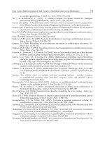
The new feature introduced in this work concerns the estimation of the evolution of the
blood perfusion and the porosity parameters by using nonlinear optimal control methods,
for some generalized evolutive bioheat transfer systems, where the observation is the online
temperature control provided by Magnetic Resonance Imaging (MR I) measurements, see
Figure2 (MRI is a new efficient tool in medicine in order to control surgery and treatments).
(a) Control process (b) Applicator and measurements
Fig. 2. : Laser-induced thermotherapy and identification
44
Heat Transfer - Mathematical Modelling, Numerical Methods and Information Technology
Thermal Therapy: Stabilization and Identification 13
The introduction of the theory of porous media for heat transfer in biological tissues is

very important because the physical properties of material have power law dependence
on temperature (see e.g. (Marchant & Lui, 2001; Pincombe & Smyth, 1991)) and moreover
the porosity is one of the crucial factors determining distribution of temperature during
thermal therapies, for example in medical laser-induced thermotherapy (see e.g. the review
of (Khaled & Vafai, 2003)). Consequently we cannot neglect the influence of the porosity in
the model and then it is necessary to identify, in more of the blood perfusion, the porosity
of the material during thermal therapy in order to maximize the efficiency and safety of
the treatment. Moreover, the introduction of the nonlinear radiative operator including the
cooling mechanism of water evaporation in the model is very important, because the heat
exchange mechanisms at the body-air interface play a very important part on the total tissue
temperature distribution and consequently we cannot also neglect the influence of the surface
evaporation in the model (see e.g. (Sturesson & Andersson-Engels, 1995)). On the other hand
we will consider that the source term f and the heat flux due to evaporation h (in the model
(4)) are not accurately known.
4. Solvability of the state system
Now we give some assumptions, notations, results and an analysis of the state system (4)
which are essential for the following investigations.
4.1 Assumptions and notations
We use the standard notation for Sobolev spaces (see (Adams, 1975)), denoting the norm
of W
m,p
(Ω) (m ∈ IN , p ∈ [ 1, ∞])by
W
m,p
(Ω )
.Inthespecialcasep = 2weuseH
m
(Ω)
instead of W
m,2

(Ω). The duality pairing of a Banach space X with its dual space X

is
given by
< .,. >
X

,X
. For a Hilbert space Y the inner product is denoted by (.,.)
Y
.Forany
pair of real numbers r, s
≥ 0, we introduce the Sobolev space H
r,s
(Q) defined by H
r,s
(Q)=
L
2
(0, T, H
r
(Ω)) ∩ H
s
(0, T, L
2
(Ω)), which is a Hilbert space normed by
( v 
2
L
2

(0,T,H
r
(Ω ))
+ v 
2
H
s
(0,T,L
2
(Ω ))
)
1/2
,
where H
s
(0, T, L
2
(Ω)) denotes the Sobolev space of order s of functions defined on (0, T)
and taking values in L
2
(Ω),anddefinedby,forθ ∈ (0,1), s =(1 − θ)m, m is an integer, (see
e.g. (Lions & Magenes, 1968)) H
s
(0, T, L
2
(Ω)) = [ H
m
(0, T, L
2
(Ω)), L

2
(Q)]
θ
, H
m
(0, T, L
2
(Ω)) =
{
v ∈ L
2
(Q)|
∂
j
v
∂t
j
∈ L
2
(Q), ∀j = 1, m} .
We denote by V the following space: V
= {v ∈ H
1
(Ω)|γ
0
v ∈ L
5
(Γ)} equipped with the norm
 v = v 
H

1
(Ω )
+  γ
0
v 
L
5
(Γ)
for v ∈ V,whereγ
0
is the trace operator in Γ.ThespaceV
is a reflexive and separable Banach space and satisfies the following continuous embedding:
V
⊂ L
2
(Ω) ⊂ V

(see e.g. (Delfour et al., 1987)). For Ω ⊂ IR
2
,thespaceH
1
(Ω) is compactly
embedded in L
5
(Γ) and then V = H
1
(Ω). We can now introduce the following spaces:
H(Q)=L
∞
(0, T, L

2
(Ω)), V( Q)=L
2
(0, T,V), W(Q)={w ∈ L
2
(0, T,V)|
∂w
∂t
∈ L
5/4
(0, T,V

)}
and
˜
W(Q)={v ∈W(Q)|v ∈ L
5
(Σ)}.
Remark 3 Let Ω
⊂ IR
m
,m≥ 1, be an open and bounded set with a smooth boundary and q be a
nonnegative integer. We have the following results (see e.g. (Adams, 1975))
(i) H
q
(Ω) ⊂ L
p
(Ω), ∀p ∈ [1,
2m
m−2q

], with continuous embedding (with the exception that if 2q = m,
then p
∈ [1, +∞[ and if 2q > m, then p ∈ [1, +∞] ).
45
Thermal Therapy: Stabilization and Identification
14 Heat Transf er
(ii) (Gagliardo-Nirenberg inequalities) There exists C > 0 su ch that
 v 
L
p
≤ C v 
θ
H
q
 v 
1−θ
L
2
,∀v ∈ H
q
(Ω),
where 0
≤ θ < 1 and p =
2m
m−2θq
(with the exception that if q − m/2 is a nonnegative integer, then θ
is restricted to 0).
2. If u
∈W(Q) ∩H(Q), then u is a weakly continuous function on [0, T] with values in L
2

(Ω) i.e.
u
∈C
w
([0, T], L
2
(Ω)) (see e.g. (Lions, 1961)).
Definition 1 A real valued function Φ defined on IR
q
× D, q ≥ 1,isaCarath´eodory function iff
Φ
(v,.) is measurable for all v ∈IR
q
and Φ(y,.) is continuous for almost all y ∈ D.
We state the following hypotheses for the functions (or operators) c, d, e, r and κ appearing in
the model (4) :
(H1) The functions c
= x
2
> 0, d > 0, e > 0, r are Carath´eodory functions from IR ×Ω into IR
+
and c(., x), d(., x), e(., x), r(., x) are Lipschitz and bounded functions for almost all x ∈ Ω,
where M
1
≥ c(φ,.)=x
2
(φ,.) ≥ M
0
> 0(whereM
0

and M
1
are positive constants).
(H2) The function κ
= σ
2
> 0 is Carath´eodory function from IR
2
× Ω into IR
+
and κ(., x) is
Lipschitz and bounded functions for almost all x
∈ Ω,
where ν
≥ κ(φ, U,.)=σ
2
(φ,U,.) ≥ μ > 0(whereν and μ are positive constants).
(H3) The function c, d, e, r (resp. κ) are differentiable on ϕ (resp. on
(φ,U)) and their partial
derivatives are Lipschitz and bounded functions.
We assume that the flow velocities

ϑ satisfy the regularity :

ϑ ∈ L
∞
(0, T,W
1,∞
(Ω)) (17)
and we denote by K

∗
v
the adjoint operator of K
v
i.e. K
∗
v
(u)=−div (

ϑu) and we have:

Ω
K
v
(u)vd x =

Ω
K
∗
v
(v)udx +

Γ
uv

ϑ.ndΓ, ∀(u, v) ∈ (H
1
(Ω))
2
. (18)

Nota bene: For simplicity we denote the values h
(ϕ,.) by h(ϕ),wherethefunctionh plays the
role of c, d, e or r, and the value κ
(φ,U,.) by κ(φ,U).
4.2 Some fundamental inequalities and results
Our study involve the following fundamental inequalities, which are repeated here for review:
(i) H¨older’s inequality

D
Π
i=1,k
f
i
dx ≤ Π
i=1,k
 f
i

L
q
i
(D)
,where
 f
i

L
q
i
(D)

=(

D
| f
i
|
q
i
dx)
1/q
i
and
∑
i=1,k
1
q
i
= 1.
(ii) Young’s inequality (
∀a, b > 0and > 0)
ab
≤

p
a
p
+

−q/p
q

b
q
, for p, q ∈]1, +∞[ and
1
p
+
1
q
= 1.
46
Heat Transfer - Mathematical Modelling, Numerical Methods and Information Technology
Thermal Therapy: Stabilization and Identification 15
(iii) Gronwall’s Lemma
If
dΦ
dt
≤ g(t)Φ(t)+h(t), ∀t ≥ 0 then
Φ
(t) ≤ Φ(0)ex p(

t
0
g(s)ds)+

t
0
h(s)ex p(

t
s

g(τ)dτ)ds, ∀t ≥0.
Lemma 1 For u, v, w sufficiently regular functions and D positive and bounded function we have for
all r
≥ 0
1.
(D(| u |
r
u−|v |
r
v), u −v)
Γ
≥ 0,
2.
| (D | u |
r
u, v)
Γ
|≤C |u |
r
u 
L
r+2
r+1
(Γ)
 v 
L
r+2
(Γ)
= C u 
r+1

L
r+2
(Γ)
 v 
L
r+2
(Γ)
,
3.
| (D | u |
r
w, v)
Γ
|≤C |u |
r
w 
L
r+2
r+1
(Γ)
 v 
L
r+2
(Γ)
and
|u |
r
w 
L
r+2

r+1
(Γ)
≤ C u 
r
2
L
r+2
(Γ)
|u |
r
w
2

1
2
L
1
(Γ)
.
Proof. For the proof see (Belmiloudi, 2007).
Definition 2 A function U
∈W(Q) is a weak solution of system (4) provided
< c(φ)
∂U
∂t
,v
> +

Ω
κ(φ, U)∇U.∇vd x +


Ω
d(φ)K
v
(U)vd x
+

Ω
e(φ)P(U −U
a
)vd x +

Γ
q(U −U
b
)vdΓ +

Γ
λ(| U |
3
U−|U
b
|
3
U
b
)vdΓ
=

Ω

r(φ)gvd x +

Ω
fvdx+

Γ
hvdΓ ∀v ∈ Vand a.e. in(0, T),
U
(0)=U
0
in Ω,
(19)
here
< .,. > denotes the duality between V

and V.
4.3 State system
The solvability (existence, uniqueness and stability) of the state system (4) and the
boundedness of the solution are the content of the following results, where the existence
is proved by compactness arguments and Faedo-Galerkin method, and the boundedness is
derived from the maximum principle results. By using similar argument as in (Belmiloudi,
2007) and Lemma 1, combined with these of (Belmiloudi, 2010), we can prove the following
results. So, we omit the details.
Theorem 1 Let assumptions (H1)(H2) be fulfilled.
(i) Let be given the initial condition U
0
in L
2
(Ω) and source terms (P, φ, f, g, h) in
C

pt
×(L
2
(Q))
2
× L
2
(Σ),whereC
pt
= {(P, φ) ∈ L
2
(Q) × L
2
(Ω) | a
1
≤ P ≤ a
2
a.e. in Q and b
1
≤
φ ≤ b
2
a.e. in Ω} is the set of functions describing the constraints (5). Then there exists a unique
solution U in
W(Q) ∩H(Q) of (4) satisfying the following regularity: | U |
3
U ∈ L
5
4
(Σ).

(ii) Let
(P
i
,φ
i
, f
i
, g
i
,h
i
,U
0i
), i=1,2 be two functions of C
pt
× (L
2
(Q))
2
× L
2
(Σ) × L
2
(Ω).If
U
i
∈W(Q) ∩H(Q) is the solution of (4) corresponding to data (p
i
,φ
i

, f
i
, g
i
,h
i
,U
0i
),i=1,2,then
 U 
2
H(Q)∩V(Q)
≤ C
1
( P 
2
L
2
(Q)
+  f 
2
L
2
(Q)
+  g 
2
L
2
(Q)
)

+
C
2
( φ 
2
L
2
(Ω )
+  h 
2
L
2
(Σ)
+  U
0

2
L
2
(Ω )
),
where U
= U
1
− U
2
, P = P
1
− P
2

,φ = φ
1
− φ
2
,f= f
1
− f
2
,g= g
1
− g
2
,h= h
1
− h
2
and U
0
=
U
01
−U
02
.
47
Thermal Therapy: Stabilization and Identification
16 Heat Transf er
If we suppose now that the functions h, q and U
b
satisfy the following hypotheses:

(HS1): h is in
R
1
(Σ)={h| h ∈ L
2
(0, T, H
1
(Γ)),
∂h
∂t
∈ L
2
(0, T, L
2
(Γ))},
(HS2): U
b
and q are in R
2
(Σ)={v| v ∈ L
∞
(Σ),
∂v
∂t
∈ L
2
(0, T, L
2
(Γ))},
then the following theorem holds.

Theorem 2 Let assumptions (H1)(H2)(HS1)(HS2) be fulfilled. Let be given the initial condition U
0
in H
3/2
(Ω) and data (P, φ, f , g) in C
pt
× (L
2
(Q))
2
. Then the unique solution U of (4) satisfies the
following regularity: U
∈
˜
S(Q),where
˜
S(Q)={v ∈S(Q) such that v ∈ L
∞
(0, T, L
5
(Γ))}, wit h
S(Q)={v ∈ L
∞
(0, T,V) such that
∂v
∂t
∈ L
2
(Q)}.
(20)

Remark 4
(HS 1) implies that h ∈C
0
([0, T], L
2
(Γ)).
Now, we establish a maximum principle under extra assumptions on the data. In addition to
(H1)(H2), we suppose, for a constant u
s
such that 0 ≤ u
s
, the following assumption:
(H4) 0
≤ U
a
≤ u
s
and 0 ≤ U
b
≤ u
s
for all in Qand in Σ, respectively.
Then we have the following theorem.
Theorem 3 Let (H1),(H2) and (H4) be fulfilled. Suppose that the initial data u
0
is such that 0 ≤
U
0
≤ u
s

,a.e . in Ω and f + r(φ)g is a positive function and satisfies 0 ≤ f + r(ϕ)g ≤ M, a.e. in Q
and for all φ such that (5). Then, the weak solution U ∈W(Q) of (4) satisfies, for all t ∈ (0, T),
0
≤ U(.,t) ≤ m
s
= max(u
s
, M) a.e. in Ω.
Proof: Let us consider the following notations: r
+
= max(r,0), r
−
=(−r)
+
and then r =
r
+
−r
−
.
We prove now that if U
0
≥0, a.e. in Ω then U(., t) ≥0, for all t ∈ [0, T] and a.e. in Ω. According
to (Gilbarg & Trudinger, 1983), we have that U
−
∈ L
2
(0, T,V) with
∂U
−

∂x
= −
∂U
∂x
if U > 0and
∂U
−
∂x
= 0 otherwise, a.e. in Q. Then, taking v = −U
−
in the equation (19) we have (a.e. in (0, T))
d
2dt
 x(φ)U
−

2
L
2
(Ω )
+

Ω
κ(φ, U) |∇U
−
|
2
dx +

Ω

d(φ)K
v
(U
−
)U
−
dx
+

Ω
e(φ)pU
a
U
−
dx +

Ω
e(φ)P(U
−
)
2
dx = −

Ω
( f + r(φ)g)U
−
dx
+

Γ

qU
b
U
−
dΓ +

Γ
q(U
−
)
2
dΓ
+

Γ
λ | u |
3
(U
−
)
2
dΓ +

Γ
λ | U
b
|
3
U
b

U
−
dΓ.
According to the assumption U
a
,U
b
≥ 0 we find that
d
2dt
 x(φ)U
−

2
L
2
(Ω )
+

Ω
κ(φ, U) |∇u
−
|
2
dx ≤−

Ω
d(ϕ)K
v
(U

−
)U
−
dx
and then (according to (H1) and (6))
d
2dt
 x(φ)U
−

2
L
2
(Ω )
+
ν
2

Ω
|∇u
−
|
2
dx ≤ C  x(φ)U
−

2
L
2
(Ω )

.
48
Heat Transfer - Mathematical Modelling, Numerical Methods and Information Technology
Thermal Therapy: Stabilization and Identification 17
Using the assumption U
0
≥ 0(then U
−
0

2
L
2
(Ω )
= 0) and Gronwall’s lemma, we can deduce
that U
(t,.) ≥ 0forallt ∈(0, T) and a.e. in Ω.
To prove that, for all t
∈ (0, T), U(., t) ≤ m
s
a.e.inΩ, we choose v =(U −m
s
)
+
∈ V in the
equation (19) and we use the same technique as before by using the following estimate:

Ω
( f + r(ϕ)g)(U − m
s

)
+
dx =

Ω
(( f + r(ϕ)g) −m
s
)(U −m
s
)
+
dx
+

[U≥m
s
]
m
s
(U − m
s
)
+
dx ≤ C  x(φ)(U − m
s
)
+

2
L

2
(Ω )
. ✷
5. Uncertainties and perturbation problems
In clinical practice, measurements, material data, behavior of patients and other process
are highly disturbed and affected by noises and errors. Consequently, in order to obtain a
solution robust to the noises and fluctuations in input data and parameters, it is necessary to
incorporate these uncertainties in the modeling and to analyse the robust regulation of the
deviation of the model from the desired temperature distribution target, due to fluctuations.
In the following, the solution U of problem (4) will be treated as the target function. We are
then interested in the robust regulation of deviation of the problem from the desired target
U. So, we now formulate the perturbation problem. Precisely, we develop the full nonlinear
perturbation problem, which models fluctuations u to the target temperature therapy U,i.e.
we assume that U satisfies the problem (4) with data
(U
0
, P, φ, f , g, h,U
a
,U
b
) and U + u satisfies
problem (4) with the data
(U
0
+ u
0
, P + p, φ + ϕ, f + ξ, g + η, h + π,U
a
+ u
a

,U
b
+ u
b
).
Hence we consider the following system (for a given U sufficiently regular):
c
(φ + ϕ)
∂u
∂t
−div (κ(φ + ϕ,U + u )∇u) − di v ((κ(φ + ϕ,U + u) −κ(φ,U))∇U)
= −
e(φ + ϕ)(p + P)(u −u
a
) −d(φ + ϕ)K
v
(u)+r(φ + ϕ)η + ξ
−(c(φ + ϕ) −c(φ))
∂U
∂t
−(e(ϕ + φ)(p + P) −e(φ)P)(U −U
a
)
−(
d(ϕ + φ) −d(φ))K
v
(U)+(r(ϕ + φ) −r(φ)) ginQ,
subjected to the boundary condition
(κ(φ + ϕ,U + u)∇u).n +((κ(φ + ϕ,U + u) −κ(φ,U))∇U).n = −q(u −u
b

)
−
λ(x)(( L(U + u) − L(U)) − (L(U
b
+ u
b
) − L(U
b
))) + π in Σ,
and the initial condition
u
(0)=u
0
in Ω.
(21)
If we set :
˜
L
(u)=L(U + u) − L(U),
˜
L
b
(u
b
)=L(U
b
+ u
b
) − L(U
b

),and
˜
β(ϕ)=β( φ + ϕ),
˜
κ
(ϕ,u)=κ(φ + ϕ,U + u),wherethefunctionβ plays the role of c, d, e or r, then System (21)
reduces to
˜
c
(ϕ)
∂u
∂t
−div (
˜
κ
(ϕ,u)∇u) − div ((
˜
κ
(ϕ,u) −
˜
κ
(0, 0))∇U)
= −
˜
e
(ϕ)(p + P)(u − u
a
) −
˜
d

(ϕ)K
v
(u)+
˜
r
(ϕ)η + ξ
−(
˜
c
(ϕ) −
˜
c
(0))
∂U
∂t
−(
˜
e
(ϕ)(p + P) −
˜
e
(0)P)(U −U
a
)
−(
˜
d
(ϕ) −
˜
d

(0))K
v
(U)+(
˜
r
(ϕ) −
˜
r
(0)) ginQ,
(22)
49
Thermal Therapy: Stabilization and Identification
18 Heat Transf er
subjected to the boundary condition
(
˜
κ
(ϕ,u)∇u).n +((
˜
κ
(ϕ,u) −
˜
κ
(0, 0))∇U).n
= −q(u −u
b
) −λ(x)(
˜
L
(u) −

˜
L
b
(u
b
)) + π in Σ,
and the initial condition
u
(0)=u
0
in Ω.
Remark 5 (i) We can easily verify that
˜
c,
˜
d,
˜
e,
˜
rand
˜
κ satisfy the same hypot h esis that c,d, e,randκ
i.e. the assumptions (H1)-(H3).
(ii) For simplicity of future reference, we omit the “˜”on
˜
L,
˜
L
b
,

˜
c,
˜
d,
˜
e,
˜
rand
˜
κ for the system (22).
In the sequel we assume that
(U
a
,φ) ∈ L
∞
(Q) × L
∞
(Ω), (U
b
,q) ∈R
2
(Σ) and U ∈
˜
S(Q). (23)
Now we show the existence and uniqueness of the solution to the problem (22), and give some
Lipschitz continuity results.
Theorem 4 Let assumptions (H1)(H2) be fulfilled (with remark 5) and
(U
a
,φ,U

b
,q) be given such
that (23). We have the following results.
(i) For the initial condition u
0
in L
2
(Ω) and source terms (p, ϕ, ξ,η, π) in L
∞
(Q) × L
∞
(Ω) ×
(
L
2
(Q))
2
×L
2
(Σ). There exists a unique solution u in W(Q) ∩H(Q) of (22) satisfying the following
regularity:
| u |
3
u ∈ L
5
4
(Σ).
(ii) Let
(p
i

, ϕ
i
,ξ
i
,η
i
,π
i
,u
0i
), i=1,2 be two functions of L
∞
(Q) × L
∞
(Σ) × (L
2
(Q))
2
× L
2
(Σ) ×
L
2
(Ω).Ifu
i
∈W(Q) ∩H(Q) is the solution of (22) corresponding to data (p
i
, ϕ
i
,ξ

i
,η
i
,π
i
,u
0i
),
i=1,2, then
 u 
2
H(Q)∩V(Q)
≤ C
1
( p 
2
L
2
(Q)
+  ξ 
2
L
2
(Q)
)
+
C
2
( ϕ 
2

L
2
(Ω )
+  η 
2
L
2
(Q)
+  π 
2
L
2
(Σ)
)+C
3
 u
0

2
L
2
(Ω )
,
(24)
where u
= u
1
− u
2
, p = p

1
− p
2
, ϕ = ϕ
1
− ϕ
2
, ξ = ξ
1
− ξ
2
, η = η
1
− η
2
, π = π
1
− π
2
and u
0
=
u
01
−u
02
.
Proof.
The proof of this result can be obtained by using a similar technique as in the proof of
Theorem 1. So, we omit the details.

6. Robust control and regulation problems
In this section we formulate the robust control problem and study the existence and necessary
optimality conditions for an optimal solution.
6.1 Formulation of the control problem
Our problem in this section is to find the best admissible perfusion function p and distributed
energy source ξ in the presence of the worst disturbance in the porosity function ϕ,inthe
evaporation term π and in the metabolic heat generation type term η. We then suppose that
50
Heat Transfer - Mathematical Modelling, Numerical Methods and Information Technology
Thermal Therapy: Stabilization and Identification 19
the control is in X =(p, ξ) and the disturbance is in Y =(ϕ, η, π). Therefore, the function u is
assumed to be related to the disturbance Y and control X through the problem
c
(ϕ)
∂u
∂t
−div (κ(ϕ, u)∇u)+e(ϕ)(p + P)(u −w
a
)+d(ϕ)K
v
(u)
=
di v((κ(ϕ, u) −κ(0, 0))∇U)+r(ϕ)η + ξ −(c(ϕ) −c(0))
∂U
∂t
+e(0)Pv
a
−(d(ϕ) − d(0))K
v
(U)+(r(ϕ) −r(0)) ginQ,

subjected to the boundary condition
(κ(ϕ, u)∇u).n = −((κ(ϕ, u) −κ( 0, 0))∇U).n
−q(u −u
b
) −λ(x)( L(u) − L
b
(u
b
)) + π in Σ,
and the initial condition
u
(0)=u
0
in Ω,
(25)
under pointwise constraints
τ
1
≤ p ≤ τ
2
a.e. in Q,
δ
1
≤ ϕ ≤ δ
2
a.e. in Ω, (26)
where v
a
= U −U
a

and w
a
= u
a
−v
a
,andu
0
∈ L
2
(Ω) is assumed to be given.
Let D
i
,fori = 1, 2 be the sets of functions describing the constraints (26) such that
D
1
= {p ∈ L
2
(Q) : τ
1
≤ p ≤ τ
2
a.e. in Q} and D
2
= {ϕ ∈ L
2
(Ω) : δ
1
≤ ϕ ≤ δ
2

a.e. in Ω},
and
K
i
for i = 1,2 be convex, closed, non-empty and bounded subset of L
2
(Q) and K
3
be
convex, closed, non-empty and bounded subset of L
2
(Σ). The studied control problem is to
find a saddle point of the cost function
J which measures the distance between the known
observations m
obs
and D
obs
(or known offsets which are given by experiment measurements)
, corresponding to the online temperature control and thermal damage via radiometric
temperature measurement system, respectively, and the prognostic variables γu
+ δp (in
practice the parameters γ and δ satisfy γ
≈ δ in muscle and γ  δ in fat) and the variation
of cell damage function
(D(x, u + U) −D(x, U)) (see paragraph 2.2). Precisely we will study
the following robust control problem
(SP).
find
(X,Y) ∈U

ad
×V
ad
such that the cost functional (in the reduced form)
J(X, Y)=
a
2
 (γu + δp) −m
obs

2
L
2
(Q)
+
b
2


T
0
˜
H(t, u(., t))dt − D
obs

2
L
2
(Ω )
+

α
2
NX 
2
L
2
(Q)×L
2
(Q)
−
β
2
MY 
2
L
2
(Ω )×L
2
(Q)×L
2
(Σ)
(27)
is minimized with respect to X
=(p,ξ) and maximized with respect to Y =(ϕ,η, π)
subject to the problem (25),
where a
+ b > 0anda, b ≥ 0,
˜
H(t, u)=H(t, u + U) −H(t,U) with the cell damage function
D

(x, u)=

T
0
H(t, u(., t))dt (see paragraph 2.2), the matrix N = diag (
√
n
1
,
√
n
2
) and M =
51
Thermal Therapy: Stabilization and Identification
20 Heat Transf er
diag(
√
m
1
,
√
m
2
,
√
m
3
), are predefined nonnegative weights such that n
1

+ n
2
= 0andm
1
+
m
2
+ m
3
= 0, U
ad
= D
1
×K
1
, V
ad
= D
2
×K
2
×K
3
and (m
obs
, D
obs
) is the target. The coefficient
α
> 0 can be interpreted as the measure of the price of the control (that the engineer can afford)

and the coefficient β
> 0 can be interpreted as the measure of the price of the disturbance (that
the environnement can afford). The parameters γ, δ are positive with space-time dependent
entries and are in L
∞
(Q).
Remark 6 Although D
1
(respectively D
2
) is a subset of L
∞
(Q) (respectively of L
∞
(Ω)), we prefer
to use the standard norms of the space L
2
(Q) (respectively of L
2
(Ω)). The reason is that we would
like to take advantages of the differentiability of the latter norm away f rom the origin to perform our
variational analysis.
6.2 Fr
´
echet differentiability and existence result
Let us introduce the following mapping F : U
ad
×V
ad
−→ Z =

˜
W(Q) ∩H(Q),whichmaps
the source term
(X,Y) ∈U
ad
×V
ad
of (25) into the corresponding solution u in Z, and assume,
in addition, that the assumption (H3) holds.
Following the development in (Belmiloudi, 2008), we start by calculating the variation of
the operator solution
F. For this we suppose that the operator solution F is continuously
differentiable (in weak sense) on
U
ad
×V
ad
and its derivative (at point (X,Y)=(p, ξ, ϕ, η, π))
F

(X,Y) : (H,K)=(y, h,ψ,e, z) ∈ L
∞
(Q) × L
2
(Q) × L
∞
(Ω) × L
2
(Q) × L
2

(Σ) −→ w =
F

(X,Y).(H, K)= lim
−→ 0
F(X + H, Y + K)

,where
(X + H, Y + K) ∈U
ad
×V
ad
,issuchthat
w
=
∂F
∂X
(X,Y)H +
∂F
∂Y
(X,Y)K is the unique weak solution of the following system
c

(ϕ)
∂(u + U)
∂t
ψ
+ c(ϕ)
∂w
∂t

−div (κ(ϕ, u)∇w)
−
di v((
∂κ
∂ϕ
(ϕ,u)ψ +
∂κ
∂u
(ϕ,u)w)∇(u + U))
+
e

(ϕ)ψ(p + P)(u −w
a
)+e(ϕ)y(u − w
a
)+e(ϕ)(p + P)w
+d

(ϕ)ψK
v
(u + U)+d(ϕ)K
v
(w)=r

(ϕ)ψ(η + g)+r(ϕ)e + h in Q,
subjected to the boundary condition
(κ(ϕ, u)∇w).n = −((
∂κ
∂ϕ

(ϕ,u)ψ +
∂κ
∂u
(ϕ,u)w)∇(U + u)).n
−qw − λ(x)L

(u)w + z in Σ,
and the initial condition
w
(0)=0 in Ω,
(28)
where u
= F(X,Y).IfweputU
1
= u + U, P
1
= p + P, V
a
= u −w
a
and G
1
= η −g, the system
(28) can be written as
c
(ϕ)
∂w
∂t
−div(κ(ϕ,u)∇w) −div((
∂κ

∂ϕ
(ϕ,u)ψ +
∂κ
∂u
(ϕ,u)w)∇U
1
)+d(ϕ)K
v
(w)
+
e(ϕ)P
1
w + e

(ϕ)ψP
1
V
a
+ e(ϕ)yV
a
+d

(ϕ)ψK
v
(U
1
)=−c

(ϕ)
∂U

1
∂t
ψ
+ r

(ϕ)ψG
1
+ r(ϕ) e + h in Q,
(29)
52
Heat Transfer - Mathematical Modelling, Numerical Methods and Information Technology
Thermal Therapy: Stabilization and Identification 21
subjected to the boundary condition
(κ(ϕ, u)∇w).n = −((
∂κ
∂ϕ
(ϕ,u)ψ +
∂κ
∂u
(ϕ,u)w)∇U
1
).n
−qw − λ(x)L

(u)w + z in Σ,
and the initial condition
w
(0)=0 in Ω.
Definition 3 The system (28) (or (29)) satisfied by w is called the tangent linear model (TLM) or
sensitivity problem and w is called sensitivity temperatu re.

Using the minimax formulation (of Ky Fan-von Neumann) in infinite dimensions presented in
chapter 5 of (Belmiloudi, 2008) (see also (Ekeland & Temam, 1976)), we have the following
sufficient and necessary conditions for the existence and characterisation of a saddle point.
1. Sufficient conditions for the objective functional
J to admit a saddle point are :
a) The mapping
P
Y
: X −→ J (X,Y) is convex and lower semi-continuous (in a weak
topology), for all Y
∈V
ad
.
b) The mapping
R
X
: Y −→ J (X, Y) is concave and upper semi-continuous (in a weak
topology), for all X
∈U
ad
.
2. Necessary optimality conditions for a saddle point
(X
∗
,Y
∗
) ∈U
ad
×V
ad

of J,ifP
Y
and
R
X
are Gˆateaux differentiable, are
∂
J
∂X
(X
∗
,Y
∗
).(X − X
∗
) ≥ 0 ∀X ∈U
ad
,
∂
J
∂Y
(X
∗
,Y
∗
).(Y −Y
∗
) ≤ 0 ∀Y ∈V
ad
.

(30)
From the expression of the cost functional
J, which is a composition of Gˆateaux differentiable
mappings, it follows that
P
Y
and R
X
are Gˆateaux differentiable. Consequently, in order to
prove the convexity of
P
Y
(respectively the concavity of R
X
), it is sufficient to show that for
all
(X
1
, X
2
) ∈U
ad
×U
ad
(respectively for all (Y
1
,Y
2
) ∈V
ad

×V
ad
), we have
(P

Y
(X
1
) −P

Y
(X
2
)).(X
1
− X
2
) ≥ 0 (respectively (R

X
(Y
1
) −R

X
(Y
2
)).(Y
1
−Y

2
) ≤ 0)),
where for i
= 1,2 and for all (H,K) ∈U
ad
×V
ad
P

Y
(X
i
)H = lim
−→ 0
J(X
i
+ H,Y) −J(X
i
,Y)

,
R

X
(Y
i
)K = lim
−→ 0
J(X, Y
i

+ K) −J(X, Y
i
)

.
Using similar arguments as in Chapter 8 of (Belmiloudi, 2008), we can prove that : there exist
constants α
l
and β
l
such that for all α ≥ α
l
and β ≥ β
l
, the operators P
Y
and R
X
are convex and
concave, respectively. We shall prove now that
P
Y
(respectively R
X
) is lower (respectively
53
Thermal Therapy: Stabilization and Identification