Robust Control Theory and Applications Part 11 doc

Robust Fuzzy Control of
Parametric Uncertain Nonlinear Systems Using Robust Reliability Method

387
(2) Robust reliability based design of optimal controller
Firstly, if Theorem 3.3 is used, by solving a optimization problem corresponding to (64) with
1
*
=
α
, the gain matrices as follows for deriving the controller are obtained
[]
2536.35211.138512.20
1
−
−
−=
G
K ,
[
]
3799.41299.132143.21
2
−
−
=
G
K .
The norm of the gain matrices are respectively
0635.25
1

=
G
K
and
3303.25
2
=
G
K
. So,
there exist relations
1639.326
1
=
L
K
G1
0135.13 K= , 2767.488
2
=
L
K
G2
2764.19 K= .
To examine the effect of the controllers, the initial values of the states of the Lorenz system
are taken as
[
]
T
101010)0( −−=x , the control input is activated at t=3.89s, all as that of

Lee, Park, and Chen (2001), the simulated state trajectories of the controlled Lorenz system
without uncertainty are shown in Fig. 2. In which, on the left- and right-hand sides are
results of the controller of Lee, Park, and Chen (2001) and of the controller obtained in this
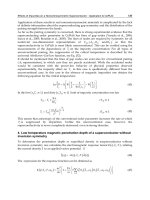
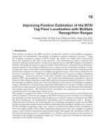
paper respectively. Simulations of the corresponding control inputs are shown in Fig. 3, in
which, the dash-dot line and the solid line represent respectively the input of the controller
of Lee, Park, and Chen (2001) and of the controller in the paper.

3.9 3.95 4
0
2000
4000
6000

Time (sec)
4 4.5 5 5.5
-100
0
100
200
300
400
500
Time
(
sec
)

Fig. 3. Control input of the two controllers (dash-dot line and solid line represent
respectively the result of Lee, Park, and Chen (2001) and the result of the paper)
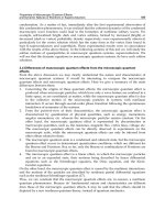
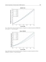
The simulated state trajectories and phase trajectory of the controlled Lorenz system are

shown respectively in Figs. 4 and 5, in which, all the uncertain parameters are generated
randomly within the allowable ranges.
Robust Control, Theory and Applications

388

Fig. 4. Ten-times simulated state trajectories of the controlled chaotic Lorenz system with
parametric uncertainties (all uncertain parameters are generated randomly within the
allowable ranges, and on the left- and right-hand sides are respectively the results of
controllers in Lee, Park, and Chen (2001) and in the paper)

0
10
20
30
40
50
-20
0
20
-20
0
20
40

x
3
(t)

x

1
(t)
end

x
2
(t)

Fig. 5. Ten-times simulated phase trajectories of the parametric uncertain Lorenz system
controlled by the presented method (all parameters are generated randomly within their
allowable ranges)
Robust Fuzzy Control of
Parametric Uncertain Nonlinear Systems Using Robust Reliability Method

389
It can be seen that the controller obtained by the presented method is effective, and the
control effect has no evident difference with that of the controller in Lee, Park, and Chen
(2001), but the control input of it is much lower. This shows that the presented method is
much less conservative.
Taking
3=
α
, which means that the allowable variation of all the uncertain parameters are
within 90% of their nominal values, by applying Theorem 3.3 and solving a corresponding
optimization problem of (64) with
3
*
=
α
, the gain matrices for deriving the fuzzy controller

obtained by the presented method become
[
]
[
]
12
-54.0211 32.5959 6.5886 , -50.0340 30.6071 10.4215
GG
=−− =−KK.
Obviously, the input of the controller in this case is also much lower than that of the
controller obtained by Lee, Park, and Chen (2001).
Secondly, when Theorem 3.4 is used, by solving two optimization problems corresponding
to (69) with
1
*
=
α
and
3
*
=
α
respectively, the gain matrices for deriving the controller are
found to be
[
]
[
]
[][]
*

12
*
12
20.8198 13.5543 3.2560 , 21.1621 13.1451 4.3928 ( 1).
-54.0517 32.6216 6.6078 , -50.0276 30.6484 10.4362 ( 3)
GG
GG
α
α
=−−− =−− =
=−− =− =
KK
KK

Note that the results based on Theorem 3.4 are in agreement, approximately, with those
based on Theorem 3.3.
5. Conclusion
In this chapter, stability of parametric uncertain nonlinear systems was studied from a new
point of view. A robust reliability procedure was presented to deal with bounded
parametric uncertainties involved in fuzzy control of nonlinear systems. In the method, the
T-S fuzzy model was adopted for fuzzy modeling of nonlinear systems, and the parallel-
distributed compensation (PDC) approach was used to control design. The stabilizing
controller design of uncertain nonlinear systems were carried out by solving a set of linear
matrix inequalities (LMIs) subjected to robust reliability for feasible solutions, or by solving
a robust reliability based optimization problem to obtain optimal controller. In the optimal
controller design, both the robustness with respect to uncertainties and control cost can be
taken into account simultaneously. Formulations used for analysis and synthesis are within
the framework of LMIs and thus can be carried out conveniently. It is demonstrated, via
numerical simulations of control of a simple mechanical system and of the chaotic Lorenz
system, that the presented method is much less conservative and is effective and feasible.

Moreover, the bounds of uncertain parameters are not required strictly in the presented
method. So, it is applicable for both the cases that the bounds of uncertain parameters are
known and unknown.
6. References
Ben-Haim, Y. (1996). Robust Reliability in the Mechanical Sciences, Berlin: Spring-Verlag
Breitung, K.; Casciati, F. & Faravelli, L. (1998). Reliability based stability analysis for actively
controlled structures.
Engineering Structures, Vol. 20, No. 3, 211–215
Robust Control, Theory and Applications

390
Chen, B.; Liu, X. & Tong, S. (2006). Delay-dependent stability analysis and control synthesis of
fuzzy dynamic systems with time delay.
Fuzzy Sets and Systems, Vol. 157, 2224–2240
Crespo, L. G. & Kenny, S. P. (2005). Reliability-based control design for uncertain systems.
Journal of Guidance, Control, and Dynamics, Vol. 28, No. 4, 649-658
Feng, G.; Cao, S. G.; Kees, N. W. & Chak, C. K. (1997). Design of fuzzy control systems with
guaranteed stability.
Fuzzy Sets and Systems, Vol. 85, 1–10
Guo, S. X. (2010). Robust reliability as a measure of stability of controlled dynamic systems
with bounded uncertain parameters.
Journal of Vibration and Control, Vol. 16, No. 9,
1351-1368
Guo, S. X. (2007). Robust reliability method for optimal guaranteed cost control of
parametric uncertain systems.
Proceedings of IEEE International Conference on Control
and Automation
, 2925-2928, Guangzhou, China
Hong, S. K. & Langari, R. (2000). An LMI-based H
∞

fuzzy control system design with TS
framework.
Information Sciences, Vol. 123, 163-179
Lam, H. K. & Leung, F. H. F. (2007). Fuzzy controller with stability and performance rules
for nonlinear systems.
Fuzzy Sets and Systems,Vol. 158, 147–163
Lee, H. J.; Park, J. B. & Chen, G. (2001). Robust fuzzy control of nonlinear systems with
parametric uncertainties.
IEEE Transactions on Fuzzy Systems, Vol. 9, 369–379
Park, J.; Kim, J. & Park, D. (2001). LMI-based design of stabilizing fuzzy controllers for
nonlinear systems described by Takagi-Sugeno fuzzy model.
Fuzzy Sets and
Systems
, Vol. 122, 73–82
Spencer, B. F.; Sain, M. K.; Kantor, J. C. & Montemagno, C. (1992). Probabilistic stability
measures for controlled structures subject to real parameter uncertainties.
Smart
Materials and Structures
, Vol. 1, 294–305
Spencer, B. F.; Sain, M. K.; Won C. H.; et al. (1994). Reliability-based measures of structural
control robustness.
Structural Safety, Vol. 15, No. 2, 111–129
Tanaka, K.; Ikeda, T. & Wang, H. O. (1996). Robust stabilization of a class of uncertain
nonlinear systems via fuzzy control: quadratic stabilizability, H
∞
control theory, and
linear matrix inequalities.
IEEE Transactions on Fuzzy Systems, Vol. 4, No. 1, 1–13
Tanaka, K. & Sugeno, M. (1992). Stability analysis and design of fuzzy control systems.
Fuzzy Sets and Systems, Vol. 45, 135–156

Teixeira, M. C. M. & Zak, S. H. (1999). Stabilizing controller design for uncertain nonlinear
systems using fuzzy models.
IEEE Transactions on Fuzzy Systems, Vol. 7, 133–142
Tuan, H. D. & Apkarian, P. (1999). Relaxation of parameterized LMIs with control
applications.
International Journal of Nonlinear Robust Control, Vol. 9, 59-84
Tuan, H. D.; Apkarian, P. & Narikiyo, T. (2001). Parameterized linear matrix inequality
techniques in fuzzy control system design.
IEEE Transactions on Fuzzy Systems, Vol.
9, 324–333
Venini, P. & Mariani, C. (1999). Reliability as a measure of active control effectiveness.
Computers and Structures, Vol. 73, 465-473
Wu, H. N. & Cai, K. Y. (2006). H
2
guaranteed cost fuzzy control design for discrete-time
nonlinear systems with parameter uncertainty.
Automatica, Vol. 42, 1183–1188
Xiu, Z. H. & Ren, G. (2005). Stability analysis and systematic design of Takagi-Sugeno fuzzy
control systems.
Fuzzy Sets and Systems, Vol. 151, 119–138
Yoneyama, J. (2006). Robust H
∞
control analysis and synthesis for Takagi-Sugeno general
uncertain fuzzy systems.
Fuzzy Sets and Systems, Vol. 157, 2205–2223
Yoneyama, J. (2007). Robust stability and stabilization for uncertain Takagi-Sugeno fuzzy
time-delay systems.
Fuzzy Sets and Systems, Vol. 158, 115–134

This chapter presents for SISO (Single Input Single Output) LTI (Linear Time Invariant)

systems, a detailed description of this robust control technique and two real experiences
where QFT has successfully applied at the University of Almería (Spain). It starts with
a QFT description from a theoretical point of view, afterwards section 3. 1 is devoted to
present two well-known software tools for QFT design, and after that two real applications
in agricultural spraying tasks and solar energy are presented. Finally, the chapter ends with
some conclusions.
2. Synthesis of SISO LTI uncertain feedback control systems using QFT
QFT is a methodology to design robust controllers based on frequency domain (Horowitz,
1993; Yaniv, 1999). This technique allows designing robust controllers which fulfil some
quantitative specifications. The Nichols plane is the key tool for this technique and is used to
achieve a robust design over the specified region of plant uncertainty. The aim is to design
a compensator C
(s) and a prefilter F(s ) (if it is necessary), as shown in Figure 1, so that
performance and stability specifications are achieved for the family of plants
℘( s) describing
aplantP
(s). Here, the notation
ˆ
a is used to represent the Laplace transform for a time domain
signal a
(t).
Fig. 1. Two degrees of freedom feedback system.
The QFT technique uses the information of the plant uncertainty in a quantitative way,
imposing robust tracking, robust stability, and robust attenuation specifications (among
others). The 2DoF compensator
{F, C}, from now onwards the s argument will be omitted
when necessary for clarity, must be designed in such a way that the plant behaviour variations
due to the uncertainties are inside of some specific tolerance margins in closed-loop. Here, the
family
℘( s) is represented by the following equation

℘( s)=

P
(s)=k
∏
n
i
=1
(s + z
i
)
∏
m
z
=1
(s
2
+ 2ξ
z
ω
0z
+ ω
2
0z
)
s
N
∏
a
r=1

(s + p
r
)
∏
b
t=1
(s
2
+ 2ξ
t
ω
0t
+ ω
2
0t
)
:(1)
k
∈ [k
min
, k
max
], z
i
∈ [z
i,min
, z
i,max
], p
r

∈ [p
r,min
, p
r,ma x
],
ξ
z
∈ [ξ
z,min
, ξ
z,max
], ω
0z
∈ [ω
0z ,min
, ω
0z ,max
],
ξ
t
∈ [ξ
t,min
, ξ
t,max
], ω
0t
∈ [ω
0t,min
, ω
0t,max

],
n
+ m < a + b + N

A typical QFT design involves the following steps:
392
Robust Control, Theory and Applications
1. Problem specification. The plant model with uncertainty is identified, and a set of
working frequencies is selected based on the system bandwidth, Ω
={ω
1
, ω
2
, ,ω
k
}.
The specifications (stability, tracking, input disturbances, output disturbances, noise, and
control effort) for each frequency are defined, and the nominal plant P
0
is selected.
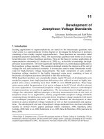
2. Templates. The quantitative information of the uncertainties is represented by a set of
points on the Nichols plane. This set of points is called template and it defines a graphical
representation of the uncertainty at each design frequency ω. An example is shown in
Figure 2, where templates of a second-order system given by P
(s)=k/s( s + a),with
k
∈ [1, 10] and a ∈ [1, 10] are displayed for the following set of frequencies Ω =
{
0.5, 1, 2, 4, 8, 15, 30, 60, 90, 120, 180} rad/s.
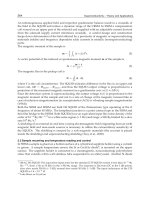
3. Bounds. The specifications settled at the first step are translated, for each frequency ω in

Ω set, into prohibited zones on the Nichols plane for the loop transfer function L
0
(jω)=
C(jω)P
0
(jω). These zones are defined by limits that are known as bounds.Thereexistso
many bounds for each frequency as specifications are considered. So, all these bounds for
each frequency are grouped showing an unique prohibited boundary.Figure3showsan
example for stability and tracking specifications.
Fig. 2. QFT Template example.
4. Loop shaping. This phase consists in designing the C controller in such a way that the
nominal loop transfer function L
0
(jω)=C(jω)P
0
(jω) fulfils the bounds calculated in the
previous phase. Figure 3 shows the design of L
0
where the bounds are fulfilled at each
design frequency.
5. Prefilter. The prefilter F is designed so that the closed-loop transfer function from reference
to output follows the robust tracking specifications, that is, the closed-loop system
variations must be inside of a desired tolerance range, as Figure 4 shows.
393
A Frequency Domain Quantitative Technique for Robust Control System Design
Fig. 3. QFT Bound and Loop Shaping example.
Fig. 4. QFT Prefilter example.
394
Robust Control, Theory and Applications
6. Validation. This step is devoted to verify that the closed-loop control system fulfils, for

the whole family of plants, and for all frequencies in the bandwith of the system, all the
specifications given in the first step. Otherwise, new frequencies are added to the set Ω,so
that the design is repeated until such specifications are reached.
The closed-loop specifications for system in Figure 1 are typically defined in time domain
and/or in the frequency domain. The time domain specifications define the desired outputs
for determined inputs, and the frequency domain specifications define in terms of frequency
the desired characteristics for the system output for those inputs.
In the following, these types of specifications are described and the specifications translation
problem from time domain to frequency domain is considered.
2.1 Time domain specifications
Typically, the closed-loop specifications for system in Figure 1 are defined in terms of the
system inputs and outputs. Both of them must be delimited, so that the system operates in a
predetermined region. For example:
1. In a regulation problem, the aim is to achieve a plant output close to zero (or nearby a
determined operation point). For this case, the time domain specifications could define
allowed operation regions as shown in Figures 5a and 5b , supposing that the aim is to
achieve a plant output close to zero.
2. In a reference tracking problem, the plant output must follow the reference input with
determined time domain characteristics. In Figure 5c a typical specified region is shown,
in which the system output must stay. The unit step response is a very common
characterization, due to it combines a fast signal (an infinite change in velocity at t
= 0
+
)
with a slow signal (it remains in a constant value after transitory).
The classical specifications such as rise time, settling time and maximum overshoot, are special
cases of examples in Figure 5. All these cases can be also defined in frequency domain.
2.2 Frequency domain specifications
The closed-loop specifications for system in Figure 1 are typically defined in terms of
inequalities on the closed-loop transfer functions for the system, as shown in Equations (2)-(7).

1. Disturbance rejection at the plant output:




ˆ
c
ˆ
d
o




=




1
1 + P(jω)C(jω)




≤ δ
po
(ω) ∀ω > 0, ∀P ∈ ℘ (2)
2. Disturbance rejection at the plant input:





ˆ
c
ˆ
d
i




=




P
(jω)
1 + P(jω)C(jω)




≤ δ
pi
(ω) ∀ω > 0, ∀P ∈ ℘ (3)
3. Stability:





ˆ
c
ˆ
rF




=




P
(jω) C(jω)
1 + P(jω)C(jω)




≤ λ ∀ω > 0, ∀P ∈ ℘ (4)
4. References Tracking:
B
l
(ω) ≤





ˆ
c
ˆ
r




=




F
(jω)P(jω)C(jω)
1 + P(jω)C(jω)




≤ B
u
(ω) ∀ω > 0, ∀P ∈ ℘ (5)
395
A Frequency Domain Quantitative Technique for Robust Control System Design
0 0.5 1 1.5 2 2.5 3 3.5 4 4.5 5
−1
−0.8
−0.6

−0.4
−0.2
0
0.2
0.4
0.6
0.8
1
time (s)
c
Allowed operation region
(a) Regulation problem
0 0.5 1 1.5 2 2.5 3 3.5 4 4.5 5
−1
−0.8
−0.6
−0.4
−0.2
0
0.2
0.4
0.6
0.8
1
time (s)
c
Allowed operation region
(b) Regulation problem for other initial conditions
0 0.5 1 1.5 2 2.5 3 3.5 4 4.5 5
0

0.2
0.4
0.6
0.8
1
time (s)
c
Allowed operation region
(c) Tracking problem
Fig. 5. Specifications examples in time domain.
396
Robust Control, Theory and Applications
5. Noise rejection:




ˆ
c
ˆ
n




=





P
(jω) C(jω)
1 + P(jω)C(jω)




≤ δ
n
(ω) ∀ω > 0, ∀P ∈ ℘ (6)
6. Control effort:




ˆ
u
ˆ
n




=




C
(jω)

1 + P(jω)C(jω)




≤ δ
ce
(ω) ∀ω > 0, ∀P ∈ ℘ (7)
For specifications in Eq. (2), (3) and (5), arbitrarily small specifications can be achieved
designing C so that
|C(jω)|→∞ (due to the appearance of the M-circle in the Nichols plot).
So, with an arbitrarily small deviation from the steady state, due to the disturbance, and with
a sensibility close to zero, the control system is more independent of the plant uncertainty.
Obviously, in order to achieve an increase in
|C(jω)| is necessary to increase the crossover
frequency
1
for the system. So, to achieve arbitrarily small specifications implies to increase
the bandwidth
2
of the system. Note that the control effort specification is defined, in this
context, from the sensor noise n to the control signal u. In order to define this specification
from the reference, only the closed-loop transfer function from the n signal to u signal must
be multiplied by F precompensator. However, in QFT, it is not defined in this form because of
F must be used with other purposes.
On the other hand, to increase the value of
|C(jω)| implies a problem in the case of the
control effort specification and in the case of the sensor noise rejection, since, as was previously
indicated, the bandwidth of the system is increased (so the sensor noise will affect the system
performance a lot). A compromise must be achieved among the different specifications.

The stability specification is related to the relative stability margins: phase and gain margins.
Hence, supposing that λ is the stability specification in Eq. (4), the phase margin is equal to
2
·arcsin(0.5λ) degrees, and the gain margin is equal to 20log
10
(1 + 1/λ) dB.
The output disturbance rejection specification limits the distance from the open-loop transfer
function L
(jω) to the point (− 1, 0) in Nyquist plane, and it sets an upper limit on the
amplification of the disturbances at the plan output. So, this type of specification is also
adequated for relative stability.
2.3 Translation of quantitative specifications from time to frequency domain
As was previously indicated, QFT is a frequency domain design technique, so, when the
specifications are given in the time domain (typically in terms of the unit step response), it
is necessary to translate them to frequency domain. One way to do it is to assume a model for
the transfer function T
cr
, closed-loop transfer function from reference r to the output c,andto
find values for its parameters so that the defined time domain limits over the system output
are satisfied.
2.3.1 A first-order model
Lets consider the simplest case, a first-order model given by T
cr
(s)=K/(s + a), so that when
r
(t) is an unit step the system output is given by c(t)=(K/a)(1 −e
−at
). Then, in order to
reach c
(t)=r(t) for a time t large enough, K should be K = a.

1
The crossover frequency for a system is defined as the frequency in rad/s such that the magnitude of
the open-loop transfer function L
(jω)=P(jω)C(jω) is equal to zero decibels (dB).
2
The bandwith of a system is defined as the value of the frequency ω
b
in rad/s such that
|T
cr
(jω
b
)/T
cr
(0)|
dB
= -3 dB, where T
cr
is the closed-loop transfer function from the reference r to the
output c.
397
A Frequency Domain Quantitative Technique for Robust Control System Design
For a first-order model τ
c
= 1/a = 1/ω
b
is the time constant (represents the time it takes the
system step response to reach 63.2% of its final value). In general, the greater the bandwith is,
the faster the system output will be.
One important difficulty for a first-order model considered is that the first derivative for the

output (in time infinitesimaly after zero, t
= 0
+
)isc = K, when it would be desirable to be 0.
So, problems appear at the neighborhood of time t
= 0. In Figure 6 typical specified time limits
(from Eq. (5) B
l
and B
u
are the magnitudes of the frequency response for these time domain
limits) and the system output are shown when a first-order model is used. As observed,
problems appear at the neighborhood of time t
= 0. On the other hand the first-order model
does not allow any overshoot, so from the specified time limits the first order model would
be very conservative. Hence, a more complex model must be used for the closed-loop transfer
function T
cr
.
0 1 2 3 4 5 6 7 8 9 10
0
0.2
0.4
0.6
0.8
1
1.2
1.4
1.6
time (s)

Limits
c=2
Fig. 6. Inadequate first-order model.
2.3.2 A second-order model
In this case, two free parameters are available (assuming unit static gain): the damping factor
ξ and the natural frequency ω
n
(rad/s). The model is given by
T
(s)=
ω
2
n
s
2
+ 2ξω
n
s + ω
2
n
(8)
The unit step response, depending on the value of ξ,isgivenby
398
Robust Control, Theory and Applications
c(t)=
⎧
⎪
⎪
⎨
⎪

⎪
⎩
1
−e
−ξω
n
t
(cos(ω
n

1 −ξ
2
t )+
ξω
n
ω
n
√
1−ξ
2
sin(ω
n

1 −ξ
2
t )) if ξ < 1
1
−e
−ξω
n

t
(cosh(ω
n

ξ
2
−1t)+
ξω
n
ω
n
√
ξ
2
−1
sinh( ω
n

1 −ξ
2
t )) if ξ > 1
1
−e
−ξω
n
t
(1 + ω
n
t ) if ξ = 1
In practice, the step response for a system usually has more terms, but normally it contains

a dominant second-order component with ξ
< 1. The second-order model is very popular in
control system design in spite of its simplicity, because of it is applicable to a large number of
systems. The most important time domain indexes for a second-order model are: overshoot,
settling time, rise time, damping factor and natural frequency. In frequency domain, its most
important indexes are: resonance peak (related with the damping factor and the overshoot),
resonance frequency (related with the natural frequency), and the bandwidth (related with
the rise time). The resonance peak is defined as
max
ω
|T
cr
(jω) |

M
p
. The resonance frequency
ω
p
is defined as the frequency at which |T
cr
(jω
p
)| = M
p
. One way to control the overshoot
is setting an upper limit over M
p
. For example, if this limit is fixed on 3 dB, and the practical
T

cr
(jω) for ω in the frequency range of interest is ruled by a pair of complex conjugated poles,
then this constrain assures an overshoot lower than 27%.
In (Horowitz, 1993) tables with these relations are proposed, where, based on the experience of
Professor Horowitz, makes to set a second-order model to be located inside the allowed zone
defined by the possible specifications. As Horowitz suggested in his book, if the magnitude of
the closed-loop transfer function T
cr
is located between frequency domain limits B
u
(ω) and
B
l
(ω) in Eq. (5), then the time domain response is located between the corresponding time
domain specifications, or at most it would be satisfied them in a very approximated way.
2.3.3 A third-order model with a zero
A third-order model with a unit static gain is given by
T
(s)=
μω
3
n
(s
2
+ 2ξω
n
s + ω
2
n
)(s + μω

n
)
(9)
For values of μ less than 5, a similar behaviour as if the pole is not added to the second-order
model is obtained . So, the model in Eq. (8) would must be used.
If a zero is added to Eq. (9), it results
T
(s)=
(
1 + s/λξω
n
)μω
3
n
(s
2
+ 2ξω
n
s + ω
2
n
)(s + μω
n
)
(10)
The unit responses obtained in this case are shown in Figure 7 for different values of λ.
As shown in Figure 7, this model implies an improvement with respect to that in Eq. (8),
because of it is possible to reduce the rise time without increasing the overshoot. Obviously, if
ω
n

> 1, then the response is ω
n
times faster than the case with ω
n
= 1(slowerforω
n
< 1). In
(Horowitz, 1993), several tables are proposed relating parameters in Eq. (10) with time domain
parameters as overshoot, rise time and settling time.
399
A Frequency Domain Quantitative Technique for Robust Control System Design
0 1 2 3 4 5 6 7 8 9 10
0
0.2
0.4
0.6
0.8
1
1.2
1.4
1.6
ω
n
·time
λ=1
λ=0.3
λ=0.5
λ=0.7
Fig. 7. Third-order model with a zero for μ = 5andξ = 1.
There exist other techniques to translate specifications from time domain to frequency

domain, such as model-based techniques, where based on the structures of the plant and
the controller, a set of allowed responses is defined. Another technique is that presented in
(Krishnan and Cruickshanks, 1977), where the time domain specifications are formulated as

t
0
|c(τ) − m(τ)|
2
dτ ≤

t
0
v
2
(τ)dτ,withm(t) and v(t) specified time domain functions, and
where it is established that the energy of the signal, difference between the system output and
the specification m
(t), must be enclosed by the energy of the signal v(t), for each instant t,and
with a translation to the frequency domain given by the inequality
|
ˆ
c
(jω) −
ˆ
m
(jω) |≤|
ˆ
v
(jω) |.
In (Pritchard and Wigdorowitz, 1996) and (Pritchard and Wigdorowitz, 1997), the relation

time-frequency is studied when uncertainty is included in the system, so that it is possible
to know the time domain limits for the system response from frequency response of a set
of closed-loop transfer functions from reference to the output. This technique may be used
to solve the time-frequency translation problem. However, the results obtained in translation
from frequency to time and from time to frequency are very conservative.
2.4 Controller design
Now, the procedure previously introduced is explained more in detail. The aim is to design
the 2DoF controller
{F, G} in Figure 1, so that a subset of specifications introduced in section
2.2is satisfied, and the stability of the closed-loop system for all plant P in
℘ is assured.
The specifications in section 2. 2are translated in circles on Nyquist plane defining allowed
zones for the function L
(jω)=P(jω)C(jω). The allowed zone is the outside of the circle for
specifications in Eq. (2)-(6), and the inside one for the specification in Eq. (7). Combining the
allowed zones for each function L corresponding to each plant P in
℘, a set of restrictions for
controller C for each frequency ω is obtained. The limits of these zones represented in Nichols
400
Robust Control, Theory and Applications
plane are called bounds or boundaries. These constrains in frequency domain can be formulated
over controller C or over function L
0
= P
0
C,foranyplantP
0
in ℘ (so-called nominal plant).
In order to explain the detailed design process, the following example, from (Horowitz, 1993),
is used. Lets suppose the plant in Figure 1 given by

℘ =

P
(s)=
k
s(s + a)
with k ∈ [1, 20] and a ∈ [1,5]

(11)
corresponding to a range of motors and loads, where the equation modeling the motor
dynamic is J
¨
c
+ B
˙
c = Ku,withk = K/J and a = B/J in Eq. (11). Lets suppose the tracking
specifications given by
B
l
(ω) ≤|T
cr
(jω) |
dB
=




F
(jω)P(jω)C(jω)

1 + P(jω)C(jω)




dB
≤ B
u
(ω) ∀P ∈ ℘ ∀ω > 0 (12)
showninFigure8.InFigure9,thedifferenceδ
(ω)=B
u
(ω) − B
l
(ω) is shown for each
frequency ω. It is easy to see that in order to satisfy the specifications in Eq. (12), the following
inequality must be satisfied
Δ
|T
cr
(jω) |
dB
= max
P∈℘




P
(jω) C(jω)

1 + P(jω)C(jω)




dB
−min
P∈℘




P
(jω) C(jω)
1 + P(jω)C(jω)




dB
≤
≤
δ(ω)=B
u
(ω) − B
l
(ω) ∀P ∈ ℘ ∀ω > 0
(13)
10
−1

10
0
10
1
10
2
−100
−80
−60
−40
−20
0
20
Frequency (rad/s)
|·| − dB
Original
B
u
(ω)
B
l
(ω)
B
u
(ω) enlarged
B
l
(ω) enlarged
Fig. 8. Tracking specifications (variations over a nominal).
401

A Frequency Domain Quantitative Technique for Robust Control System Design
10
−1
10
0
10
1
10
2
0
10
20
30
40
50
60
Frequency (rad/s)
Dif. − dB
Original
Enlarged
Fig. 9. Specifications on the magnitude variations for the tracking problem.
Making L
= PC large enough, for each plant P in ℘, and for a frequency ω, it is possible
to achieve an arbitrarily small specification δ
(ω).However,thisisnotpossibleinpractice,
since the system bandwidth must be limited in order to minimize the influence of the sensor
noise at the plant input. When C has been designed to satisfy the specifications in Eq. (13), the
second degree of freedom, F, is used to locate those variations inside magnitude limits B
l
(ω)

and B
u
(ω).
In order to design the first degree of freedom, C, it is necessary to define a set of constrains on
C or on L
0
in the frequency domain, what guarantee that if C (respectively L
0
) satisfies those
restrictions then the specifications are satisfied too. As commented above, these constrains are
called bounds or boundaries in QFT, and in order to compute them it is necessary to take into
account:
(i) A set of specifications in frequency domain, that in the case of tracking problem, are given
by Eq. (13), and that in other cases (disturbance rejection, control effort, sensor noise, ) are
similar as shown in section 2.2.
(ii) An object (representation) modeling the plant uncertainty in frequency domain, so-called
template.
The following sections explain more in detail the meaning of the templates and the bounds.
Computation of basic graphical elements to deal with uncertainties: templates
If there is no uncertainty in plant, the set ℘ would contain only one transfer function, P,and
for a frequency, ω, P
(jω) would be a point in the Nichols plane. Due to the uncertainty, a set
of points, for each frequency, appears in the Nichols plane. One point for each plant P in
℘.
These sets are called templates. For example, Figure 10 shows the template for ω
= 2rad/s,
corresponding to the set:
402
Robust Control, Theory and Applications
−155 −150 −145 −140 −135 −130 −125 −120 −115 −110

−25
−20
−15
−10
−5
0
5
10
15
Angle(P) − degrees
|P| − dB
k=20
k=1
k=2
a=1
a=2
a=3
A
B
C
D
E
F
Fig. 10. Template for frequency ω = 2 rad/s and the plant given by Eq. (11).
(ω = 2)=

k
2j(2j + a)
: k ∈ [1, 20] and a ∈ [1, 5]


.
For k
= 1 and driving a from 1 to 5, the segment ABC is obtained in Figure 10. For a = 3and
driving k from 1 to 20, the segment BE is calculated. For k
= 20 and driving a from 1 to 5, the
segment DEF is obtained.
Choosing a plant P
0
belonging to the set ℘, the nominal open-loop transfer function is defined
as L
0
= P
0
C.Inordertoshiftatemplate in the Nichols plane, a quantity must be added in
phase (degrees) and other quantity in magnitude (decibels) to all points. Using the nominal
point P
0
(jω) as representative of the full template at frequency ω and shaping the value of the
nominal L
0
(jω)=P
0
(jω) C(jω) using C(jω),itisequivalenttoadd|C(jω)|
dB
in magnitude
and An gle
(C(jω)) degrees in phase to each point P(jω) (with magnitude in decibels and
phase in degrees) inside the template at frequency ω. So, the shaping of the nominal open-loop
transfer function at frequency ω (using the degree of freedom C ), is equivalent to shift the
template at that frequency ω to a specific location in the Nichols plane.

The choice of the nominal plant for a template is totally free. The design method is valid
independently of this choice. However, there exist rules for the more adequate choice in
specific situations (Horowitz, 1993).
As was previously indicated, there exists a template for each frequency, so that after the
definition of the specifications for the control problem, the following step is to define a set
of design frequencies Ω. Then, the templates would be computed for each frequency ω in Ω.
Once the specifications have been defined and the templates have been computed, the third
step is the computation of boundaries using these graphical objects and the specifications.
403
A Frequency Domain Quantitative Technique for Robust Control System Design
Derivation of boundaries from templates and specifications
Now, zones on Nichols plane are defined for each frequency ω in Ω, so that if the nominal of
the template shifted by C
(jω) is located inside that zone, then the specifications are satisfied.
For each specification in section 2. 2and for each frequency ω in Ω,usingthetemplate and
the corresponding specification, the boundary must be computed. Details about the different
types of bounds and the most important algorithms to compute them can be found in (Moreno
et al., 2006). In general, a boundary at frequency ω defines a limit of a zone on Nichols plane
so that if the nominal L
0
(jω) of the shifted template is located inside that zone, then some
specifications are satisfied. So, the most single appearance of a boundary defines a threshold
value in magnitude for each phase φ in the Nichols plane, so that if An gl e
(L
0
(jω)) = φ,then
|L
0
(jω) |
dB

must be located above (or below depending on the type of specification used to
compute the boundary) that threshold value.
It is important to note that sometimes redefinition of the specifications is necessary. For
example, for system in Eq. (11), for ω
≥ 10 rad/s the templates have similar dimensions, and
the specifications from Eq. (13) in Figure 9 are identical. Then, the boundaries for ω
≥ 10 rad/s
will be almost identical. The function L
0
(jω) must be above the boundaries for all frequencies,
including ω
≥ 10 rad/s, but this is unviable due to it must be satisfied that L
0
(jω) → 0
when ω
→ ∞. Therefore, it is necessary to open the tracking specifications for high frequency
(where furthermore the uncertainty is greater), such as it is shown in Figure 8. On the other
hand, it must be also taken into account that for a large enough frequency ω, the specification
δ
(ω) in Eq. (13) must be greater or equal than
max
P∈℘
|P(jω)|
dB
−
min
P∈℘
|P(jω)|
dB
such that, for

a small value of L
0
(jω) for these frequencies, the specifications are also satisfied. The effect
of this enlargement for the specifcations is negligible when the modifications are introduced
at a frequency large enough. These effects are notable in the response at the neighborhood of
t
= 0.
Considering the tracking bounds as negligible from a specific frequency (in the sense that
the specification is large enough), it implies that the stability boundaries are the dominant
ones at these frequencies. As was mentioned above, since the templates are almost identical at
high frequencies and the stability specification λ is independent of the frequency, the stability
bounds are also identical and only one of them can be used as representative of the rest. In
QFT, this boundary is usually called high frequency bound, and it is denoted by B
h
.
Notice that the use of a discrete set of design frequencies Ω does not imply any problem.
The variation of the specifications and the variation of the appearance of the templates from a
frequency ω
−
to a frequency ω
+
,withω
−
< ω < ω
+
, is smooth. Anyway, the methodology
let us discern the specific cases in which the number of elements of Ω is insufficient, and let
us iterate in the design process to incorporate the boundaries for those new frequencies, then
reshaping again the compensator
{F, C}.

Design of the nominal open-loop transfer function fulfilling the boundaries
In this stage, the function L
0
(jω) must be shaped fulfilling all the boundaries for each frequency.
Furthermore, It must assure that the transfer function 1
+ L(s) has no zeros in the right half
plane for any plant P in
℘. So, initially L
0
= P
0
(C = 1) and poles and zeros are added to this
function (poles and zeros of the controller C) in order to satisfy all of these restrictions on the
Nichols plane. In this stage, only using the function L
0
, it is possible to assure the fulfillment of
the specifications for all of the elements in the set
℘ when L
0
(jω) is located inside the allowed
zones defined by the boundary at frequency ω (computed from the corresponding template at
that frequency, and from the specifications).
404
Robust Control, Theory and Applications
Obviously, there exists an infinite number of acceptable functions L
0
satisfying the boundaries
and the stability condition. In order to choose among all of these functions, an important factor
to be considered is the sensor noise effect at the plant input. The closed-loop transfer function
from noise n to the plant input u is given by

T
un
(s)=
−
C(s)
1 + P(s)C(s)
=
−
L(s)/P(s)
1 + L(s)
.
In the range of frequencies in which
|L(jω)| is large (generally low frequency), |T
un
(jω) |→
|
1/P(jω)|, so that the value of |T
un
(jω) | at low frequency is independent on the design
chosen for L. In the range of frequencies where
|L(jω)| is small (generally high frequency),
|T
un
(jω) |→|G(jω)|. These two asymptotes cross between themselves at the crossover
frequency.
In order to reduce the influence of the sensor noise at the plant input,
|C(jω)|→0when
ω
→ ∞ must be guaranteed. It is equivalent to say that |L
0

(jω) | must be reduced as fast
as possible at high frequency. A conditionally stable
3
design for L
0
is especially adequate to
achieve this objective. However, as it is shown in (Moreno et al., 2010) this type of designs
supposes a problem when there exists a saturation non-linearity type in the system.
Design of the prefilter
At this point, only the second degree of freedom, F,mustbeshaped.ThecontrollerC,
designed in the previous step, only guarantees that the specifications in Eq. (13) are satisfied,
but not the specifications in Eq. (12). Using F, it is possible to guarantee that the specifications
in Eq. (12) are satisfied when with C the specifications in Eq. (13) are assured.
In order to design F , the most common method consists of computing for each frequency ω
the following limits
F
u
(ω)=




max
P∈℘




P
(jω) C(jω)

1 + P(jω)C(jω)




dB
−B
u
(ω)




and
F
l
(ω)=




min
P∈℘




P
(jω) C(jω)
1 + P(jω)C(jω)





dB
− B
l
(ω)




and shaping F adding poles and zeros until F
l
(ω) ≤|F(jω)|≤F
u
(ω) for all frequency ω in
Ω.
Validation of the design
This is the last step in the design process and consists in studying the magnitude of the
different closed-loop transfer functions, checking if the specifications for frequencies outside
of the set Ω are satisfied. If any specification is not satisfied for a specific frequency, ω
p
,
then this frequency is added to the set Ω, and the corresponding template and boundary are
3
A system is conditionally stable if a gain reduction of the open-loop transfer function L drives the
closed-loop poles to the right half plane.
405
A Frequency Domain Quantitative Technique for Robust Control System Design

computed for that frequency ω
p
. Then, the function L
0
is reshaped, so that the new restriction
is satisfied. Afterwards, the precompensator F is reshaped, and finally the new design is
validated. So, an iterative procedure is followed until the validation result is satisfactory.
3. Computer-based tools for QFT
As it has been described in the previous section, the QFT framework evolves several
stages, where a continuous re-design process must be followed. Furthermore, there are some
steps requiring the use of algorithms to calculate the corresponding parameters. Therefore,
computer-based tools as support for the QFT methodology are highly valuable to help in
the design procedure. This section briefly describes the most well-known tools available in
the literature, The Matlab QFT Toolbox (Borghesani et al., 2003) and SISO-QFTIT (Díaz et al.,
2005a),(Díaz et al., 2005b).
3.1 Matlab QFT toolbox
The QFT Frequency Domain Control Design Toolbox is a commercial collection of Matlab
functions for designing robust feedback systems using QFT, supported by the company
Terasoft, Inc (Borghesani et al., 2003). The QFT Toolbox includes a convenient GUI that
facilitates classical loop shaping of controllers to meet design requirements in the face of
plant uncertainty and disturbances. The interactive GUI for shaping controllers provides
a point-click interface for loop shaping using classical frequency domain concepts. The
toolbox also includes powerful bound computation routines which help in the conversion of
closed-loop specifications into boundaries on the open-loop transfer function (Borghesani et al.,
2003).
The toolbox is used as a combination of Matlab functions and graphical interfaces to perform
a complete QFT design. The best way to do that is to create a Matlab script including all the
required calls to the corresponding functions. The following lines briefly describe the main
steps and functions to use, where an example presented in (Borghesani et al., 2003) is followed
for a better understanding (a more detailed description can be found in (Borghesani et al.,

2003)).
The example to follow is described by:
℘ =

P
(s)=
k
(s + a)(s + b)
: k =[1, 2, 5, 8, 10], a =[1, 3, 5], b =[20, 25, 30]

. (14)
Once the process and the associated uncertainties are defined, the different steps, explained
in section 2., to design the robust control scheme using the QFT toolbox are described in the
following:
• Template computation. First, the transfer function models representing the process
uncertainty must be written. The following code calculates a matrix of 40 plant elements
which is stored in the variable P and represents the system defined by Eq. (14).
» c = 1; k = 10; b = 20;
» for a = linspace(1,5,10),
» P(1,1,c) = tf(k,[1,a+b,a*b]); c = c + 1;
»end
» k = 1; b = 30;
» for a = linspace(1,5,10),
406
Robust Control, Theory and Applications
» P(1,1,c) = tf(k,[1,a+b,a*b]); c = c + 1;
»end
» b = 30; a = 5;
» for k = linspace(1,10,10),
» P(1,1,c) = tf(k, [1,a+b,a*b]); c = c + 1;

»end
» b = 20; a = 1;
» for k = linspace(1,10,10),
» P(1,1,c) = tf(k, [1,a+b,a*b]); c = c + 1;
»end
Then, the nominal element is selected:
» nompt=21;
and the frequency array is set:
» w = [0.1, 5, 10, 100];
Finally, the templates are calculated and visualized using the pl o tt mpl function (see
(Borghesani et al., 2003) for a detailed explanation):
» plottmpl(w,P,nompt);
obtaining the templates shown in Figure 11.
Fig. 11. Matlab QFT Toolbox. Templates for example in Eq. (14)
• Specifications. In this step, the system specifications must be defined according to Eq. (2)-(7).
Once the specifications are determined, the corresponding bounds on the Nichols plane are
computed. The following source code shows the use of specifications in Eq. (2)-(4) for this
example.
A stability specification of λ
= 1.2 in Eq. (4) corresponding to a gain margin (GM) ≥ 5.3
dB and a phase margin (PM)
= 49.25 degrees is given:
» Ws1 = 1.2;
Then, the stability bounds are computed using the function siso b nds (see (Borghesani et al.,
2003) for a detailed explanation) and its value is stored in the variable bdb1:
407
A Frequency Domain Quantitative Technique for Robust Control System Design
» bdb1 = sisobnds(1,w,Ws1,P,0,nompt);
Lets now consider the specifications for output and input disturbance rejection cases, from
Eq. (2)-(3). For the case of the output disturbance specification, the performance weight for

the bandwidth [0,10] is defined as
» Ws2 = tf(0.02*[1,64,748,2400],[1,14.4,169]);
and the bounds are computed in the following way
» bdb2 = sisobnds(2,w(1:3),Ws2,P,0,nompt);
For the input disturbance case, the specification is defined as constant for
» Ws3 = 0.01;
calculating the bounds as
» bdb3 = sisobnds(3,w(1:3),Ws3,P,0,nompt);
also for the bandwidth [0,10].
Once the specifications are defined and the corresponding bounds are calculated. For each
frequency they can be combined using the following functions:
» bdb = grpbnds(bdb1,bdb2,bdb3); // Making a global structure
» ubdb = sectbnds(bdb); // Combining bounds
The resulting bounds which will be used for the loop-shaping stage are shown in Figure 12.
This figure is obtained using the plo tbn ds function:
»plotbnds(ubdb);
Fig. 12. Matlab QFT Toolbox. Boundaries for example (14)
• Loop-shaping. After obtaining the stability and performance bounds, the next step consists in
designing (loop shaping) the controller. The QFT toolbox includes a graphical interactive
GUI, lpshape, which helps to perform this task in an straightforward way. Before using
this function, it is necessary to define the frequency array for loop shaping, the nominal
plant, and the initial controller transfer function. Therefore, these variables must be set
previously, where for this example are given by:
» wl = logspace(-2,3,100); // frequency array for loop shaping
» C0 = tf(1,1); // Initial Controller
408
Robust Control, Theory and Applications
» L0=P(1,1,nompt)*C0; // Nominal open-loop transfer function
Having defined these variables, the graphical interface is opened using the following line:
» lpshape(wl,ubdb,L0,C0);

obtaining the window shown in Figure 13. As shown from this figure, the GUI allows to
modify the control transfer functions adding, modifying, and removing poles and zeros.
This task can be done from the options available at the right area of the windows or
dragging interactively on the loop L
0
(s)=P
0
(s)C(s) represented by the black line on
the Nichols plane.
For this example, the final controller is given by (Borghesani et al., 2003)
C
(s)=
379(
s
42
+ 1)
s
2
247
2
+
s
247
+ 1
(15)
Fig. 13. Matlab QFT Toolbox. Loop shaping for example in Eq. (14)
• Pre-filter design. When the control design requires tracking of reference signals, although
this is not the case for this example, a pre-filter F
(s) must be used in addition to
the controller C

(s) such as discussed in section 2 The prefilter can be also designed
interactively using a graphical interface similar to that described for the loop shaping stage.
To run this option, the pfshapefunction must be used (see (Borghesani et al., 2003) for more
details).
• Validation. The control system validation can be done testing the resulting robust controller
for all uncertain plants defined by Eq. (14) and checking that the different specifications
are fulfilled for all of them. This task can be performed directly programming in Matlab or
using the chksiso function from the QFT toolbox.
3.2 An interactive tool based in Sysquake: SISO-QFTIT
SISO-QFTIT is a free software interactive tool for robust control design using the QFT
methodology (Díaz et al., 2005a;b). The main advantages of SISO-QFTIT compared to other
existing tools are its easiness of use and its interactive nature. In the tool described in the
previous section, a combination between code and graphical interfaces must be used, where
409
A Frequency Domain Quantitative Technique for Robust Control System Design
some interactive features are also provided for the loop shaping and filter design stages.
However, with SISO-QFTIT all the stages are available from an interactive point of view.
As commented above, the tool has been implemented in Sysquake, a Matlab-like language
with fast execution and excellent facilities for interactive graphics (Piguet, 2004). Windows,
Mac, and Linux operating systems are supported. Since this tool is completely interactive, one
consideration that must be kept in mind is that the tool’s main feature -interactivity- cannot
be easily illustrated in a written text. Thus, the reader is cordially invited to experience the
interactive features of the tool.
The users mainly should operate with only mouse operations on different elements in the
window of the application or text insertion in dialog boxes. The actions that they carry out are
reflected instantly in all the graphics in the screen. In this way the users take aware visually
of the effects that produce their actions on the design that they are carrying out. This tool is
specially conceived as much as for beginner users that want to learn the QFT methodology, as
for expert users (Díaz et al., 2005b).
The user can work with SISO-QFTIT in two different but not excluding ways (Díaz et al.,

2005b):
• Interactive mode. In this work form, the user selects an element in the window and drags
it to take it to a certain value, their actions on this element are reflected simultaneously on
all the present figures in the window of the tool.
• Dialogue mode. In this work form, the user should simply go selecting entrances of the
Settings menu and correctly fill the blanks of dialog boxes.
Such as commented in the manual of this interactive software tool, its main interactive
advantages and options are the following (Díaz et al., 2005b):
• Variations that take place in the templates when modifying the uncertainty of the different
elements of the plant or in the value of the template calculation frequency.
• Individual or combined variation on the bounds as a result of the configuration of
specifications, i.e., by adding zeros and poles to the different specifications.
• The movement of the controller zeros and poles over the complex plane and the
modification of its symbolic transfer function when the open loop transfer function is
modified in the Nichols plane.
• The change of shape of the open loop transfer function in the Nichols plane and the
variation of the expression of the controller transfer function when any movement,
addition or suppression of its zeros or poles in the complex plane.
• The changes that take place in the time domain representation of the manipulated and
controlled variables due to the modification of the nominal values of the different elements
of the plant.
• The changes that take place in the time domain representation of the manipulated and
controlled variables due to the introduction of a step perturbation at the input of the plant.
The magnitude and the occurrence instant of the perturbation is configured by the user by
means of the mouse.
Such as pointed out above, the interactive capabilities of the tool cannot be shown in a
written text. However, some screenshots for the example used with the Matlab QFT toolbox
are provided. Figure 14a shows the resulting templates for the process defined by Eq. (14).
410
Robust Control, Theory and Applications

Notice that with this tool, the frequencies, the process uncertainties and the nominal plant
can be interactively modified. The stability bounds are shown in Figure 14b. The radiobuttons
available at the top-right side of the tool allow to choose the desired specification. Once the
specification is selected, the rest of the screen is changed to include the specification values
in an interactive way. Figure 15a displays the loop shaping stage with the combination of
the different bounds (same result than in Figure 13). The figure also shows the resulting loop
shaping for controller (15). Then, the validation screen is shown in Figure 15b, where it is
possible to check interactively if the robust control design satisfies the specifications for all
uncertain cases. Although for this example it is not necessary to design the pre-filter for the
tracking specifications, this tool also provides a screen where it is possible to perform this task
(see an example in Figure 16).
(a) QFT Templates (b) Stability bounds
Fig. 14. SISO-QFTIT. Templates and bounds for the example described in Eq. (14)
(a) Loop shaping (b) Validation
Fig. 15. SISO-QFTIT. Loop shaping and validation for the example described in Eq. (14)
4. Practical applications
This section presents two industrial projects where the QFT technique has been successfully
used. The first one is focused on the pressure control of a mobile robot which was design
411
A Frequency Domain Quantitative Technique for Robust Control System Design